Fault-Tolerant Time-Varying Formation Trajectory Tracking Control for Multi-Agent Systems with Time Delays and Semi-Markov Switching Topologies

Abstract

The fault-tolerant time-varying formation (TVF) trajectory tracking control problem is investigated in this paper for uncertain multi-agent systems (MASs) with external disturbances subject to time delays under semi-Markov switching topologies. Firstly, based on the characteristics of actuator faults, a failure distribution model is established, which can better describe the occurrence of the failures in practice. Secondly, switching the network topologies is assumed to follow a semi-Markov stochastic process that depends on the sojourn time. Subsequently, a novel distributed state-feedback control protocol with time-varying delays is proposed to ensure that the MASs can maintain a desired formation configuration. To reduce the impact of disturbances imposed on the system, the $H_{\infty }$ performance index is introduced to enhance the robustness of the controller. Furthermore, by constructing an advanced Lyapunov–Krasovskii (LK) functional and utilizing the reciprocally convex combination theory, the TVF control problem can be transformed into an asymptotic stability issue, achieving the purpose of decoupling and reducing conservatism. Furthermore, sufficient conditions for system stability are obtained through linear matrix inequalities (LMIs). Eventually, the availability and superiority of the theoretical results are validated by three simulation examples.

1. Introduction

With the expeditious development of computational science and artificial intelligence, multi-agent system (MAS) cooperative control has achieved significant advancements in the fields of physics and engineering over the past few decades, encompassing consensus control [1], containment control [2], formation control [3], and flocking [4]. As an important branch of cooperative control, formation control aims to enable a group of agents capable of information interaction to form the required formation configuration according to task requirements. Compared with the three classical methods of leader–follower [5], virtual structure [6], and behavior-based [7], the consensus-based [8] formation control approach designs a distributed controller to achieve consensus in certain variables through the network information interaction between each agent and its neighbors, which has stronger robustness and better scalability.

As a result, inspired by the consensus theory, consensus-based formation control has become a research hotspot in the field of MAS cooperative control in recent years, and fruitful achievements have been achieved in this field. In the face of communication delays, Kang et al. [9] addressed the TVF control problem of unmanned aerial vehicle swarm systems (UAVSSs) by constructing an advanced LK functional for stability analysis. To suppress the influence of external disturbances on the system, Shahbazi et al. [10] realized the formation control of spacecraft via robust control theory. Cheng et al. [11] proposed a distributed $H_{\infty }$ controller with communication delays for MASs to realize the expected TVF trajectory tracking under the condition of delays and disturbances occurring simultaneously. In [12], the authors carried out the TVF problem of nonlinear MASs with uncertain parameters through the neural network-based adaptive feedback control. Unfortunately, only one or two problems were considered in the above studies. However, it never rains but it pours, because with communication bandwidth constraints and changeable environments, time-varying communication delays (TVCDs), external disturbances, and uncertainties of MASs are often tightly coupled at the same time, which results in a great challenge to the realization of TVF. Thus, the dilemma caused by the simultaneous coupling of these three problems is our first starting point.

In practice, the communication topology usually varies with environment alteration. For instance, when multiple autonomous underwater vehicles (AUVs) perform reconnaissance missions, the communication between them may be disrupted due to external disturbance or large transmission delay, necessitating the re-establishment of connections and a switch in the MAS’ communication topology. Therefore, the system parameters may change and the topology structure may switch randomly with time in the harsh and complex space environment. Since the Markovian process has the ability of describing the random variation in communication conditions, MASs that submit to Markovian switching topologies (MSTs) have attracted the attention of researchers in recent years [13,14,15]. Additionally, the MST methods provide state transition modeling, robustness, and adaptability. Nevertheless, it is worth noting that for Markovian switching topologies, the sojourn time on each topology obeys exponential distribution, and transition rates between the two topologies remain constant. This fixed switching rate restricts the application scope such that it may impair the robustness of MASs, resulting in failure to respond quickly to environmental changes. To eliminate this dilemma, researchers have explored the semi-Markov process in order to accommodate different distributions for sojourn time and permit time-varying switching rates. Consequently, the semi-Markov switching topologies (SMSTs) approach provides a more flexible communication connection strategy, which enables MASs to better adapt to complex environment and variable task requirements. Yet, a wealth of research has solved the issues of SMSTs analysis and synthesis, including stability investigation [16], event-triggered consensus [17], containment control [18], $H_{\infty }$ leader-following consensus [19], and neural networks [20]. Despite these advancements, the study of SMSTs used in the field of TVF trajectory tracking control has received poor attention. The study of this problem becomes our second starting point.

It is widely acknowledged that faults within MASs are ineluctable, potentially deteriorating the performance of systems and consequently causing systems to crash. Roughly speaking, sensor faults, actuator faults, and communication faults are the main sources of MAS faults [21]. To solve this thorny challenge, fault-tolerant control (FTC) methods are an effective way to address the failure problems. The purpose of FTC is to maintain the system’s stability and robust admissible performance when the system encounters faults. Since it was first proposed in [22], it has flourished into various FTC methods, which can be categorized into passive FTC (PFTC) methods and active FTC (AFTC) methods, according to the diagnosis unit and fault detection method. Specifically, the PFTC can cope with the impact of system faults by designing a fixed control structure, while the AFTC can adjust the control structure for different fault types. Actuator faults are a common problem encountered by each system. For this trouble, there are fruitful research results at present. In [23], an AFTC method with adaptive gain was proposed to estimate spacecrafts actuator fault for fault diagnosis under the presence of disturbance. In [24], the quadcopter control problem was studied under one or more rotor faults by a uniform PFTC method. Considering formation control problems for quadrotors with multiple actuator faults, a data-driven FTC method was proposed in [25]. To deal with the consensus problem of discrete-time MASs with actuator faults, ref. [26] designed a fully distributed sliding mode controller to compensate for the effects of actuator failures. The issue of adaptive fuzzy FTC for uncertain systems with unknown control directions was addressed in [27,28]. However, the above-mentioned studies are under the condition of fixed topologies. Due to the coupling of the two major conundrums of SMSTs [16,17,18] and actuator faults [23,24,29], researchers are discouraged. Very few works have been dedicated to realizing the control of TVF trajectory tracking for MASs with SMSTs and actuator failures so far. This is our third starting point.

Motivated by the aforementioned discussions, we investigate the fault-tolerant TVF trajectory tracking control problem for uncertain MASs with external disturbances subject to TVCDs under SMSTs. The key contributions of this paper can be encapsulated in the following points:

(1) First, unlike the prevailing FTC methods, most existing studies either use adaptive control techniques or neural network models to estimate unknown bounded failure coefficients or assume that the failures are already known [26,28]. This causes the controller to rely excessively on this prior information, which weakens the system’s adaptability to deal with unexpected events. However, in practical situations, the probability of a minor fault is higher than that of a major fault. Inspired by such characteristics, a failure distribution model is established, which makes the controller design more reasonable and the system more robust.

(2) Second, similar to the studies [10,12,14,15], most of the existing research on TVF considers either fixed topology or the switching topologies process is modeled as a Markov process. In addition, references [17,19] address the time-varying term ${\lambda }_{\alpha \beta }\left(h\right)$ by replacing it with the maximum upper bound and the minimum lower bound, which requires sufficient stability conditions of the system to satisfy two LMIs simultaneously, which leads to increased computational complexity and conservatism. In contrast to the aforementioned research, a semi-Markov switching strategy based on convex functions is adopted to more reasonably fit ${\lambda }_{\alpha \beta }\left(h\right)$ and reduce conservatism.

(3) Finally, unlike the analysis method proposed in [9,11] to calculate the maximum allowable communication delays, which is less than 0.14 s, our proposed protocol and analysis approach can be tolerant of more than 1.20 s, which means that our method is more versatile and adaptable for a wider range of scenarios. In addition, we address the TVF trajectory tracking problem under the multi-coupling constraints of MASs.

The comparative analysis of

Table 1. Comparative analysis between the multi-coupling problems of this paper and the existing results in the literature.

Reference	TVCDs	EDs 1	UPs 2	SMSTs	AFs 3
[9]	✗	✔	✗	✗	✗
[11]	✔	✔	✗	✗	✔
[12]	✗	✗	✔	✗	✗
[16]	✗	✗	✗	✔	✗
[19]	✗	✔	✗	✔	✗
[20]	✗	✗	✗	✔	✔
[27]	✗	✔	✔	✗	✔
‡4	✔	✔	✔	✔	✔

¹ External disturbances. ² Uncertain parameters. ³ Actuator failures. ⁴ This paper. The ✗ symbol indicates that the problem is not present in the article, while the ✔ symbol indicates its presence.

demonstrates the contributions of this paper.

This paper is organized as follows. Section 2 details fundamental concepts, the modeling of actuator faults and problem formulation. The main results are presented in Section 3. Section 4 develops the simulation results. Section 5 summarizes the innovation of the research and discusses the limitations. Finally, Section 6 concludes this work.

Notations. ${\mathbb{R}}^n$ and ${\mathbb{R}}^{m\times n}$ signify the n dimensional Euclidean space and the set of all $m\times n$ real matrices, respectively. The matrix $I_N$ denotes the $N\times N$ identity matrix. ${\mathbf{1}}_N$ means the $N\times 1$ column vector with elements 1. $A\otimes B$ signifies the Kronecker product of A and B. The superscript $“T”$ (or $“-1”$) and the asterisk $“\ast ”$ indicate the transposition (or inverse) of matrix and the term induced by symmetry in a matrix, respectively. $\mathbf{He}\left(A\right)=A+A^T$. The inequality $A<0$ (or $A>0$) represents that A is negative definite (or positive definite). $A\in {\mathbb{S}}_n^{+}$ denotes that A is a symmetric positive definite matrix. $L_2[0,\infty )$ expresses square-integrable functions on $[0,\infty )$. $\mathrm{diag}\{•\}$ stands for a diagonal matrix and $\mathrm{col}\{•\}$ represents the column vector.

2. Preliminaries and Problem Formulation

This section is divided into four parts. Section 2.1 introduces the knowledge of graph theory and semi-Markov switching topologies. The system model of the MAS is formulated in Section 2.2. Section 2.3 analyzes the actuator faults characteristics and establishes a failure distribution model. The distributed state-feedback control protocol and the augmented closed-loop error model of MASs are presented in Section 2.4.

2.1. Graph Theory

Define $\mathcal{G}=(\mathcal{V},\mathcal{E},\mathcal{A})$ as a directed graph consisting of N nodes, which comprises a set of vertexes $\mathcal{V}=\left\{v_1,v_2,\cdots ,v_N\right\}$, a set of edges $\mathcal{E}=\{e_{ij}=(v_i,v_j)\}\subset \mathcal{V}\times \mathcal{V}$, and an adjacency matrix $\mathcal{A}=\left[a_{ij}\right]\in {\mathbb{R}}^{N\times N}$ with $a_{ii}=0$. $(v_i,v_j)\in \mathcal{E}$ represents that agent i can utilize the information from agent j. $a_{ij}>0$ if $(v_i,v_j)\in \mathcal{E}$, and $a_{ij}=0$ otherwise. The set of neighbors of node i are defined as ${\mathcal{N}}_i=\left\{v_j|(v_i,v_j)\in \mathcal{E}\right\}$. An in-degree matrix is denoted as $\mathcal{D}=\mathrm{diag}\left\{d_i\right\}\in {\mathbb{R}}^{N\times N}$, where $d_i={\sum }_{j=1}^N{a}_{ij}$. The Laplacian matrix $\mathcal{L}=\mathcal{D}-\mathcal{A}$ is symmetric and positive semidefinite with non-negative off-diagonal elements, and a row and column sum equal to zero. If a vertex $v_i$ exists within the directed graph $\mathcal{G}$ such that every other vertex in this graph is reachable from $v_i$, then $\mathcal{G}$ is said to encompass a directed spanning tree, with $v_i$ serving as the root node of this tree.

This paper investigates directed connected graphs under semi-Markov switching topologies, hence the utilization of stochastic processes is deemed necessary. For a semi-Markov stochastic process $\left\{\mathcal{P}\right(t),t\ge 0\}$ with finite state space $S=\{1,2,\cdots ,s\}$, the semi-Markov process state $\sigma \left(t\right)$ is established through the probability transitions [30]:

$$Pr\{\sigma (t+h)=\beta \mid \sigma \left(t\right)=\alpha \}=\left\{\begin{array}{cc}{\lambda }_{\alpha \beta }\left(h\right)h+o\left(h\right),\hfill & \alpha \ne \beta ,\hfill \\ 1+{\lambda }_{\alpha \beta }\left(h\right)h+o\left(h\right),\hfill & \alpha =\beta .\hfill \end{array}\right.$$

(1)

where h represents the sojourn time, and it is stipulated that ${lim}_{h\to 0}{\displaystyle \frac{o\left(h\right)}{h}}=0$. ${\lambda }_{\alpha \beta }\left(h\right)\ge 0(\alpha \ne \beta )$ represents the transition rate with from state $\alpha$ at time t to state $\beta$ at time $t+h$ and ${\lambda }_{\alpha \alpha }\left(h\right)=-{\sum }_{\beta =1,\alpha \ne \beta }^s{\lambda }_{\alpha \beta }\left(h\right)$. The semi-Markov process degenerates into a classical Markov process when ${\lambda }_{\alpha \beta }\left(h\right)$ becomes constant, i.e., ${\lambda }_{\alpha \beta }\left(h\right)={\lambda }_{\alpha \beta }$.

Assumption A1

([31]). All feasible network topologies $\{{\mathcal{G}}_1,{\mathcal{G}}_2,\cdots ,{\mathcal{G}}_s\}$ are switched in accordance with a semi-Markov strategy. Every topology ${\mathcal{G}}_i$ has a directed spanning tree.

Lemma 1

([32]). Under Assumption 1. The Laplacian matrix $\mathcal{L}$ has a simple eigenvalue 0 with the eigenvector ${\mathbf{1}}_N$, which implies that $\mathcal{L}\times {\mathbf{1}}_N=\mathbf{0}$ is valid. All eigenvalues except 0 have positive real parts, i.e., $0={\lambda }_1<\mathrm{Re}\left({\lambda }_2\left(\mathcal{L}\right)\right)<\cdots <\mathrm{Re}\left({\lambda }_N\left(\mathcal{L}\right)\right)$.

2.2. Problem Formulation

Consider a distributed MAS consisting of N agents, where the dynamics of each agent are described by a linear equation with uncertain parameters and external disturbances:

$$\left\{\begin{array}{c}{\dot{x}}_i\left(t\right)=(\mathcal{A}+\Delta \mathcal{A}\left(t\right))x_i\left(t\right)+\mathcal{B}{u}_i^{\mathcal{F}}\left(t\right)+\mathcal{C}{\omega }_i\left(t\right)\hfill \\ z_i\left(t\right)=\mathcal{H}(x_i\left(t\right)-h_i\left(t\right)-r\left(t\right)),i=1,2,\text{....},N\hfill \end{array}\right.$$

(2)

where $\mathcal{A},\mathcal{C},\mathcal{H}\in {\mathbb{R}}^{n\times n}$ and $\mathcal{B}\in {\mathbb{R}}^{n\times q}$ are given constant matrices; $x_i\left(t\right),z_i\left(t\right)\in {\mathbb{R}}^{n\times 1}$, $u_i^{\mathcal{F}}\left(t\right)\in {\mathbb{R}}^{q\times 1}$ and ${\omega }_i\left(t\right)\in L_2[0,\infty )$ denote the state, the output, the control input and the external disturbances of ith agent, respectively; $h_i\left(t\right),r\left(t\right)\in {\mathbb{R}}^{n\times 1}$ represent, in turn, the formation configuration and the formation center trajectory; and $\Delta \mathcal{A}\left(t\right)\in {\mathbb{R}}^{n\times n}$ indicates a function of time-varying parameter uncertainties. The permissible uncertainties follow the form $\Delta \mathcal{A}\left(t\right)=E_{\hslash }\mathcal{F}\left(t\right)G_{\hslash a}$, where $E_{\hslash },G_{\hslash a}$ are known matrices [33]. $\mathcal{F}\left(t\right)$ implies an unknown matrix with Lebesgue measurable elements such that ${\mathcal{F}}^T\left(t\right)\mathcal{F}\left(t\right)\le I$ to characterize the scheme of the uncertainties. To investigate the TVF problem, the following definition and assumptions are necessary.

Definition 1

 ([34]). The MAS denoted by (2) achieves TVF trajectory tracking control under the condition of finite initial values $x_0$, provided that the following requirement holds:

$$\begin{array}{c}\hfill \underset{t\to \infty }{lim}∥\begin{array}{c}{x}_i\left(t\right)-h_i\left(t\right)-r\left(t\right)\end{array}∥=0,\forall i=1,2,\cdots ,N.\end{array}$$

(3)

Assumption A2.

The pair ($\mathcal{A}+\Delta \mathcal{A}\left(t\right),\mathcal{B})$ is deemed stabilizable, with $\mathcal{B}$ possessing a full column rank.

Assumption A3.

Under the initial conditions of the MAS, there are no CDs or packet loss between agents. In addition, each agent can obtain the formation trajectory center and their own position information in real time.

Remark 1.

Most of the existing research only focuses on two or three issues in MASs. However, in practice, a system often suffers from many simultaneous coupling problems, which is a huge challenge in designing controllers. Aiming at the problems of TVCDs, uncertain parameters, external disturbances, actuator failures, and switching topologies in MASs, this paper proposes an advanced modeling and decoupling method to achieve TVF trajectory tracking control.

2.3. Failure Distribution Model

In practice, partial actuator failures frequently occur and are a primary source of system instability. As indicated in [24,25,26,35], fault-tolerant control is an effective strategy for addressing the issue of partial actuator failures. The control law of ith agent can be expressed as $u_i^{\mathcal{F}}\left(t\right)={\aleph }_i{u}_i\left(t\right)$, where $u_i\left(t\right)$ is the normal control input and ${\aleph }_i=\mathrm{diag}\{{\rho }_{i1},{\rho }_{i2},\cdots ,{\rho }_{iq}\}$ represents the partial actuator failure matrix, which satisfies $0<{\rho }_{ij}^{min}⩽{\rho }_{ij}⩽{\rho }_{ij}^{max}⩽1(j=1,2,\dots ,q)$, and each agent is equipped with q actuators.

The ith agent operational status of the jth actuator is determined by the value of ${\rho }_{ij}$. If ${\rho }_{ij}=1$, it signifies that the jth actuator is functioning without any defects. Conversely, if $0<{\rho }_{ij}<1$, it indicates that the jth actuator is experiencing a partial failure. Although the failure distributions are assumed to be uniform in this model, empirical observations suggest that minor failures are more prevalent than severe ones. Specifically, a suitable scalar ${\tilde{\rho }}_{ij}$ is selected from the range $[{\rho }_{ij}^{min},{\rho }_{ij}^{max}]$, which can be further segmented into two subintervals as $[{\rho }_{ij}^{min},{\tilde{\rho }}_{ij})$ and $[{\tilde{\rho }}_{ij},{\rho }_{ij}^{max}]$. The majority of actuator failures are typically minor and fall within the interval $[{\tilde{\rho }}_{ij},{\rho }_{ij}^{max}]$. In contrast, serious failures, which are less common, are confined to the interval $[{\rho }_{ij}^{min},{\tilde{\rho }}_{ij})$. Reflecting these characteristics of partial actuator failures, the failure matrix of ith agent is redesigned as follows:

$${\tilde{\aleph }}_i=\mathrm{diag}\{{\xi }_{i1}\left(k\right){\rho }_{i1}+(1-{\xi }_{i1}\left(k\right)){\overline{\rho }}_{i1},\dots ,{\xi }_{iq}\left(k\right){\rho }_{iq}+(1-{\xi }_{iq}\left(k\right)){\overline{\rho }}_{iq}\}$$

(4)

where $\left\{\begin{array}{cc}{\rho }_{ij}^{min}\le {\rho }_{ij}\le {\tilde{\rho }}_{ij},\hfill & {\xi }_{ij}\left(k\right)=1\hfill \\ {\tilde{\rho }}_{ij}\le {\overline{\rho }}_{ij}\le {\rho }_{ij}^{max},\hfill & {\xi }_{ij}\left(k\right)=0\hfill \end{array}\right.,j=1,2,\dots ,q$.

The stochastic variable ${\xi }_{ij}\left(k\right)(j=1,2,\dots ,q)$ is confined to the interval $[0,1]$. It is posited that the probability distribution of ${\xi }_{ij}\left(k\right)$ adheres to the Bernoulli distribution, with $\mathbb{E}\left(Prob\{{\xi }_{ij}\left(k\right)=1\}\right)={\tilde{\xi }}_{ij}$. Define ${\tilde{\mathcal{Y}}}_i=\mathrm{diag}\{{\tilde{\xi }}_{i1},\dots ,{\tilde{\xi }}_{iq}\}$, ${\mathcal{X}}_i=\mathrm{diag}\{{\rho }_{i1},\dots ,{\rho }_{iq}\}$ and ${\overline{\mathcal{X}}}_i=\mathrm{diag}\{{\overline{\rho }}_{i1},\dots ,{\overline{\rho }}_{iq}\}$, then (4) can be rewritten as

$$\begin{array}{c}\hfill {\tilde{\aleph }}_i={\tilde{\mathcal{Y}}}_i{\mathcal{X}}_i+(I-{\tilde{\mathcal{Y}}}_i){\overline{\mathcal{X}}}_i.\end{array}$$

(5)

Thus, the fault-tolerant control law is designed as

$$u_i^{\mathcal{F}}\left(t\right)={\tilde{\aleph }}_i{u}_i\left(t\right).$$

(6)

2.4. Augmented System Model

Consider an MAS where the formation configuration $h_i\left(t\right)$ and the trajectory of the formation center $r\left(t\right)$ are two time-varying variables, and are piecewise continuously differentiable. Assume that $\tau \left(t\right)$ is the TVCDs between ith agent and jth agent, where $0\le \tau \left(t\right)\le \overline{\tau }<\infty$ and $|\dot{\tau }\left(t\right)|\le \overline{\mu }<1$. $\overline{\tau }$, $\overline{\mu }$ signify, in turn, the upper bound of TVCDs and the largest first derivative of TVCDs. In order to achieve the TVF trajectory tracking, the following distributed state-feedback control protocol is constructed.

$$\begin{array}{cc}\hfill u_i^{\mathcal{F}}\left(t\right)=& {\tilde{\aleph }}_i{u}_i\left(t\right)+{\psi }_i\left(t\right),\hfill \\ \hfill u_i\left(t\right)=& -{\mathcal{K}}_{\alpha 1}(x_i\left(t\right)-h_i\left(t\right)-r\left(t\right))\hfill \\ \hfill & -{\mathcal{K}}_{\alpha 2}{\sum }_{j=1}^N\left(a_{ij}^{\sigma \left(t\right)}\right)(x_i(t-\tau \left(t\right))-h_i(t-\tau \left(t\right))\hfill \\ \hfill & -(x_j(t-\tau \left(t\right))-h_j(t-\tau \left(t\right)))),\hfill \end{array}$$

(7)

where $\sigma \left(t\right)$ is the semi-Markov process state. jth agent is the ith agent’s neighboring set at $\sigma \left(t\right)$. ${\psi }_i\left(t\right)$ is the auxiliary input function that needs to be devised. ${\mathcal{K}}_{\alpha 1}\in {\mathbb{R}}^{q\times n}$ and ${\mathcal{K}}_{\alpha 2}\in {\mathbb{R}}^{q\times n}$ are gain matrices that need to be designed.

Remark 2.

As mentioned in [11,36,37], time delays in MASs are assumed to be upper and bounded. In this paper, we only consider the valid time delays of the system under normal operation and do not investigate the communication failure caused by the invalid delays. In practice, the generation of time delays is mainly due to bandwidth constraints and external disturbances. Therefore, it is reasonable to assume that $\tau \left(t\right)$ is a time-varying variable to describe the variability of delays in this paper. In addition, $\overline{\tau }$ is the maximum delay that MASs can tolerate. In practical conditions, such as a network robotics systems and a multi-unmanned aerial vehicle systems, owing to the information transmission delays of the system is minor, it is only necessary to design an effective controller that can make the system run normally under the maximum delay of manual measurement. Thus, the larger the $\overline{\tau }$ that the MAS can tolerate, the stronger the applicability and robustness of the system.

Substitute the distributed state-feedback control protocol (7) into (2), then the system (2) conversion can be expressed as follows:

$$\begin{array}{cc}\hfill {\dot{x}}_i\left(t\right)=& (\overline{\mathcal{A}}-\mathcal{B}{\tilde{\aleph }}_i{\mathcal{K}}_{\alpha 1})x_i\left(t\right)+\mathcal{B}{\tilde{\aleph }}_i{\mathcal{K}}_{\alpha 1}{h}_i\left(t\right)+\mathcal{B}{\tilde{\aleph }}_i{\mathcal{K}}_{\alpha 1}r\left(t\right)\hfill \\ \hfill & -\mathcal{B}{\tilde{\aleph }}_i{\mathcal{K}}_{\alpha 2}{\sum }_{j=1}^{N^{\sigma \left(t\right)}}{a}_{ij}^{\sigma \left(t\right)}(x_i(t-\tau \left(t\right))-x_j(t-\tau \left(t\right))\hfill \\ \hfill & +\mathcal{B}{\tilde{\aleph }}_i{\mathcal{K}}_{\alpha 2}{\sum }_{j=1}^{N^{\sigma \left(t\right)}}{a}_{ij}^{\sigma \left(t\right)}(h_i(t-\tau \left(t\right))-h_j(t-\tau \left(t\right))\hfill \\ \hfill & +\mathcal{C}{\omega }_i\left(t\right)+\mathcal{B}{\psi }_i\left(t\right),\hfill \end{array}$$

(8)

where $\overline{\mathcal{A}}=\mathcal{A}+\Delta \mathcal{A}$ is uncertain matrices with compatible dimensions. Then, in order to facilitate the derivation, define

$$\begin{array}{cc}\hfill \tilde{\aleph }& =\mathrm{diag}\{{\tilde{\aleph }}_1,{\tilde{\aleph }}_2,\dots ,{\tilde{\aleph }}_N\},\hfill \\ \hfill \omega \left(t\right)& ={[{\omega }_1^T\left(t\right),{\omega }_2^T\left(t\right),\dots ,{\omega }_N^T\left(t\right)]}^T,\hfill \\ \hfill \psi \left(t\right)& ={[{\psi }_1^T\left(t\right),{\psi }_2^T\left(t\right),\dots ,{\psi }_N^T\left(t\right)]}^T,\hfill \\ \hfill x\left(t\right)& ={[x_1^T\left(t\right),x_2^T\left(t\right),\dots ,x_N^T\left(t\right)]}^T,\hfill \\ \hfill h\left(t\right)& ={[h_1^T\left(t\right),h_2^T\left(t\right),\dots ,h_N^T\left(t\right)]}^T,\hfill \\ \hfill x(t-\tau \left(t\right))& ={[x_1^T(t-\tau \left(t\right)),x_2^T(t-\tau \left(t\right)),\dots ,x_N^T(t-\tau \left(t\right))]}^T,\hfill \\ \hfill h(t-\tau \left(t\right))& ={[h_1^T(t-\tau \left(t\right)),h_2^T(t-\tau \left(t\right)),\dots ,h_N^T(t-\tau \left(t\right))]}^T.\hfill \end{array}$$

(9)

${\mathcal{L}}_{\sigma \left(t\right)}\in {\mathbb{R}}^{N\times N}$ is the Laplician matrix of the directed graph $\mathcal{G}$ at time $\sigma \left(t\right)$. Equation (8) can be reformulated into a more concise representation, as delineated below:

$$\begin{array}{cc}\hfill \dot{x}\left(t\right)=& ((I_N\otimes \overline{\mathcal{A}})-(I_N\otimes \mathcal{B})\tilde{\aleph }(I_N\otimes {\mathcal{K}}_{\alpha 1}))x\left(t\right)\hfill \\ \hfill & -(I_N\otimes \mathcal{B})\tilde{\aleph }({\mathcal{L}}_{\sigma \left(t\right)}\otimes {\mathcal{K}}_{\alpha 2})x(t-\tau \left(t\right))\hfill \\ \hfill & +(I_N\otimes \mathcal{B})\tilde{\aleph }(I_N\otimes {\mathcal{K}}_{\alpha 1})h\left(t\right)+(I_N\otimes \mathcal{C})\omega \left(t\right)\hfill \\ \hfill & +(I_N\otimes \mathcal{B})\tilde{\aleph }({\mathcal{L}}_{\sigma \left(t\right)}\otimes {\mathcal{K}}_{\alpha 2})h(t-\tau \left(t\right))\hfill \\ \hfill & +(I_N\otimes \mathcal{B})\tilde{\aleph }(I_N\otimes {\mathcal{K}}_{\alpha 1})({\mathbf{1}}_N\otimes r\left(t\right))\hfill \\ \hfill & +(I_N\otimes \mathcal{B})\psi \left(t\right).\hfill \end{array}$$

(10)

Define the ith agent’s state error $e_i\left(t\right)=x_i\left(t\right)-h_i\left(t\right)-r\left(t\right)$, the formation trajectory tracking performance variable ${\mathcal{Y}}_i\left(t\right)={\displaystyle \frac{1}{N}}{\sum }_{j=1}^N(z_i\left(t\right)-z_j\left(t\right))$, and compatible dimension matrices $\tilde{r}\left(t\right)={\mathbf{1}}_N\otimes \dot{r}\left(t\right)$, $\stackrel{⌢}{r}\left(t\right)={\mathbf{1}}_N\otimes r\left(t\right)$. According to Lemma 1, the following equation can be derived:

$$\begin{array}{cc}\hfill & (I_N\otimes \mathcal{B})\tilde{\aleph }({\mathcal{L}}_{\sigma \left(t\right)}\otimes {\mathcal{K}}_{\alpha 2})\underset{N\mathrm{elements}}{{\left[\underbrace{r(t-\tau (t\left)\right),\dots ,r(t-\tau (t\left)\right)}\right]}^T}\hfill \\ \hfill & =(I_N\otimes \mathcal{B})\tilde{\aleph }({\mathcal{L}}_{\sigma \left(t\right)}\times {\mathbf{1}}_N)\otimes ({\mathcal{K}}_{\alpha 2}\times r(t-\tau \left(t\right)))\hfill \\ \hfill & =(I_N\otimes \mathcal{B})\tilde{\aleph }\times \mathbf{0}\otimes ({\mathcal{K}}_{\alpha 2}\times r(t-\tau \left(t\right)))\hfill \\ \hfill & =0.\hfill \end{array}$$

(11)

Based on (10) and (11), the following equation of the MAS’ state error closed-loop system is acquired:

$$\left\{\begin{array}{cc}\hfill \dot{e}\left(t\right)=& ((I_N\otimes \overline{\mathcal{A}})-(I_N\otimes \mathcal{B})\tilde{\aleph }(I_N\otimes {\mathcal{K}}_{\alpha 1}))e\left(t\right)\hfill \\ \hfill & -(I_N\otimes \mathcal{B})\tilde{\aleph }({\mathcal{L}}_{\sigma \left(t\right)}\otimes {\mathcal{K}}_{\alpha 2})e(t-\tau \left(t\right))\hfill \\ \hfill & +(I_N\otimes \mathcal{B})\psi \left(t\right)-(I_N\otimes I_n)\dot{h}\left(t\right)+(I_N\otimes \overline{\mathcal{A}})h\left(t\right)\hfill \\ \hfill & -(I_N\otimes I_n)\tilde{r}\left(t\right)+(I_N\otimes \overline{\mathcal{A}})\stackrel{⌢}{r}\left(t\right)+(I_N\otimes \mathcal{C})\omega \left(t\right)\hfill \\ \hfill \mathcal{Y}\left(t\right)=& (\mathcal{D}\otimes \mathcal{H})e\left(t\right)\hfill \end{array}\right.$$

(12)

where $e\left(t\right)={[e_1^T\left(t\right),\dots ,e_N^T\left(t\right)]}^T$, $\mathcal{Y}\left(t\right)={[{\mathcal{Y}}_1^T\left(t\right),{\mathcal{Y}}_2^T\left(t\right),\dots ,{\mathcal{Y}}_N^T\left(t\right)]}^T$ and

$$\mathcal{D}=I_N-{\displaystyle \frac{1}{N}}{\mathbf{1}}_N{\mathbf{1}}_N^{\mathrm{T}}=\left[\begin{array}{cccc}1-{\displaystyle \frac{1}{N}}& -{\displaystyle \frac{1}{N}}& \cdots & -{\displaystyle \frac{1}{N}}\\ -{\displaystyle \frac{1}{N}}& 1-{\displaystyle \frac{1}{N}}& \cdots & -{\displaystyle \frac{1}{N}}\\ ⋮& ⋮& \ddots & ⋮\\ -{\displaystyle \frac{1}{N}}& -{\displaystyle \frac{1}{N}}& \cdots & 1-{\displaystyle \frac{1}{N}}\end{array}\right].$$

So, 0 is a simple eigenvalue of $\mathcal{D}$, corresponding to the eigenvector ${\mathbf{1}}_N$, and 1 is the eigenvalue of $\mathcal{D}$ with algebraic multiplicity $N-1$.

In order to extend the feasibility criterion of TVF and better design the controller, the following condition needs to be satisfied:

$$\begin{array}{cc}\hfill \underset{t\to \infty }{lim}& ((I_N\otimes \mathcal{B})\psi \left(t\right)-(I_N\otimes I_n)\dot{h}\left(t\right)+(I_N\otimes \overline{\mathcal{A}})h\left(t\right)\hfill \\ \hfill & -(I_N\otimes I_n)\tilde{r}\left(t\right)+(I_N\otimes \overline{\mathcal{A}})\stackrel{⌢}{r}\left(t\right))=0.\hfill \end{array}$$

(13)

From Assumption 2, we can determine that $\mathcal{B}$ has a nonsingular matrix $\widehat{\mathcal{B}}={[{\overline{\mathcal{B}}}^T,{\tilde{\mathcal{B}}}^T]}^T$, which satisfies $\overline{\mathcal{B}}\mathcal{B}=I$ and $\tilde{\mathcal{B}}\mathcal{B}=0$. Then, left multiplying both sides of (13) by ($I_N\otimes \widehat{\mathcal{B}})$, we have the following two equations [11]:

$$\begin{array}{cc}\hfill \underset{t\to \infty }{lim}& ((I_N\otimes I_n)\psi \left(t\right)-(I_N\otimes \overline{\mathcal{B}})\dot{h}\left(t\right)+(I_N\otimes \overline{\mathcal{B}}\overline{\mathcal{A}})h\left(t\right)\hfill \\ \hfill & -(I_N\otimes \overline{\mathcal{B}})\tilde{r}\left(t\right)+(I_N\otimes \overline{\mathcal{B}}\overline{\mathcal{A}})\stackrel{⌢}{r}\left(t\right))=0,\hfill \end{array}$$

(14)

$$\begin{array}{cc}\hfill \underset{t\to \infty }{lim}& (-(I_N\otimes \tilde{\mathcal{B}})\dot{h}\left(t\right)+(I_N\otimes \tilde{\mathcal{B}}\overline{\mathcal{A}})h\left(t\right)\hfill \\ \hfill & -(I_N\otimes \tilde{\mathcal{B}})\tilde{r}\left(t\right)+(I_N\otimes \tilde{\mathcal{B}}\overline{\mathcal{A}})\stackrel{⌢}{r}\left(t\right))=0.\hfill \end{array}$$

(15)

Remark 3.

It can be seen from (14) that $\psi \left(t\right)$ is merely related to the formation configuration $h\left(t\right)$ and the tracking trajectory $r\left(t\right)$, that is, the decoupling of $\psi \left(t\right)$ is realized. Under the condition that $h\left(t\right)$ and $r\left(t\right)$ satisfy (15), by designing the appropriate $\psi \left(t\right)$ to meet (14), the TVF trajectory tracking control can be implemented. In addition, it can also reduce the system analysis variables and achieve the effect of dimension reduction.

In this case, (12) can be simplified as follows:

$$\left\{\begin{array}{cc}\hfill \dot{e}\left(t\right)=& ((I_N\otimes \overline{\mathcal{A}})-(I_N\otimes \mathcal{B})\tilde{\aleph }(I_N\otimes {\mathcal{K}}_{\alpha 1}))e\left(t\right)\hfill \\ \hfill & -(I_N\otimes \mathcal{B})\tilde{\aleph }({\mathcal{L}}_{\sigma \left(t\right)}\otimes {\mathcal{K}}_{\alpha 2})e(t-\tau \left(t\right))+(I_N\otimes \mathcal{C})\omega \left(t\right)\hfill \\ \hfill \mathcal{Y}\left(t\right)=& (\mathcal{D}\otimes \mathcal{H})e\left(t\right).\hfill \end{array}\right.$$

(16)

With reference to the aforesaid sufficient analysis, the definition of the TVF trajectory tracking $H_{\infty }$ control for MASs (2) can be obtained as follows.

Definition 2

 ([38]). The MAS denoted by (2) can be said to achieve the fault-tolerant TVF trajectory tracking $H_{\infty }$ control under the protocol represented by (7) with a preset disturbance attenuation parameter $\gamma >0$, if the following three conditions are satisfied:

(1) 

If ${\omega }_i\left(t\right)\equiv 0$, the MAS can achieve $H_{\infty }$ control with the arbitrary initial value $x_i\left(0\right)$for

$$\underset{t\to \infty }{lim}\parallel e_i\left(t\right)-e_j\left(t\right)\parallel =0.$$

(17)

(2) 

If ${\omega }_i\left(t\right)\ne 0$, the tracking performance variable $\mathcal{Y}\left(t\right)$ is poised to satisfy the following requirement under the condition of zero initial values:

$$\mathbb{J}={\int }_0^{\infty }\left({\mathcal{Y}}^T\left(t\right)\mathcal{Y}\left(t\right)-{\gamma }^2{\omega }^T\left(t\right)\omega \left(t\right)\right)dt<0.$$

(18)

(3) 

If ${\omega }_i\left(t\right)\ne 0$, the tracking performance variable $\mathcal{Y}\left(t\right)$ can reach the below requirement under the condition of nonzero initial values:

$$\mathbb{J}={\int }_0^{\infty }\left({\mathcal{Y}}^T\left(t\right)\mathcal{Y}\left(t\right)-{\gamma }^2{\omega }^T\left(t\right)\omega \left(t\right)\right)dt-{\gamma }^2{e}^T\left(0\right)(I_N\otimes \tilde{P})e\left(0\right)<0$$

(19)

where$\tilde{P}\in {\mathbb{S}}_n^{+}$is a pregiven accommodative matrix.

Before analyzing the performance of the state error closed-loop system, the following lemmas are given to further facilitate the derivation of the theorem.

Lemma 2

([39]). For a given symmetric matrix $S=\left[\begin{array}{cc}{S}_{11}& S_{12}\\ S_{21}& S_{22}\end{array}\right]$, where $S\in {\mathbb{R}}^{N\times N}$, $S_{11}\in {\mathbb{R}}^{r\times r}$, and $S_{21}=S_{12}^T$, then the following inequalities are equivalent:

$$\begin{array}{c}\left(1\right)S<0.\hfill \\ \left(2\right)S_{11}<0,S_{22}-S_{21}{S}_{11}^{-1}{S}_{12}<0.\hfill \\ \left(3\right)S_{22}<0,S_{11}-S_{12}{S}_{22}^{-1}{S}_{21}<0.\hfill \end{array}$$

(20)

Lemma 3

([40]). For any constant matrix $\mathcal{Z}>0$ and scalars ${\theta }_2>{\theta }_1>0$, the following integration inequality

$${\int }_{t-{\theta }_2}^{t-{\theta }_1}{\omega }^T\left(s\right)\mathcal{Z}\omega \left(s\right)ds\ge {\displaystyle \frac{1}{{\theta }_{12}}}{\int }_{t-{\theta }_2}^{t-{\theta }_1}{\omega }^T\left(s\right)ds\mathcal{Z}{\int }_{t-{\theta }_2}^{t-{\theta }_1}\omega \left(s\right)ds$$

(21)

holds where ${\theta }_{12}={\theta }_2-{\theta }_1$.

Lemma 4

([41]). For matrices $X,Y\in {\mathbb{S}}_{+}^n$ and a matrix $S_{12}\in {\mathbb{R}}^{n\times n}$ such that $\left[\begin{array}{cc}X& S_{12}\\ \ast & Y\end{array}\right]\ge 0$, then the following inequality holds for $\forall \alpha \in (0,1)$:

$$\left[\begin{array}{cc}{\displaystyle \frac{1}{\alpha }}X& 0\\ \ast & {\displaystyle \frac{1}{1-\alpha }}Y\end{array}\right]\ge \left[\begin{array}{cc}X& S_{12}\\ \ast & Y\end{array}\right]$$

(22)

Lemma 5

([42]). Given matrix $\mathrm{\Xi }={\mathrm{\Xi }}^T$, $\mathcal{M}$ and $\mathcal{N}$ with compatible dimensions, the following inequality

$$\left\{\begin{array}{c}\mathrm{\Xi }+\mathcal{M}\tilde{\mathcal{F}}\left(t\right)\mathcal{N}+{\mathcal{N}}^T{\tilde{\mathcal{F}}}^T\left(t\right){\mathcal{M}}^T<0\hfill \\ {\tilde{\mathcal{F}}}^T\left(t\right)\tilde{\mathcal{F}}\left(t\right)\le I\hfill \end{array}\right.$$

(23)

holds if and only if there exists a scalar $\zeta >0$ satisfying $\mathrm{\Xi }+\zeta \mathcal{M}{\mathcal{M}}^T+{\zeta }^{-1}{\mathcal{N}}^T\mathcal{N}<0$.

3. Main Results

In this section, first using LMIs and a Lyapunov–Krasovskii functional, a stability criterion of the TVF trajectory tracking of MASs (2) and the gain matrices are derived in Theorem 1. Then, based on this foundation, Theorem 2 approaches the semi-Markov strategy and provides numerical solution conditions. Finally, based on further analysis of actuator failure characteristics, Theorem 3 deals with instability problems arising from partial actuator failures.

Theorem 1.

Under Assumption 1 to 3, given suitable matrices $E_{\hslash }$, $G_{\hslash a}$, $G_{\hslash b}$, and failure matrix $\tilde{\aleph }$, and based on the distributed state-feedback control protocol (7), the fault-tolerant TVF trajectory tracking control of the MASs (2) can be achieved with $H_{\infty }$ performance characterized by a prescribed attenuation level γ, if there exist matrices $P_{\alpha }\in {\mathbb{S}}_n^{+}$, $Q,\widehat{Q}\in {\mathbb{S}}_n^{+}$, $R_1,{\widehat{R}}_1\in {\mathbb{S}}_n^{+}$, $R_2,{\widehat{R}}_2\in {\mathbb{S}}_n^{+}$, $\tilde{P}\in {\mathbb{S}}_n^{+}$, ${\widehat{S}}_{12}\in {\mathbb{R}}^{n\times n}$, positive scalars ${\gamma }_i(i=1,2,3,4)$, $c_4$, ${\delta }_1$, $\overline{\tau }$, $\overline{\mu }$, s, and matrices $\mathcal{X}$, ${\widehat{\mathcal{K}}}_{\alpha 1}$, ${\widehat{\mathcal{K}}}_{\alpha 2}$ with appropriate dimensions. The control gain matrices are designed as ${\mathcal{K}}_{\alpha 1}={\widehat{\mathcal{K}}}_{\alpha 1}{\left({\mathcal{X}}^T\right)}^{-1}$, ${\mathcal{K}}_{\alpha 2}={\widehat{\mathcal{K}}}_{\alpha 2}{\left({\mathcal{X}}^T\right)}^{-1}$, such that the following condition holds:

$$\begin{array}{cc}\hfill & {\gamma }_1^2\tilde{P}>P_{\alpha },{\gamma }_2^2\tilde{P}>R_1,{\gamma }_3^2\tilde{P}>R_2,{\gamma }_4^2\tilde{P}>\overline{\tau }Q,\hfill \\ \hfill & {\gamma }_1^2+{\gamma }_2^2+{\gamma }_3^2+{\gamma }_4^2={\gamma }^2,\hfill \end{array}$$

(24)

$$\left[\begin{array}{cc}2P_{\alpha }-Q& P_{\alpha }\\ \ast & Q^{-1}\end{array}\right]<0,$$

(25)

$$\Pi =\left[\begin{array}{cccc}\Theta & {\delta }_1\widehat{\mathcal{M}}& {\widehat{\mathcal{N}}}^T& {\mathcal{T}}_1\\ \ast & -{\delta }_{1}I& 0& 0\\ \ast & \ast & -{\delta }_{1}I& 0\\ \ast & \ast & \ast & -I\end{array}\right]<0$$

(26)

where

$$\begin{array}{cc}\hfill & \widehat{\mathcal{M}}=col\left\{I_N\otimes E_{\hslash },0,0,0,I_N\otimes \overline{\tau }{E}_{\hslash }\right\},\hfill \\ \hfill & {\widehat{\mathcal{N}}}^T=col\left\{I_N\otimes \mathcal{X}{G}_{\hslash a}^T,0,0,0,0\right\},\hfill \\ \hfill & {\mathcal{T}}_1=col\{{\mathcal{D}}^T\otimes \mathcal{X}{\mathcal{H}}^T,0,0,0,0\},\hfill \end{array}$$

and Θ satisfies the following inequality

$$\Theta =\left[\begin{array}{ccccc}{\Theta }_{11}& {\Theta }_{12}& {\Theta }_{13}& {\Theta }_{14}& {\Theta }_{15}\\ \ast & {\Theta }_{22}& {\Theta }_{23}& 0& {\Theta }_{25}\\ \ast & \ast & {\Theta }_{33}& 0& 0\\ \ast & \ast & \ast & {\Theta }_{44}& {\Theta }_{45}\\ \ast & \ast & \ast & \ast & {\Theta }_{55}\end{array}\right]<0$$

(27)

with

$$\begin{array}{cc}\hfill {\Theta }_{11}& =\mathbf{He}(I_N\otimes \mathcal{A}{\mathcal{X}}^T-(I_N\otimes \mathcal{B})\tilde{\aleph }(I_N\otimes {\widehat{\mathcal{K}}}_{\alpha 1}))\hfill \\ \hfill & +I_N\otimes ({\widehat{R}}_1+{\widehat{R}}_2-\widehat{Q})+{\sum }_{\beta =1}^s{\lambda }_{\alpha \beta }\left(h\right)(I_N\otimes \mathcal{X}),\hfill \\ \hfill {\Theta }_{12}& =-(I_N\otimes \mathcal{B})\tilde{\aleph }({\mathcal{L}}_{\alpha }\otimes {\widehat{\mathcal{K}}}_{\alpha 2})+I_N\otimes (\widehat{Q}-{\widehat{S}}_{12}),\hfill \\ \hfill {\Theta }_{13}& =I_N\otimes {\widehat{S}}_{12},{\Theta }_{14}=I_N\otimes \mathcal{C},\hfill \\ \hfill {\Theta }_{15}& =I_N\otimes \overline{\tau }\mathcal{X}{\mathcal{A}}^T-(I_N\otimes \overline{\tau }{\widehat{\mathcal{K}}}_{\alpha 1}^T){\tilde{\aleph }}^T(I_N\otimes {\mathcal{B}}^T),\hfill \\ \hfill {\Theta }_{22}& =-I_N\otimes ((1-\mu ){\widehat{R}}_2+2\widehat{Q}-2{\widehat{S}}_{12}),\hfill \\ \hfill {\Theta }_{23}& =I_N\otimes (\widehat{Q}-{\widehat{S}}_{12}),{\Theta }_{25}=-({\mathcal{L}}_{\alpha }^T\otimes \overline{\tau }{\widehat{\mathcal{K}}}_{\alpha 2}^T){\tilde{\aleph }}^T(I_N\otimes {\mathcal{B}}^T),\hfill \\ \hfill {\Theta }_{33}& =-I_N\otimes (\widehat{Q}+{\widehat{R}}_1),{\Theta }_{44}=-{\gamma }^2{c}_4^{2}I,\hfill \\ \hfill {\Theta }_{45}& =I_N\otimes \overline{\tau }{\mathcal{C}}^T,{\Theta }_{55}=-2\mathcal{X}+\widehat{Q}.\hfill \end{array}$$

Proof of Theorem 1.

See Appendix A. □

Remark 4.

Theorem 1 articulates a sufficient condition to guarantee the asymptotic stability with $H_{\infty }$ performance of the MASs’ state error closed-loop system (12). The time-varying communication delays can be addressed by utilizing the maximum value, which is a strategy that enhances the system’s robustness against delays. However, it is noted that the conditions in (26) and (27) are not LMIs, which implies that it is arduous to solve the semi-Markov issue because of the existence of the time-varying terms ${\lambda }_{\alpha \beta }\left(h\right)$. In practical scenarios, the transition rate ${\lambda }_{\alpha \beta }\left(h\right)$ is usually partially ascertainable. It is constrained within certain bounds and satisfies ${\lambda }_{\alpha \beta }^{-}\le {\lambda }_{\alpha \beta }\left(h\right)\le {\lambda }_{\alpha \beta }^{+}$. In this case, motivated by the insights presented in [43], a convex-function-based strategy is adopted, and the ${\lambda }_{\alpha \beta }\left(h\right)$ can be raised as follows:

$${\lambda }_{\alpha \beta }\left(h\right)={\sum }_{k=1}^K{ϵ}_k{\lambda }_{\alpha \beta ,k},{\sum }_{k=1}^K{ϵ}_k=1,{ϵ}_k\ge 0,$$

(28)

and

$${\lambda }_{\alpha \beta ,k}=\left\{\begin{array}{ccc}{\lambda }_{\alpha \beta }^{-}+(k-1){\displaystyle \frac{{\lambda }_{\alpha \beta }^{+}-{\lambda }_{\alpha \beta }^{-}}{K-1}}\hfill & \alpha \ne \beta ,\hfill & \beta \in S\hfill \\ {\lambda }_{\alpha \beta }^{+}-(k-1){\displaystyle \frac{{\lambda }_{\alpha \beta }^{+}-{\lambda }_{\alpha \beta }^{-}}{K-1}}\hfill & \alpha =\beta ,\hfill & \beta \in S\hfill \end{array}\right..$$

(29)

Based on Theorem 1 and Remark 4, we are currently poised to propose a resolution to the semi-Markov switching topologies problem by employing the LMI approach.

Theorem 2.

Under Assumptions 1 to 3, given appropriate matrices $E_{\hslash }$, $G_{\hslash a}$, $G_{\hslash b}$, and failure matrix $\tilde{\aleph }$, the fault-tolerant TVF trajectory tracking control of the MASs (2) can be actualized with $H_{\infty }$ performance characterized by a prescribed attenuation level γ, if there exist matrices $P_{\alpha }\in {\mathbb{S}}_n^{+}$, $Q,\widehat{Q}\in {\mathbb{S}}_n^{+}$, $R_1,{\widehat{R}}_1\in {\mathbb{S}}_n^{+}$, $R_2,{\widehat{R}}_2\in {\mathbb{S}}_n^{+}$, $\tilde{P}\in {\mathbb{S}}_n^{+}$, ${\widehat{S}}_{12}\in {\mathbb{R}}^{n\times n}$, positive scalars ${\gamma }_i(i=1,2,3,4)$, $c_4$, ${\delta }_1$, $\overline{\tau }$, $\overline{\mu }$, s, and matrices $\mathcal{X}$, ${\widehat{\mathcal{K}}}_{\alpha 1}$, ${\widehat{\mathcal{K}}}_{\alpha 2}$ with appropriate dimensions, such that the following condition holds:

$$\begin{array}{cc}\hfill & {\gamma }_1^2\tilde{P}>P_{\alpha },{\gamma }_2^2\tilde{P}>R_1,{\gamma }_3^2\tilde{P}>R_2,{\gamma }_4^2\tilde{P}>\overline{\tau }Q,\hfill \\ \hfill & {\gamma }_1^2+{\gamma }_2^2+{\gamma }_3^2+{\gamma }_4^2={\gamma }^2,\hfill \end{array}$$

(30)

$$\left[\begin{array}{cc}2P_{\alpha }-Q& P_{\alpha }\\ \ast & Q^{-1}\end{array}\right]<0,$$

(31)

$$\Psi =\left[\begin{array}{cc}\Pi & {\Psi }_{12}\\ \ast & {\Psi }_{22}\end{array}\right]<0$$

(32)

where

$$\begin{array}{cc}\hfill {\Theta }_{11}& =\mathbf{He}(I_N\otimes \mathcal{A}{\mathcal{X}}^T-(I_N\otimes \mathcal{B})\tilde{\aleph }(I_N\otimes {\widehat{\mathcal{K}}}_{\alpha 1}))+I_N\otimes ({\widehat{R}}_1+{\widehat{R}}_2-\widehat{Q})\hfill \\ \hfill & +{\lambda }_{\alpha \alpha ,k}(I_N\otimes \mathcal{X}),\hfill \\ \hfill {\Psi }_{12}& =col\{\lambda (\alpha ,s,k)\tilde{\mathcal{X}}\left(\alpha \right),\underset{7 elements}{\underbrace{0_{1\times (s-1)},\dots ,0_{1\times (s-1)}}}\},\hfill \\ \hfill {\Psi }_{22}& =-diag\left\{\tilde{\mathcal{X}}\left(1\right),\dots ,\tilde{\mathcal{X}}(\alpha -1),\tilde{\mathcal{X}}(\alpha +1),\dots ,\tilde{\mathcal{X}}\left(s\right)\right\},\hfill \\ \hfill \lambda (\alpha ,s,k)& =\left[\sqrt{{\lambda }_{\alpha 1,k}},\dots ,\sqrt{{\lambda }_{\alpha \alpha -1,k}},\sqrt{{\lambda }_{\alpha \alpha +1,k}},\dots ,\sqrt{{\lambda }_{\alpha s,k}}\right],\hfill \end{array}$$

and Π has already been defined in Theorem 1.

Proof of Theorem 2.

By combining (26) and (29), applying the Schur complement lemma, the corresponding result in (32) can be derived accordingly. Thus, the proof is completed. □

Remark 5.

In Theorems 1 and 2, we assumed that ${\tilde{\aleph }}_i$ is already known. Nevertheless, the precise values for ${\mathcal{X}}_i$ and ${\overline{\mathcal{X}}}_i$ are typically not predetermined. To solve this problem, we define the following equations:

$$\begin{array}{cc}\hfill & {\rho }_{ij0}={\displaystyle \frac{{\rho }_{ij}^{min}+{\tilde{\rho }}_{ij}}{2}},g_{ij}={\displaystyle \frac{{\rho }_{ij}-{\rho }_{ij0}}{{\rho }_{ij0}}},r_{ij}={\displaystyle \frac{{\tilde{\rho }}_{ij}-{\rho }_{ij}^{min}}{{\rho }_{ij}^{min}+{\tilde{\rho }}_{ij}}},\hfill \\ \hfill & {\overline{\rho }}_{ij0}={\displaystyle \frac{{\tilde{\rho }}_{ij}+{\rho }_{ij}^{max}}{2}},{\overline{g}}_{ij}={\displaystyle \frac{{\overline{\rho }}_{ij}-{\overline{\rho }}_{ij0}}{{\overline{\rho }}_{ij0}}},{\overline{r}}_{ij}={\displaystyle \frac{{\rho }_{ij}^{max}-{\tilde{\rho }}_{ij}}{{\tilde{\rho }}_{ij}+{\rho }_{ij}^{max}}}.\hfill \end{array}$$

(33)

Then, for $j=1,2,\dots ,q$, it can be deduced that

$$\begin{array}{cc}\hfill & {\rho }_{ij}={\rho }_{ij0}(1+g_{ij}),\left|g_{ij}\right|⩽r_{ij}⩽1,\hfill \\ \hfill & {\overline{\rho }}_{ij}={\overline{\rho }}_{ij0}(1+{\overline{g}}_{ij}),\left|{\overline{g}}_{ij}\right|⩽{\overline{r}}_{ij}⩽1.\hfill \end{array}$$

(34)

Define

$$\begin{array}{cc}\hfill & {\mathcal{X}}_{i0}=diag\{{\rho }_{i10},\dots ,{\rho }_{iq0}\},{\mathcal{R}}_i=diag\{r_{i1},\dots ,r_{iq}\},\hfill \\ \hfill & {\mathcal{G}}_i=diag\{g_{i1},\dots ,g_{iq}\},|{\mathcal{G}}_i|=diag\{|g_{i1}|,\dots ,|g_{iq}\left|\right\},\hfill \\ \hfill & {\overline{\mathcal{X}}}_{i0}=diag\{{\overline{\rho }}_{i10},\dots ,{\overline{\rho }}_{iq0}\},{\overline{\mathcal{R}}}_i=diag\{{\overline{r}}_{i1},\dots ,{\overline{r}}_{iq}\},\hfill \\ \hfill & {\overline{\mathcal{G}}}_i=diag\{{\overline{g}}_{i1},\dots ,{\overline{g}}_{iq}\},|{\overline{\mathcal{G}}}_i|=diag\{|{\overline{g}}_{1i}|,\dots ,|{\overline{g}}_{iq}\left|\right\},\hfill \end{array}$$

(35)

${\mathcal{X}}_i$ and ${\overline{\mathcal{X}}}_i$ can be rewritten as

$$\begin{array}{cc}\hfill & {\mathcal{X}}_i={\mathcal{X}}_{i0}(I+{\mathcal{G}}_i), \left|{\mathcal{G}}_i\right|⩽{\mathcal{R}}_i⩽I,\hfill \\ \hfill & {\overline{\mathcal{X}}}_i={\overline{\mathcal{X}}}_{i0}(I+{\overline{\mathcal{G}}}_i), \left|{\overline{\mathcal{G}}}_i\right|⩽{\overline{\mathcal{R}}}_i⩽I.\hfill \end{array}$$

(36)

Substituting (36) into (5), ${\tilde{\aleph }}_i$ is articulated as

$$\begin{array}{cc}\hfill {\tilde{\aleph }}_i=& {\tilde{\mathcal{Y}}}_i{\mathcal{X}}_{i0}+(I-{\tilde{\mathcal{Y}}}_i){\overline{\mathcal{X}}}_{i0}+{\tilde{\mathcal{Y}}}_i{\mathcal{X}}_{i0}{\mathcal{G}}_i+(I-{\tilde{\mathcal{Y}}}_i){\overline{\mathcal{X}}}_{i0}{\overline{\mathcal{G}}}_i,\hfill \\ \hfill & \left(\right|{\mathcal{G}}_i|⩽{\mathcal{R}}_i⩽I,|{\overline{\mathcal{G}}}_i|⩽{\overline{\mathcal{R}}}_i⩽I).\hfill \end{array}$$

(37)

Similarly, define:

$$\begin{array}{cc}\hfill \tilde{\mathcal{Y}}& =diag\{{\tilde{\mathcal{Y}}}_1,\dots ,{\tilde{\mathcal{Y}}}_N\},\hfill \\ \hfill {\mathcal{X}}_0& =diag\{{\mathcal{X}}_{10},\dots ,{\mathcal{X}}_{N0}\},{\overline{\mathcal{X}}}_0=diag\{{\overline{\mathcal{X}}}_{10},\dots ,{\overline{\mathcal{X}}}_{N0}\},\hfill \\ \hfill \mathcal{G}& =diag\{{\mathcal{G}}_1,\dots ,{\mathcal{G}}_N\},\overline{\mathcal{G}}=diag\{\overline{{\mathcal{G}}_1},\dots ,\overline{{\mathcal{G}}_N}\},\hfill \\ \hfill \mathcal{R}& =diag\{{\mathcal{R}}_1,\dots ,{\mathcal{R}}_N\},\overline{\mathcal{R}}=diag\{\overline{{\mathcal{R}}_1},\dots ,\overline{{\mathcal{R}}_N}\},\hfill \\ \hfill \left|\right|\mathcal{G}\left|\right|& =diag\left\{\right||{\mathcal{G}}_1\left|\right|,\dots ,\left|\right|{\mathcal{G}}_N\left|\right|\},||\overline{\mathcal{G}}\left|\right|=diag\left\{\right||\overline{{\mathcal{G}}_1\left|\right|},\dots ,\overline{\left|\right|{\mathcal{G}}_N}\left|\right|\},\hfill \\ \hfill \left|\right|\mathcal{R}\left|\right|& =diag\left\{\right||{\mathcal{R}}_1\left|\right|,\dots ,\left|\right|{\mathcal{R}}_N\left|\right|\},||\overline{\mathcal{R}}\left|\right|=diag\left\{\right||\overline{{\mathcal{R}}_1\left|\right|},\dots ,\overline{\left|\right|{\mathcal{R}}_N}\left|\right|\}.\hfill \end{array}$$

(38)

The failure model can be rewritten as:

$$\begin{array}{cc}\hfill \tilde{\aleph }=\tilde{\mathcal{Y}}{\mathcal{X}}_0& +(I-\tilde{\mathcal{Y}}){\overline{\mathcal{X}}}_0+\tilde{\mathcal{Y}}{\mathcal{X}}_0\mathcal{G}+(I-\tilde{\mathcal{Y}}){\overline{\mathcal{X}}}_0\overline{\mathcal{G}},\hfill \\ \hfill & \left(\right|\mathcal{G}|⩽\mathcal{R}⩽I,|\overline{\mathcal{G}}|⩽\overline{\mathcal{R}}⩽I).\hfill \end{array}$$

(39)

Based on (39), Theorem 3 is designed as follows.

Theorem 3.

Under Assumptions 1 to 3, given suitable matrix $E_{\hslash }$, $G_{\hslash a}$, $G_{\hslash b}$, ${\mathcal{X}}_0$, ${\overline{\mathcal{X}}}_0$, and $\tilde{\mathcal{Y}}$, the fault-tolerant TVF trajectory tracking control of the MASs (2) can be implemented with $H_{\infty }$ performance characterized by a prescribed attenuation level γ, if there exist matrices $P_{\alpha }\in {\mathbb{S}}_n^{+}$, $Q,\widehat{Q}\in {\mathbb{S}}_n^{+}$, $R_1,{\widehat{R}}_1\in {\mathbb{S}}_n^{+}$, $R_2,{\widehat{R}}_2\in {\mathbb{S}}_n^{+}$, $\tilde{P}\in {\mathbb{S}}_n^{+}$, ${\widehat{S}}_{12}\in {\mathbb{R}}^{n\times n}$, positive scalars ${\gamma }_i(i=1,2,3,4)$, $c_4$, ${\delta }_1$, ${\delta }_2$, ${\delta }_3$, $\overline{\tau }$, $\overline{\mu }$, s, and matrices $\mathcal{X}$, ${\widehat{\mathcal{K}}}_{\alpha 1}$, ${\widehat{\mathcal{K}}}_{\alpha 2}$ with corresponding dimensions, such that the following condition holds:

$$\begin{array}{cc}\hfill & {\gamma }_1^2\tilde{P}>P_{\alpha },{\gamma }_2^2\tilde{P}>R_1,{\gamma }_3^2\tilde{P}>R_2,{\gamma }_4^2\tilde{P}>\overline{\tau }Q,\hfill \\ \hfill & {\gamma }_1^2+{\gamma }_2^2+{\gamma }_3^2+{\gamma }_4^2={\gamma }^2,\hfill \end{array}$$

(40)

$$\left[\begin{array}{cc}2P_{\alpha }-Q& P_{\alpha }\\ \ast & Q^{-1}\end{array}\right]<0,$$

(41)

$$\Psi =\left[\begin{array}{ccccc}\overline{\Psi }& {\delta }_2{\mathrm{\Gamma }}_1& {\mathrm{\Gamma }}_2^T& {\delta }_3{\mathrm{\Lambda }}_1& {\mathrm{\Lambda }}_2^T\\ \ast & -{\delta }_{2}I& 0& 0& 0\\ \ast & \ast & -I& 0& 0\\ \ast & \ast & \ast & -{\delta }_{3}I& 0\\ \ast & \ast & \ast & \ast & -I\end{array}\right]$$

(42)

where

$$\begin{array}{cc}\hfill {\mathrm{\Gamma }}_1& =col\{(I_N\otimes \mathcal{B})\tilde{\mathcal{Y}}{\mathcal{X}}_0,{\mathbf{0}}_{1\times 3},(I_N\otimes \overline{\tau }\mathcal{B})\tilde{\mathcal{Y}}{\mathcal{X}}_0,{\mathbf{0}}_{1\times 5}\},\hfill \\ \hfill {\mathrm{\Lambda }}_1& =col\{(I_N\otimes \mathcal{B})(I-\tilde{\mathcal{Y}}){\overline{\mathcal{X}}}_0,{\mathbf{0}}_{1\times 3},(I_N\otimes \overline{\tau }\mathcal{B})(I-\tilde{\mathcal{Y}}){\overline{\mathcal{X}}}_0,{\mathbf{0}}_{1\times 5}\},\hfill \\ \hfill {{\mathrm{\Gamma }}_2}^T& ={{\mathrm{\Lambda }}_2}^T=col\left\{-I_N\otimes {\widehat{\mathcal{K}}}_{\alpha 1}^T,-{\mathcal{L}}_{\alpha }^T\otimes {\widehat{\mathcal{K}}}_{\alpha 2}^T,{\mathbf{0}}_{1\times 8}\right\},\hfill \end{array}$$

and $\overline{\Psi }$ satisfies the following inequality

$$\overline{\Psi }=\left[\begin{array}{cc}\overline{\Pi }& {\Psi }_{12}\\ \ast & {\Psi }_{22}\end{array}\right]<0$$

(43)

where

$$\overline{\Pi }=\left[\begin{array}{cccc}\overline{\Theta }& {\delta }_1\widehat{\mathcal{M}}& {\widehat{\mathcal{N}}}^T& {\mathcal{T}}_1\\ \ast & -{\delta }_{1}I& 0& 0\\ \ast & \ast & -{\delta }_{1}I& 0\\ \ast & \ast & \ast & -I\end{array}\right]<0$$

(44)

with

$$\overline{\Theta }=\left[\begin{array}{ccccc}{\overline{\Theta }}_{11}& {\overline{\Theta }}_{12}& {\Theta }_{13}& {\Theta }_{14}& {\overline{\Theta }}_{15}\\ \ast & {\Theta }_{22}& {\Theta }_{23}& 0& {\overline{\Theta }}_{25}\\ \ast & \ast & {\Theta }_{33}& 0& 0\\ \ast & \ast & \ast & {\Theta }_{44}& {\Theta }_{45}\\ \ast & \ast & \ast & \ast & {\Theta }_{55}\end{array}\right]<0,$$

(45)

$$\begin{array}{cc}\hfill {\overline{\Theta }}_{11}& =\mathbf{He}((I_N\otimes \mathcal{A}{\mathcal{X}}^T)-(I_N\otimes \mathcal{B})(\tilde{\mathcal{Y}}{\mathcal{X}}_0+(I-\tilde{\mathcal{Y}}){\overline{\mathcal{X}}}_0)(I_N\otimes {\widehat{\mathcal{K}}}_{\alpha 1}))\hfill \\ \hfill & +I_N\otimes ({\widehat{R}}_1+{\widehat{R}}_2-\widehat{Q})+{\lambda }_{\alpha \alpha ,k}(I_N\otimes \mathcal{X}),\hfill \\ \hfill {\overline{\Theta }}_{12}& =-(I_N\otimes \mathcal{B})(\tilde{\mathcal{Y}}{\mathcal{X}}_0+(I-\tilde{\mathcal{Y}}){\overline{\mathcal{X}}}_0)({\mathcal{L}}_{\alpha }\otimes {\widehat{\mathcal{K}}}_{\alpha 2})+I_N\otimes (\widehat{Q}-{\widehat{S}}_{12}),\hfill \\ \hfill {\overline{\Theta }}_{15}& =I_N\otimes \overline{\tau }\mathcal{X}{\mathcal{A}}^T-(I_N\otimes \overline{\tau }{\widehat{\mathcal{K}}}_{\alpha 1}^T){(\tilde{\mathcal{Y}}{\mathcal{X}}_0+(I-\tilde{\mathcal{Y}}){\overline{\mathcal{X}}}_0)}^T(I_N\otimes {\mathcal{B}}^T),\hfill \\ \hfill {\overline{\Theta }}_{25}& =-({\mathcal{L}}_{\alpha }^T\otimes \overline{\tau }{\widehat{\mathcal{K}}}_{\alpha 2}^T){(\tilde{\mathcal{Y}}{\mathcal{X}}_0+(I-\tilde{\mathcal{Y}}){\overline{\mathcal{X}}}_0)}^T(I_N\otimes {\mathcal{B}}^T).\hfill \end{array}$$

The remaining parameters are delineated in Theorem 1.

Proof of Theorem 3.

Substitute (39) into (32), then $\Psi$ can be segmented into two parts, i.e., $\Psi =\overline{\Psi }+\Delta \Psi$, where $\overline{\Psi }$ represents the constant part. It is delineated as follows:

$$\overline{\Psi }=\left[\begin{array}{cc}\overline{\Pi }& {\Psi }_{12}\\ \ast & {\Psi }_{22}\end{array}\right]$$

(46)

where $\overline{\Pi }$ is presented in Theorem 3.

$\Delta \Psi$ signifies the uncertain part. It is expressed as

$$\begin{array}{cc}\hfill \Delta \Psi & =\mathbf{He}\left\{\left[\begin{array}{c}(I_N\otimes \mathcal{B})\tilde{\mathcal{Y}}{\mathcal{X}}_0\\ {\mathbf{0}}_{3\times 1}\\ (I_N\otimes \overline{\tau }\mathcal{B})\tilde{\mathcal{Y}}{\mathcal{X}}_0\\ {\mathbf{0}}_{5\times 1}\end{array}\right]\mathcal{G}{\left[\begin{array}{c}-I_N\otimes {\widehat{\mathcal{K}}}_{\alpha 1}^T\\ -{\mathcal{L}}_{\alpha }^T\otimes {\widehat{\mathcal{K}}}_{\alpha 2}^T\\ {\mathbf{0}}_{8\times 1}\end{array}\right]}^T\right.\hfill \\ \hfill & +\left.\left[\begin{array}{c}(I_N\otimes \mathcal{B})(I-\tilde{\mathcal{Y}}){\overline{\mathcal{X}}}_0\\ {\mathbf{0}}_{3\times 1}\\ (I_N\otimes \overline{\tau }\mathcal{B})(I-\tilde{\mathcal{Y}}){\overline{\mathcal{X}}}_0\\ {\mathbf{0}}_{5\times 1}\end{array}\right]\overline{\mathcal{G}}{\left[\begin{array}{c}-I_N\otimes {\widehat{\mathcal{K}}}_{\alpha 1}^T\\ -{\mathcal{L}}_{\alpha }^T\otimes {\widehat{\mathcal{K}}}_{\alpha 2}^T\\ {\mathbf{0}}_{8\times 1}\end{array}\right]}^T\right\}.\hfill \end{array}$$

(47)

By combining $\overline{\Psi }$ and $\Delta \Psi$, utilizing Lemma 2 and Lemma 5, the corresponding result in (42) can be obtained directly. Thus, the proof is completed. □

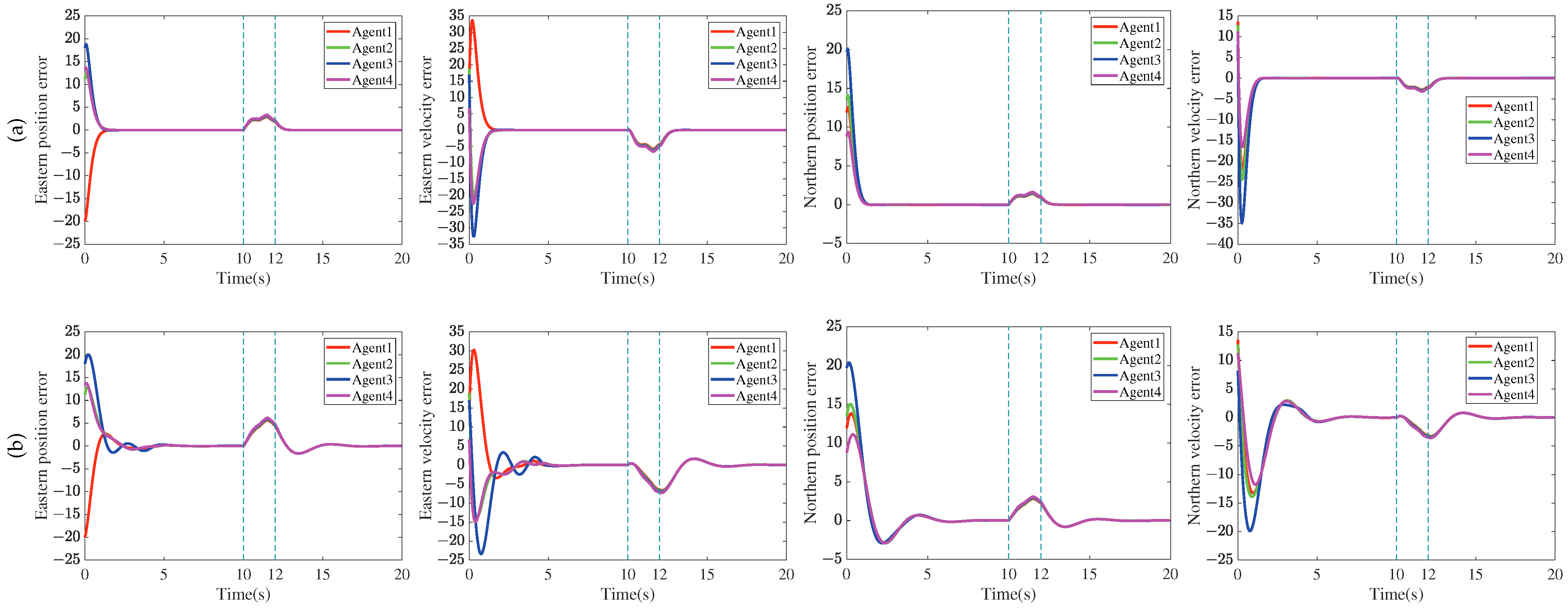
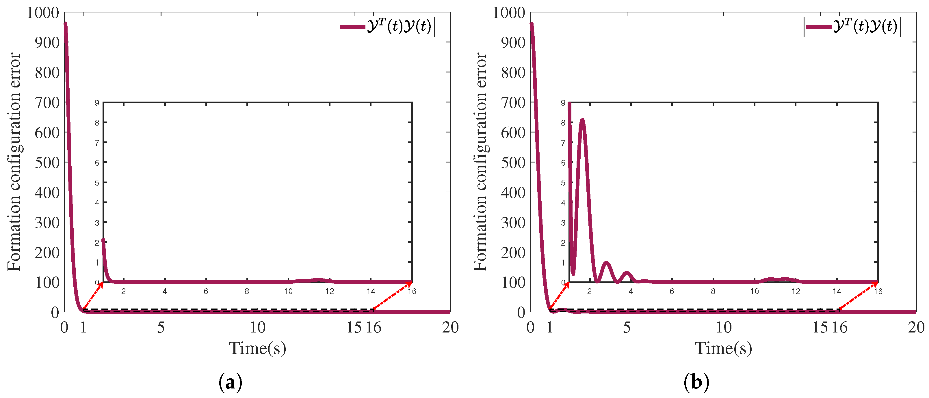
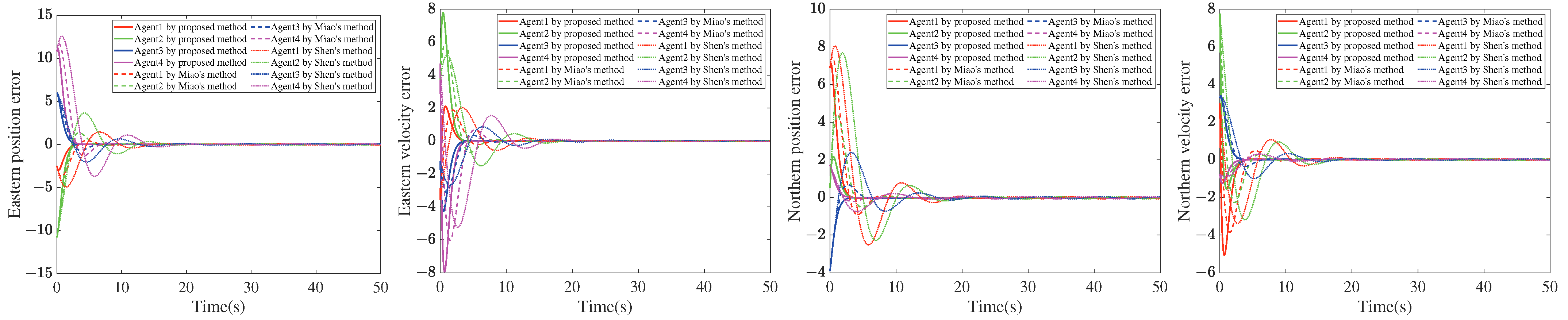
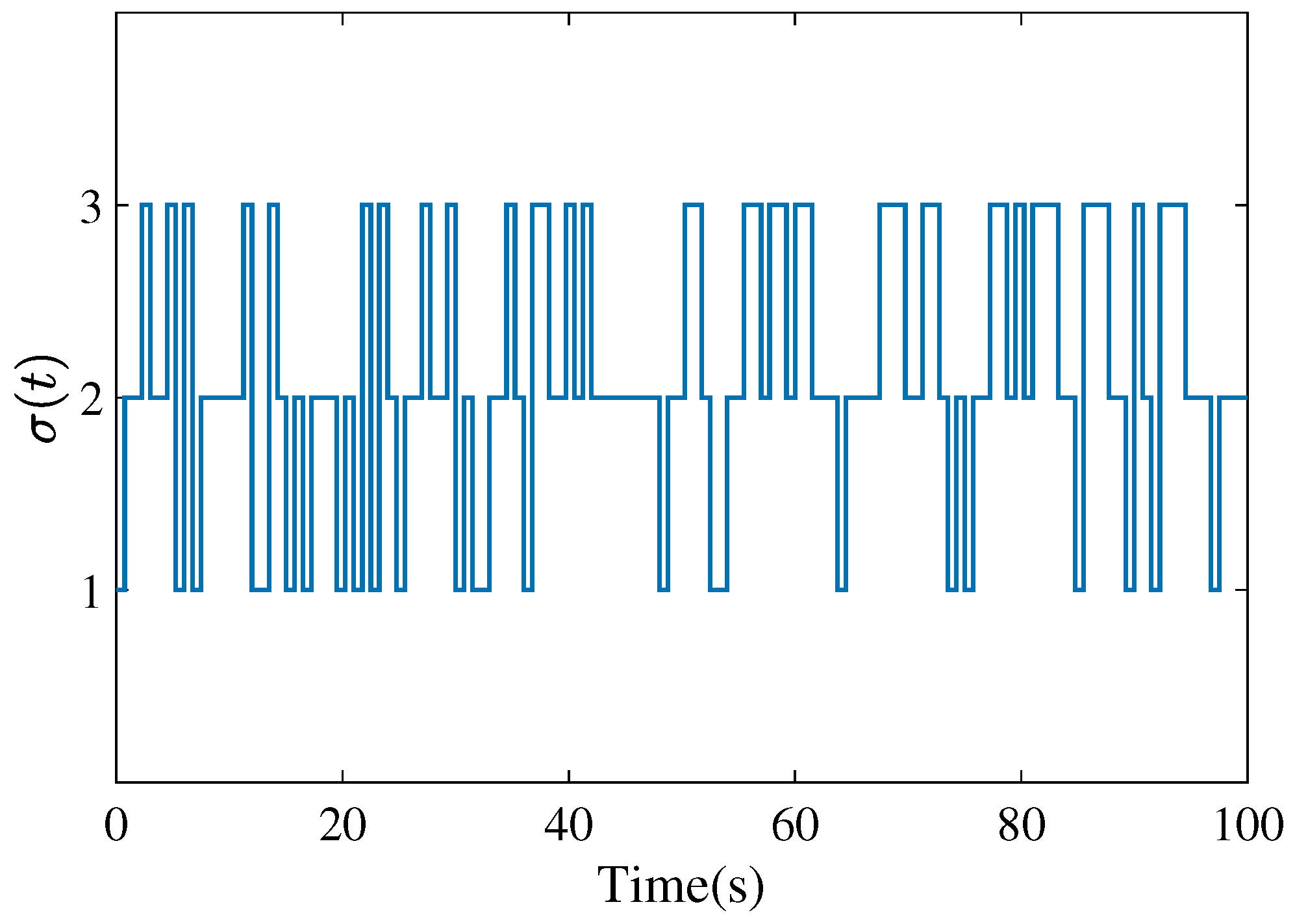
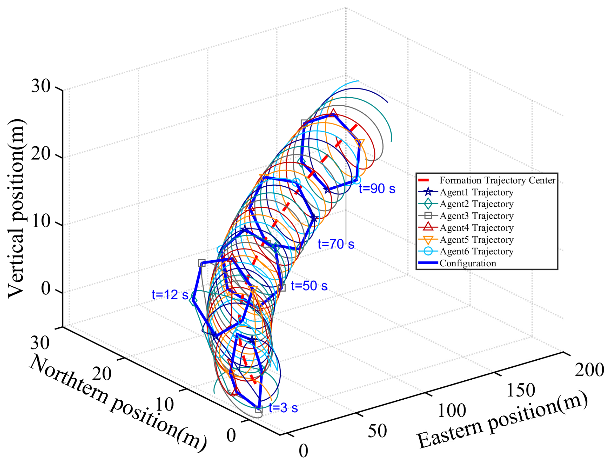
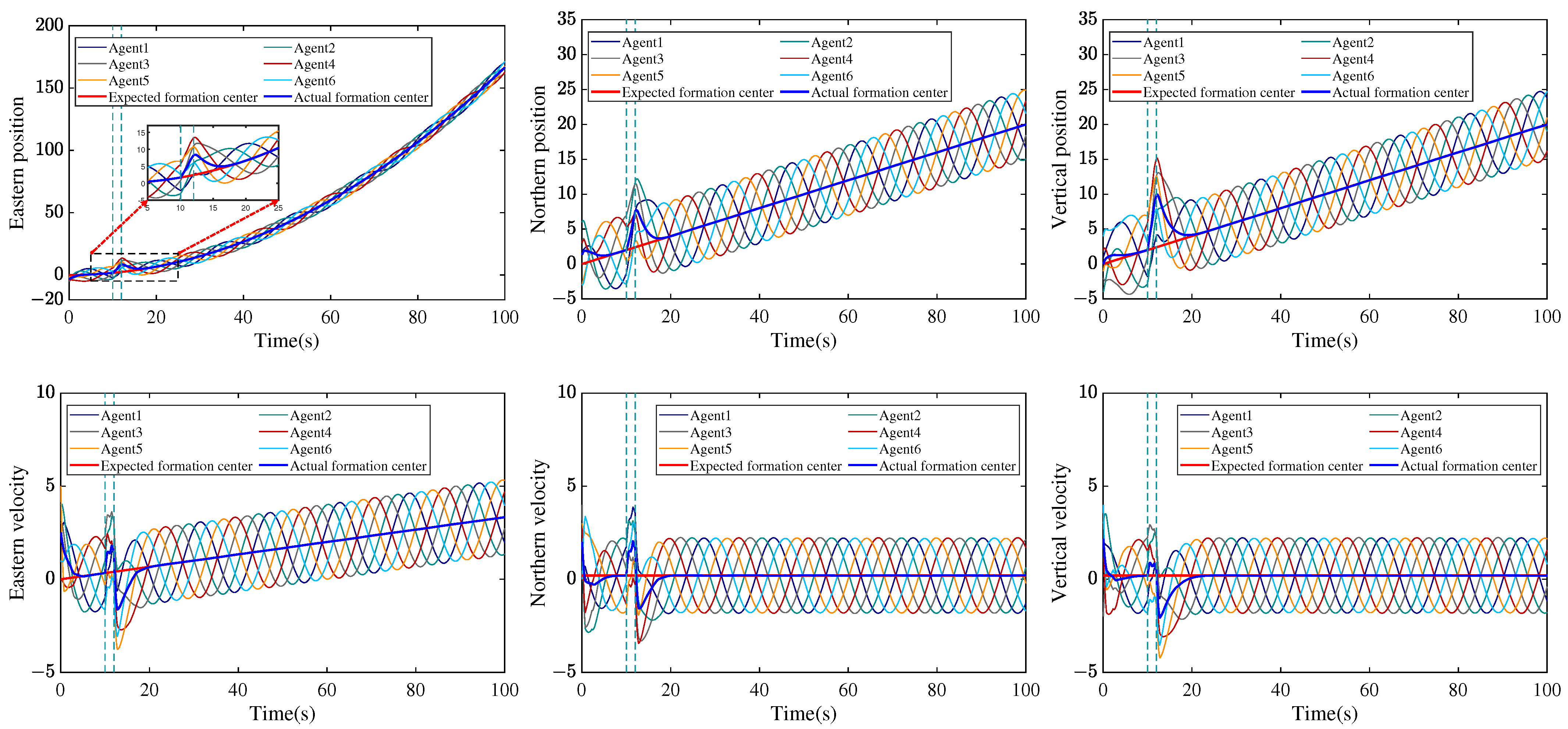
4. Simulation Results

In this section, the effectiveness of the proposed method is verified by three numerical simulations. Example 1 is compared with [11] in consideration of external disturbances and TVCDs under the same parameters, which proves the advancement of the method proposed in this paper. In comparison to the methods in [29,44], the superiority of the proposed method is proved in Example 2 when the MAS faces actuator faults under semi-Markov switching topologies. For the problems of TVCDs, uncertain parameters, external disturbances, actuator failures, and semi-Markov switching topologies, Example 3 substantiates the feasibility of the controller designed in Theorem 3.

Example 1.

Consider an MAS with four agents. The root node of the directed graph $\overline{\mathcal{G}}$ is agent 1. The model parameters of the MAS are as follows [11]:

$$\begin{array}{cc}\hfill & x_i=\left[\begin{array}{c}{x}_{i1}\\ x_{i2}\\ x_{i3}\\ x_{i4}\end{array}\right],\mathcal{A}=\left[\begin{array}{cccc}0& 1& 0& 0\\ 0& 0& 0& 0\\ 0& 0& 0& 1\\ 0& 0& 0& 0\end{array}\right],\overline{\mathcal{G}}=\left[\begin{array}{cccc}1& 0& 0& -1\\ -1& 2& 0& -1\\ 0& -1& 1& 0\\ -1& 0& 0& 1\end{array}\right],\hfill \\ \hfill & \mathcal{B}={\left[\begin{array}{cccc}0& 1& 0& 0\\ 0& 0& 0& 1\end{array}\right]}^T,\mathcal{H}=\left[\begin{array}{cccc}1& 0& 0& 0\\ 0& 0& 1& 0\end{array}\right],\mathcal{C}=I_4,E_{\hslash }=\mathbf{0},\hfill \end{array}$$

where $x_{i1},x_{i2},x_{i3},x_{i4}$ signify the eastern position, eastern velocity, northern position, and northern velocity of the ith agent, respectively. The initial state of each agent is designed as $x_1\left(0\right)={[-20,16,13,13.6]}^T$, $x_2\left(0\right)={[13,19,13.5,12]}^T$, $x_3\left(0\right)={[18,16,18.6,8.2]}^T$, and $x_4\left(0\right)={[11.6,6.8,8.8,12]}^T$.

The virtual formation center trajectory is set to $r\left(t\right)={[t/11,1/11,t^2/200,t/100]}^T$. The MAS’ TVF configuration is $h_i\left(t\right)={[h_{i10}\left(t\right),h_{i20}\left(t\right),h_{i30}\left(t\right),h_{i40}\left(t\right)]}^T$, where $h_{i10}\left(t\right)=1.8sin(0.6t+(i-1)\pi /2)$, $h_{i20}\left(t\right)=1.08cos(0.6t+(i-1)\pi /2)$, $h_{i30}\left(t\right)=1.1cos(0.7t+(i-1)\pi /2)$, $h_{i40}\left(t\right)=-0.77sin(0.7t+(i-1)\pi /2)$.

Choose $\overline{\mathcal{B}}=\left[\begin{array}{cccc}0& 1& 0& 0\\ 0& 0& 0& 1\end{array}\right]$ and $\tilde{\mathcal{B}}=\left[\begin{array}{cccc}1& 0& 0& 0\\ 0& 0& 1& 0\end{array}\right]$ to satisfy (15). In addition, according to (14), we have ${\psi }_i\left(t\right)={[-0.648sin(0.6t+(i-1)\pi /2),-0.539cos(0.7t+(i-1)\pi /2)+1/100]}^T$.

Let the disturbance attenuation parameter $\gamma =12.5$, $c_4=0.84$, ${\delta }_1=0.8$. Select the TVCDs as $\tau \left(t\right)=0.2+0.2\sin (t-{\displaystyle \frac{\pi }{2}})$, and $\overline{\tau }=0.4$, $\overline{\mu }=0.2$. The external disturbances are designed as ${\omega }_i\left(t\right)={[0.5\overline{\omega }\left(t\right),0.32\overline{\omega }\left(t\right),0.24\overline{\omega }\left(t\right),0.18\overline{\omega }\left(t\right)]}^T\times (20+i)/20$, where

$$\overline{\omega }\left(t\right)=\left\{\begin{array}{cc}10,\hfill & 10\le t\le 10.5\hfill \\ 8,\hfill & 10.5\le t\le 11\hfill \\ 12,\hfill & 11\le t\le 11.5\hfill \\ 6,\hfill & 11.5\le t\le 12\hfill \\ 0,\hfill & \mathrm{others}.\hfill \end{array}\right.$$

Then, by solving LMIs (26), we can obtain the feedback gain matrices

$$\begin{array}{cc}\hfill {\mathcal{K}}_{\alpha =\overline{\mathcal{G}},1}& =\left[\begin{array}{cccc}16.0204& 7.2694& 0& 0\\ 0& 0& 16.0204& 7.2694\end{array}\right],\hfill \\ \hfill {\mathcal{K}}_{\alpha =\overline{\mathcal{G}},2}& =\left[\begin{array}{cccc}-0.3360& 0.0699& 0& 0\\ 0& 0& -0.3360& 0.0699\end{array}\right].\hfill \end{array}$$

Figure 1 depicts the eastern position trajectory tracking errors, eastern velocity trajectory tracking errors, northern position trajectory tracking errors, and northern velocity trajectory tracking errors of the four agents from $t=0$ s to $t=20$ s in the face of TVCDs and external disturbances imposed within $t=10$ s and $t=12$ s. The upper four graphs show the trajectory tracking errors applying this paper’s method and the lower four demonstrate errors using the approach in [11]. The tracking errors of agents 1–4 are represented by red, green, blue, and purple curves, respectively. The control effect of TVF trajectory tracking can be seen from the variation in four error curves in each subgraph and the speed of convergence to 0. Figure 2 shows the formation performance function curves under the condition of MASs suffering from TVCDs and external disturbances imposed from $t=10$ s to $t=12$ s, in which the subgraph pointed by the red dash-dot line represents the enlarged view from $t=1$ s to $t=16$ s. The subgraph (a) is the formation performance function curve of the method proposed in this paper, and (b) is the method in [11]. From Figure 1 and Figure 2, it is not difficult to see that the controller designed by the method proposed in this paper is effective enough to resist the influence of TVCDs and external disturbances on the MAS. Comparing with the method in reference [11], Figure 1 shows that the position and velocity error curves can converge from the initial state to 0 in $t=2$ s by the proposed method, while error curves converge to 0 after $t=5$ s by [11]. In addition, for the external disturbances imposed at $t=10$ s to $t=12$ s, the proposed method can quickly suppress it and the error fluctuation is smaller, while the suppression effect of [11] on the interference is not obvious, resulting in large fluctuations. From the formation performance function of Figure 2, the proposed method converges faster, has better performance, and has stronger suppression in the face of external disturbances. Therefore, the proposed method in this paper can effectively suppress TVCDs and external disturbances, i.e., it has stronger robustness.

Remark 6.

The $\overline{\tau }$ calculated in [11] is 0.134 s, while that selected in this paper is 0.4 s. However, the results of [11] can still converge. This demonstrates that the calculation of $\overline{\tau }$ in [11] is more conservative, and the proposed method can allow bigger CDs and reduce conservatism.

Example 2.

In this Example, the TVF problem of an MAS with actuator faults under semi-Markov switching topologies is investigated, which illustrates the superiority of the proposed method by comparing it with the methods in [29,44].

Consider an MAS with four agents, whose system parameters $x_i,\mathcal{A},\mathcal{B},\mathcal{C},\mathcal{H},E_{\hslash }$, $h_i\left(t\right),\overline{\mathcal{B}},\tilde{\mathcal{B}}$ are the same as Example 1. The initial state of each agent is set to $x_1\left(0\right)={[-2.5,-2,8,3]}^T$, $x_2\left(0\right)={[-9,4.2,0.5,7]}^T$, $x_3\left(0\right)={[6,-1.8,-5,3.3]}^T$, $x_4\left(0\right)={[9,5.2,1.7,0]}^T$. The virtual formation center trajectory is designed as $r\left(t\right)=[t/2,1/2,t^2/4,t/2]$. Thus from (14), we can derive the auxiliary function ${\psi }_i\left(t\right)={[-0.648sin(0.6t+(i-1)\pi /2),-0.539cos(0.7t+(i-1)\pi /2)+1/2]}^T$. Set $\gamma =10.5,c_4=0.6,{\delta }_1={\delta }_2={\delta }_3=0.25$, $\tau \left(t\right)=0$, and ${\omega }_i\left(t\right)=\mathbf{0}$.

In this paper, the topology-switching Laplacian matrices of the semi-Markov stochastic process $\mathcal{P}\left(t\right)$ (state space is $S=1,2,3$, initial state is $\sigma \left(0\right)=1$) are selected as follows:

$$\begin{array}{c}\hfill {\mathcal{L}}_1=\left[\begin{array}{cccc}1& 0& 0& -1\\ -1& 1& 0& 0\\ 0& -1& 1& 0\\ 0& 0& -1& 1\end{array}\right],{\mathcal{L}}_2=\left[\begin{array}{cccc}0& 0& 0& 0\\ -1& 1& 0& 0\\ -1& -1& 2& 0\\ 0& 0& -1& 1\end{array}\right],{\mathcal{L}}_3=\left[\begin{array}{cccc}0& 0& 0& 0\\ -1& 2& 0& -1\\ 0& 0& 1& -1\\ -1& 0& 0& 1\end{array}\right].\end{array}$$

On the basics of Remark 4, the transition rate matrix of $\mathcal{P}\left(t\right)$ is selected as $0.1\le {\lambda }_{12}\left(h\right)\le 0.65$, $0.1\le {\lambda }_{13}\left(h\right)\le 0.9$, $0.4\le {\lambda }_{21}\left(h\right)\le 1.2$, $0.6\le {\lambda }_{23}\left(h\right)\le 1.41$, $1.06\le {\lambda }_{31}\left(h\right)\le 2.2$, $1.2\le {\lambda }_{32}\left(h\right)\le 2.2$. The parameters of failures are chosen as

$$\begin{array}{cc}\hfill & {\tilde{\rho }}_{ij}=0.8,\mathbb{E}\{{\xi }_{ij}\left(k\right)=1\}=0.3(i=1,2,3,4,j=1,2),\hfill \\ & \left\{\begin{array}{c}0.65\le {\rho }_{ij}\le 0.8,{\xi }_{ij}\left(k\right)=1\hfill \\ 0.8\le {\overline{\rho }}_{ij}\le 0.9,{\xi }_{ij}\left(k\right)=0\hfill \end{array}\right.i=1,2,3,4.\hfill \end{array}$$

Based on the above analysis, we can achieve the desired TVF by solving the LMIs in Theorem 3. In light of utilizing references [29,44] and the proposed methods to design the controller, the comparative tracking errors and the formation performance results in Figure 3 and Figure 4, respectively, can be obtained.

By utilizing the controllers designed by [29,44] and the proposed method, Figure 3 illustrates the eastern position, eastern velocity, northern position, and northern velocity tracking errors of an MAS with actuator faults under semi-Markov switching topologies. Concurrently, the formation performance curves are presented in Figure 4. From Figure 3, it is not difficult to see that compared with the methods in [29,44], the tracking errors from the controller designed in this paper converge to zero more rapidly and exhibit less fluctuation when confronted with actuator faults under semi-Markov switching topologies. Furthermore, Figure 4 suggests that the proposed method offers superior formation performance relative to the methods in [29,44] for achieving TVF and maintaining the formation shape more effectively. Based on the aforementioned analysis, we can conclude that the method proposed in this paper has faster convergence speed and stronger robustness to realize the TVF of MASs in the face of actuator faults under semi-Markov switching topologies.

Example 3.

An MAS suffering from uncertain parameters, TVCDs, external disturbances, semi-Markov switching topologies, and actuator faults problems is considered, which consists of six agents. The model parameters of the MAS are designed as

$$\begin{array}{cc}\hfill & x_i={\left[\begin{array}{c}{x}_{i1}\\ x_{i2}\\ x_{i3}\\ x_{i4}\\ x_{i5}\\ x_{i6}\end{array}\right]}^T,\mathcal{A}+\Delta \mathcal{A}=\left[\begin{array}{cccccc}0& 1& 0& 0& 0& 0\\ 0& 0& 0& 0& 0& {\Delta }_1\\ 0& 0& 0& 1+{\Delta }_2& 0& 0\\ 0& 0& 0& 0& 0& 0\\ 0& 0& 0& 0& 0& 1+{\Delta }_3\\ 0& 0& 0& 0& 0& 0\end{array}\right],\mathcal{B}=\left[\begin{array}{ccc}0& 0& 0\\ 1& 0& 0\\ 0& 0& 0\\ 0& 1& 0\\ 0& 0& 0\\ 0& 0& 1\end{array}\right]\hfill \\ \hfill & \mathcal{H}=\left[\begin{array}{cccccc}1& 0& 0& 0& 0& 0\\ 0& 0& 1& 0& 0& 0\\ 0& 0& 0& 0& 1& 0\end{array}\right],\begin{array}{c}\mathcal{C}=I_6,{\Delta }_1={\Delta }_3=sin\left(t\right),\hfill \\ {\Delta }_2=cos\left(t\right),\hfill \end{array}\hfill \\ \hfill & E_{\hslash }=G_{\hslash a}=\mathrm{diag}\{0.5,0.5,0.5,0.5,0.5,0.5\}.\hfill \end{array}$$

where $x_{i1},x_{i3},x_{i5},x_{i2},x_{i4},x_{i6}$ signify the eastern, northern, and vertical position and eastern, northern, and vertical velocity of the ith agent, respectively. The initial state is set to $x_{10}={[-3,2,2,0,1,2]}^T$, $x_{20}={[-3,4,6,2,-4,3]}^T$, $x_{30}={[-5,3,3,4,-2,-2]}^T$, $x_{40}={[-4,0,3,3,2,2]}^T$, $x_{50}={[-2,5,-3,3,-1,4]}^T$, $x_{60}={[-3,1,-3,0,4,4]}^T$. $r\left(t\right)=[t^2/60,t/30,$${t/5,1/5,t/5,1/5]}^T$.

The TVF configuration is selected as $h_i\left(t\right)={[h_{i1}\left(t\right),h_{21}\left(t\right),h_{i3}\left(t\right),h_{i4}\left(t\right),h_{i5}\left(t\right),h_{i6}\left(t\right)]}^T$, where $h_{i1}\left(t\right)=5sin(0.4t+(i-1)\pi /3)$, $h_{i2}\left(t\right)=2cos(0.4t+(i-1)\pi /3)$, $h_{i3}\left(t\right)=5cos(0.4t+(i-1)\pi /3)$, $h_{i4}\left(t\right)=-2sin(0.4t+(i-1)\pi /3)$, $h_{i5}\left(t\right)=5sin(0.4t+(i-1)\pi /3)$ and $h_{i6}\left(t\right)=2cos(0.4t+(i-1)\pi /3)$. According to (15), picking the nonsingular matrix $\widehat{\mathcal{B}}={[{\overline{\mathcal{B}}}^T,{\tilde{\mathcal{B}}}^T]}^T$ and

$$\overline{\mathcal{B}}=\left[\begin{array}{cccccc}0& 1& 0& 0& 0& 0\\ 0& 0& 0& 1& 0& 0\\ 0& 0& 0& 0& 0& 1\end{array}\right],\tilde{\mathcal{B}}=\left[\begin{array}{cccccc}1& 0& 0& 0& 0& 0\\ 0& 0& 1& 0& 0& 0\\ 0& 0& 0& 0& 1& 0\end{array}\right].$$

Thus, we can obtain the auxiliary function ${\psi }_i\left(t\right)=[-0.8sin(0.4t+(i-1)\pi /3)+1/30$, $-0.8cos(0.4t+(i-1)\pi /3)$, ${-0.8sin(0.4t+(i-1)\pi /3)]}^T$ from (14).

Let $\gamma =5.5$, $c_4=0.8$, ${\delta }_1={\delta }_2={\delta }_3=0.1$. $\tau \left(t\right)=0.6+0.6\sin (t-\pi /2)$, and $\overline{\tau }=1.2$, $\overline{\mu }=0.6$.

The external disturbances are devised as ${\omega }_i\left(t\right)=\tilde{\omega }\left(t\right)\times (20+i)/20$, where $\tilde{\omega }\left(t\right)={[0.18\overline{\omega }\left(t\right),0.24\overline{\omega }\left(t\right),0.12\overline{\omega }\left(t\right),0.27\overline{\omega }\left(t\right),0.31\overline{\omega }\left(t\right),0.16\overline{\omega }\left(t\right)]}^T$ and $\overline{\omega }\left(t\right)$ has been defined in Example 1.

In this paper, we utilize the semi-Markov process $\mathcal{P}\left(t\right)$ to model the switching communication topologies. Its finite state space is $S=\{1,2,3\}$ and initial state is $\sigma \left(0\right)=1$. Furthermore, the communication topologies of the MAS (2) are constructed as ${\mathcal{G}}_i(i\in S)$, as depicted in Figure 5, where the numbers 1 to 6 in the figure represent the 1st to 6th agents. According to Remark 4, the transition rate matrix is chosen such that $0.2\le {\lambda }_{12}\left(h\right)\le 0.8$, $0.1\le {\lambda }_{13}\left(h\right)\le 0.6$, $0.5\le {\lambda }_{21}\left(h\right)\le 1.1$, $0.5\le {\lambda }_{23}\left(h\right)\le 1.32$, $1.0\le {\lambda }_{31}\left(h\right)\le 1.9$, $1.2\le {\lambda }_{32}\left(h\right)\le 2.1$. Figure 6 reflects the topologies switching of the semi-Markov stochastic process from $t=0$ s to $t=100$ s.

The parameters of failures are defined as

$$\begin{array}{cc}\hfill & {\tilde{\rho }}_{ij}=0.8,\mathbb{E}\{{\xi }_{ij}\left(k\right)=1\}=0.3(i=1,2,3,4,5,6,j=1,2,3),\hfill \\ & \left\{\begin{array}{c}0.65\le {\rho }_{ij}\le 0.8,{\xi }_{ij}\left(k\right)=1\hfill \\ 0.8\le {\overline{\rho }}_{ij}\le 0.9,{\xi }_{ij}\left(k\right)=0\hfill \end{array}\right.i=1,2,3,\hfill \\ & \left\{\begin{array}{c}0.7\le {\rho }_{ij}\le 0.8,{\xi }_{ij}\left(k\right)=1\hfill \\ 0.8\le {\overline{\rho }}_{ij}\le 0.9,{\xi }_{ij}\left(k\right)=0\hfill \end{array}\right.i=4,5,6.\hfill \end{array}$$

Based on the above given parameters, the controller gain matrices in Theorem 3 can be derived. They are presented as follows:

$$\begin{array}{cc}\hfill {\mathcal{K}}_{11}& =\left[\begin{array}{cccccc}1.2673& 2.5783& 0& 0& 0& 0\\ 0& 0& 1.2673& 2.5783& 0& 0\\ 0& 0& 0& 0& 0.9958& 2.4141\end{array}\right],\hfill \end{array}$$

$$\begin{array}{cc}\hfill {\mathcal{K}}_{12}& =\left[\begin{array}{cccccc}0.0022& 0.0164& 0& 0& 0& 0\\ 0& 0& 0.0022& 0.0164& 0& 0\\ 0& 0& 0& 0& 0.0020& 0.0161\end{array}\right],\hfill \\ \hfill {\mathcal{K}}_{21}& =\left[\begin{array}{cccccc}0.6254& 1.5878& 0& 0& 0& 0\\ 0& 0& 0.6254& 1.5878& 0& 0\\ 0& 0& 0& 0& 0.4757& 1.5334\end{array}\right],\hfill \\ \hfill {\mathcal{K}}_{22}& =\left[\begin{array}{cccccc}-0.0016& 0.0136& 0& 0& 0& 0\\ 0& 0& -0.0016& 0.0136& 0& 0\\ 0& 0& 0& 0& -0.0006& 0.0149\end{array}\right],\hfill \\ \hfill {\mathcal{K}}_{31}& =\left[\begin{array}{cccccc}0.3330& 1.0448& 0& 0& 0& 0\\ 0& 0& 0.3330& 1.0448& 0& 0\\ 0& 0& 0& 0& 0.2605& 1.0671\end{array}\right],\hfill \\ \hfill {\mathcal{K}}_{32}& =\left[\begin{array}{cccccc}-0.0011& 0.0044& 0& 0& 0& 0\\ 0& 0& -0.0011& 0.0044& 0& 0\\ 0& 0& 0& 0& -0.0004& 0.0059\end{array}\right].\hfill \end{array}$$

By implementing the above controller gains into the error system, Figure 7, Figure 8 and Figure 9 depict the trajectory tracking 3D diagram, the trajectories on eastern, northern, and vertical position and velocity, and curves of tracking formation performance of an MAS with multi-coupling problems, respectively. From Figure 7 and Figure 8, we can draw the following conclusions: (1) The formation configuration composed of six agents is a regular hexagon, and the trajectory center can be tracked accurately. (2) Under nonzero initial conditions, the actual formation center of the MAS in the eastern, northern, and vertical directions can converge to the expected formation center within $t=8$ s. In addition, the severe external disturbances from $t=10$ s to $t=12$ s can be well suppressed by the proposed controller to ensure that TVF is maintained. Figure 9 demonstrates that the proposed method can still make MASs maintain a good tracking formation performance even under the influence of stochastic switching topologies. In summary, although the system will be affected by multi-coupling constraints simultaneously, the controller designed by the method proposed in this paper can effectively suppress these hybrid problems, so as to achieve the control objective of TVF trajectory tracking. Thus the validity of Theorem 3 is demonstrated. It is worth noting that, compared with the existing research in the field of TVF, we consider the above five coupling problems in Table 1 for the first time in Example 3.

5. Discussion

In this study, the fault-tolerant time-varying formation trajectory tracking control problem is addressed by a novel distributed state-feedback control protocol for uncertain multi-agent systems with external disturbances subject to time-varying communication delays under semi-Markov switching topologies. Compared with the previous studies [11,29,44], the proposed method significantly improves the upper bound of the delays tolerated by MASs based on the Lyapunov–Krasovskii stability theory and the reciprocally convex combination theory. It also enhances the convergence speed and robustness of MASs by using the $H_{\infty }$ control approach. Furthermore, the proposed method constructs a failure distribution based on the characteristics of actuator faults in practice and introduces a semi-Markov stochastic process based on convex functions to model switching topologies. More importantly, we realize the TVF trajectory tracking control of MASs with the five tight coupling problems mentioned in the above discussion for the first time, which means more practical significance and wider application value.

However, the MASs model selected in the current research work is a general linear model, whereas most systems in the real environment are nonlinear models. Additionally, the current research is still limited to computer numerical simulations without validation in real-world environments. Future research will aim to extend the proposed method and apply it to three-dimensional real-world settings and conduct comprehensive physical experiments to verify its effectiveness and robustness in practical applications. For instance, research on TVF trajectory tracking control for multi-UAV systems will be carried out, and physical flight experiments will be conducted using multiple quadrotor drones.

6. Conclusions

In this paper, the problem of fault-tolerant TVF trajectory tracking control for uncertain MASs with external disturbances subject to TVCDs under SMSTs has been studied. On the basics of the characteristics of actuator failures, a failure distribution has been established. A novel distributed state-feedback controller has been designed for MASs to suppress the influence of different constraints. The TVF issue has been converted into the problem about asymptotic stability. To derive the criterion and reduce the conservatism, an advanced LK functional has been constructed and the reciprocally convex combination theory has been applied. In addition, the stability criteria were presented in the form of matrix inequalities, and the controller gain matrices could be obtained by solving LMIs. Ultimately, the effectiveness and superiority of the proposed method have been presented through three simulation examples. TVF trajectory tracking control of nonlinear multi-UAV systems with time-varying delays and external disturbances under semi-Markov switching topologies will be our work interest in the future.

References

1. Yu, Y.; Chen, J.; Zheng, Z.; Yuan, J. Distributed Finite-Time ESO-Based Consensus Control for Multiple Fixed-Wing UAVs Subjected to External Disturbances. Drones 2024, 8, 260. [Google Scholar] [CrossRef]
2. Yang, Y.; He, Y. Containment Control for Second-Order Multi-Agent Systems with Time-Varying Delays via Variable-Augmented-Based Free-Weighting Matrices. J. Franklin Inst. 2024, 361, 106816. [Google Scholar] [CrossRef]
3. Cheng, H.; Huang, J. Adaptive Robust Bearing-Based Formation Control for Multi-Agent Systems. Automatica 2024, 162, 111509. [Google Scholar] [CrossRef]
4. Huang, Y.; Fang, W.; Chen, Z.; Li, Y.; Yang, C. Flocking of Multiagent Systems with Nonuniform and Nonconvex Input Constraints. IEEE Trans. Autom. Control 2023, 68, 4329–4335. [Google Scholar] [CrossRef]
5. Xiao, H.; Li, Z.; Philip Chen, C.L. Formation Control of Leader–Follower Mobile Robots’ Systems Using Model Predictive Control Based on Neural-Dynamic Optimization. IEEE Trans. Ind. Electron. 2016, 63, 5752–5762. [Google Scholar] [CrossRef]
6. Gu, N.; Wang, D.; Peng, Z.; Liu, L. Distributed Containment Maneuvering of Uncertain Under-Actuated Unmanned Surface Vehicles Guided by Multiple Virtual Leaders with a Formation. Ocean Eng. 2019, 187, 105996. [Google Scholar] [CrossRef]
7. Lin, J.; Hwang, K.; Wang, Y. A Simple Scheme for Formation Control Based on Weighted Behavior Learning. IEEE Trans. Neural Netw. Learn. Syst. 2014, 25, 1033–1044. [Google Scholar] [CrossRef]
8. Koru, A.T.; Ramírez, A.; Sarsılmaz, S.B.; Sipahi, R.; Yucelen, T.; Dogan, K.M. Containment Control of Multi-Human Multi-Agent Systems Under Time Delays. IEEE Trans. Syst. Man Cybern. Syst. 2024, 54, 3344–3356. [Google Scholar] [CrossRef]
9. Kang, Y.; Luo, D.; Xin, B.; Cheng, J.; Yang, T.; Zhou, S. Robust Leaderless Time-Varying Formation Control for Nonlinear Unmanned Aerial Vehicle Swarm System with Communication Delays. IEEE Trans. Cybern. 2023, 53, 5692–5705. [Google Scholar] [CrossRef] [PubMed]
10. Shahbazi, B.; Malekzadeh, M.; Koofigar, H.R. Robust Constrained Attitude Control of Spacecraft Formation Flying in the Presence of Disturbances. IEEE Trans. Aerosp. Electron. Syst. 2017, 53, 2534–2543. [Google Scholar] [CrossRef]
11. Cheng, J.; Kang, Y.; Xin, B.; Zhang, Q.; Mao, K.; Zhou, S. Time-Varying Trajectory Tracking Formation H Control for Multiagent Systems with Communication Delays and External Disturbances. IEEE Trans. Syst. Man Cybern. Syst. 2022, 52, 4311–4323. [Google Scholar] [CrossRef]
12. Xu, Z.; Li, Y.; Zhan, X.; Yan, H.; Han, Y. Time-Varying Formation of Uncertain Nonlinear Multi-Agent Systems via Adaptive Feedback Control Approach with Event-Triggered Impulsive Estimator. Appl. Math. Comput. 2024, 475, 128707. [Google Scholar] [CrossRef]
13. Guo, H.; Meng, M.; Feng, G. Lyapunov-Based Output Containment Control of Heterogeneous Multi-Agent Systems with Markovian Switching Topologies and Distributed Delays. IEEE/CAA J. Autom. Sin. 2023, 10, 1421–1433. [Google Scholar] [CrossRef]
14. Li, M.; Deng, F. Necessary and Sufficient Conditions for Consensus of Continuous-Time Multiagent Systems with Markovian Switching Topologies and Communication Noises. IEEE Trans. Cybern. 2020, 50, 3264–3270. [Google Scholar] [CrossRef]
15. Ma, L.; Wang, Z.; Han, Q.; Liu, Y. Consensus Control of Stochastic Multi-Agent Systems: A Survey. Sci. China Inf. Sci. 2017, 60, 120201. [Google Scholar] [CrossRef]
16. Mu, X.; Hu, Z. Stability Analysis for Semi-Markovian Switched Singular Stochastic Systems. Automatica 2020, 118, 109014. [Google Scholar] [CrossRef]
17. Dai, J.; Guo, G. Event-Triggered Leader-Following Consensus for Multi-Agent Systems with Semi-Markov Switching Topologies. Inform. Sci. 2018, 459, 290–301. [Google Scholar] [CrossRef]
18. Liang, H.; Zhang, L.; Sun, Y.; Huang, T. Containment Control of Semi-Markovian Multiagent Systems with Switching Topologies. IEEE Trans. Syst. Man Cybern. Syst. 2021, 51, 3889–3899. [Google Scholar] [CrossRef]
19. He, M.; Mu, J.; Mu, X. H Leader-Following Consensus of Nonlinear Multi-Agent Systems under Semi-Markovian Switching Topologies with Partially Unknown Transition Rates. Inform. Sci. 2020, 513, 168–179. [Google Scholar] [CrossRef]
20. Su, L.; Qi, Y.; Shen, H. Event-Based Fault-Tolerant H Synchronization for Inertial Neural Networks via a Semi-Markov Jump Approach. J. Franklin Inst. 2023, 360, 11829. [Google Scholar] [CrossRef]
21. Li, K.; Ding, S.X.; Zheng, W.X.; Hua, C.C. Global Distributed Fault-Tolerant Consensus Control of Nonlinear Delayed Multiagent Systems with Hybrid Faults. IEEE Trans. Autom. Control 2024, 69, 1967–1974. [Google Scholar] [CrossRef]
22. Niederlinski, A. A Heuristic Approach to the Design of Linear Multivariable Interacting Control Systems. Automatica 1971, 7, 691–701. [Google Scholar] [CrossRef]
23. Hu, H.; Liu, L.; Wang, Y.; Cheng, Z.; Luo, Q. Active Fault-Tolerant Attitude Tracking Control with Adaptive Gain for Spacecrafts. Aerosp. Sci. Technol. 2020, 98, 105706. [Google Scholar] [CrossRef]
24. Ke, C.; Cai, K.Y.; Quan, Q. Uniform Passive Fault-Tolerant Control of a Quadcopter with One, Two, or Three Rotor Failure. IEEE Trans. Rob. 2023, 39, 4297–4311. [Google Scholar] [CrossRef]
25. Zhao, W.; Liu, H.; Wan, Y. Data-Driven Fault-Tolerant Formation Control for Nonlinear Quadrotors under Multiple Simultaneous Actuator Faults. Syst. Control Lett. 2021, 158, 105063. [Google Scholar] [CrossRef]
26. Guo, X.; Wei, G.; Ding, D. Fault-Tolerant Consensus Control for Discrete-Time Multi-Agent Systems: A Distributed Adaptive Sliding-Mode Scheme. IEEE Trans. Circuits Syst. II Express Briefs 2023, 70, 2515–2519. [Google Scholar] [CrossRef]
27. Ruan, Z.; Yang, Q.; Ge, S.S.; Sun, Y. Adaptive Fuzzy Fault Tolerant Control of Uncertain MIMO Nonlinear Systems with Output Constraints and Unknown Control Directions. IEEE Trans. Fuzzy Syst. 2022, 30, 1224–1238. [Google Scholar] [CrossRef]
28. Yin, S.; Gao, H.; Qiu, J.; Kaynak, O. Adaptive Fault-Tolerant Control for Nonlinear System with Unknown Control Directions Based on Fuzzy Approximation. IEEE Trans. Syst. Man Cybern. Syst. 2017, 47, 1909–1918. [Google Scholar] [CrossRef]
29. Miao, K.; Li, J.; Chen, Y.; Xu, S. Finite-Time Fault-Tolerant Consensus for Leader-Following Multi-Agent Systems with Semi-Markov Switching Topologies. Int. J. Control 2022, 97, 373–386. [Google Scholar] [CrossRef]
30. Zhou, Y.; Chang, X.; Park, J.H. Quantized Asynchronous Filtering for Fuzzy Semi-Markov Switching Systems with Multiple Stochastic Delays Under Deception Attacks. IEEE Trans. Fuzzy Syst. 2024, 32, 2378–2389. [Google Scholar] [CrossRef]
31. Zhou, T.; Liu, C.; Wang, W. Nonfragile Robust H Containment Control for Multi-Agent Systems with a Time-Varying Delay. J. Franklin Inst. 2024, 361, 106732. [Google Scholar] [CrossRef]
32. Ren, W.; Beard, R. Consensus Seeking in Multiagent Systems under Dynamically Changing Interaction Topologies. IEEE Trans. Autom. Control 2005, 50, 655–661. [Google Scholar] [CrossRef]
33. Yang, R.; Liu, L.; Feng, G. Leader-Following Output Consensus of Heterogeneous Uncertain Linear Multiagent Systems with Dynamic Event-Triggered Strategy. IEEE Trans. Syst. Man Cybern. Syst. 2022, 52, 1626–1637. [Google Scholar] [CrossRef]
34. Dong, X.; Yu, B.; Shi, Z.; Zhong, Y. Time-Varying Formation Control for Unmanned Aerial Vehicles: Theories and Applications. IEEE Trans. Control Syst. Technol. 2015, 23, 340–348. [Google Scholar] [CrossRef]
35. Wang, A.; Fei, M.; Song, Y. A Novel Scalable and Reliable Control for DC Microgrids with Varying Number of Agents. IEEE Trans. Cybern. 2024, 54, 4962–4972. [Google Scholar] [CrossRef]
36. Peng, X.; He, Y. Consensus of Multiagent Systems with Time-Varying Delays and Switching Topologies Based on Delay-Product-Type Functionals. IEEE Trans. Cybern. 2024, 54, 101–110. [Google Scholar] [CrossRef] [PubMed]
37. Yang, J.; Zhong, Q.; Wang, Y.; Shi, K.; Zhong, S. Nonfragile Memory-Based PD-Like Sampled-Data Consensus Control for Nonlinear Multiagent Systems with Time-Varying Communication Delays. IEEE Trans. Syst. Man Cybern. Syst. 2023, 53, 4370–4380. [Google Scholar] [CrossRef]
38. Cao, Y.; Lam, J. Robust H Control of Uncertain Markovian Jump Systems with Time-Delay. IEEE Trans. Autom. Control 2000, 45, 77–83. [Google Scholar] [CrossRef]
39. Boyd, S.; El Ghaoui, L.; Feron, E.; Balakrishnan, V. Linear Matrix Inequalities in System and Control Theory; Studies in Applied and Numerical Mathematics; Society for Industrial and Applied Mathematics: Philadelphia, PA, USA, 1994. [Google Scholar] [CrossRef]
40. Chen, J.; Park, J.H.; Xu, S.; Zhang, B. A Survey of Inequality Techniques for Stability Analysis of Time-Delay Systems. Int. J. Robust Nonlinear Control 2022, 32, 6412–6440. [Google Scholar] [CrossRef]
41. Park, P.; Ko, J.W.; Jeong, C. Reciprocally Convex Approach to Stability of Systems with Time-Varying Delays. Automatica 2011, 47, 235–238. [Google Scholar] [CrossRef]
42. Yang, G.; Wang, J.L. Non-Fragile H Control for Linear Systems with Multiplicative Controller Gain Variations. Automatica 2001, 37, 727–737. [Google Scholar] [CrossRef]
43. Shen, H.; Park, J.H.; Wu, Z.G.; Zhang, Z. Finite-Time H∞ Synchronization for Complex Networks with Semi-Markov Jump Topology. Commun. Nonlinear Sci. Numer. Simul. 2015, 24, 40–51. [Google Scholar] [CrossRef]
44. Shen, H.; Wang, Y.; Xia, J.; Park, J.H.; Wang, Z. Fault-Tolerant Leader-Following Consensus for Multi-Agent Systems Subject to Semi-Markov Switching Topologies: An Event-Triggered Control Scheme. Nonlinear Anal. Hybrid Syst 2019, 34, 92–107. [Google Scholar] [CrossRef]
45. Balandin, D.V.; Kogan, M.M. LMI-Based H-Optimal Control with Transients. Int. J. Control 2010, 83, 1664–1673. [Google Scholar] [CrossRef]
Figure 1. Tracking errors of x i 1 , x i 2 , x i 3 , x i 4 with TVCDs and external disturbances from t = 10 s to t = 12 s. (a) Proposed method; (b) Cheng’s method in [11].
Drones 08 00778 g001
Figure 2. Curves of formation performance evaluation with TVCDs and external disturbances from t = 10 s to t = 12 s. (a) Proposed method; (b) Cheng’s method in [11].
Drones 08 00778 g002
Figure 3. Tracking errors of x i 1 , x i 2 , x i 3 , x i 4 with actuator faults under semi-Markov switching topologies.
Drones 08 00778 g003
Figure 4. Curves of formation performance evaluation with actuator faults under semi-Markov switching topologies. (a) Proposed method; (b) Miao’s method in [29]; (c) Shen’s method in [44].
Drones 08 00778 g004
Figure 5. Topologies structure diagram of MAS (2).
Drones 08 00778 g005
Figure 6. Topologies switching.
Drones 08 00778 g006
Figure 7. Trajectory tracking 3D diagram.
Drones 08 00778 g007
Figure 8. Trajectories on eastern, northern, and vertical position and velocity.
Drones 08 00778 g008
Figure 9. Curves of tracking formation performance.
Drones 08 00778 g009