Turbulent Flow–Thermal Field Prediction Around a Pin-Fin Using Geometry-Aware Multiscale Graph Neural Network

Abstract

Pin-fins are widely used to enhance heat transfer in compact heat exchangers, turbine cooling passages, and electronic devices, but their complex geometries make accurate thermal–fluid prediction computationally expensive. This paper presents a geometry-aware multiscale (GAMS) graph neural network (GNN) for predicting steady turbulent flow and heat transfer in a two-dimensional channel containing arbitrarily shaped pin-fin geometries. An automated framework integrating geometry generation, meshing, and ANSYS Fluent simulations was developed to construct the training dataset. Pin-fin geometries were parameterized using piecewise cubic splines, generating 1000 unique configurations through Latin Hypercube Sampling. Each simulation was converted into a graph representation, where nodes contained spatial coordinates, normalized streamwise position, one-hot boundary indicators, and signed distance to the nearest wall. These graph-based features were used to train the GNN to predict the temperature, velocity magnitude, and pressure fields directly from geometry. The network achieved excellent predictive accuracy, successfully capturing boundary layers, recirculation zones, and upstream stagnation regions while reducing computational wall time by 2–3 orders of magnitude compared to conventional CFD simulations. Overall, the proposed GNN provides a fast, reliable surrogate modeling framework for complex thermal–fluid flow configurations.

1. Introduction

Accurately predicting fluid flow and heat transfer around complex geometries remains a fundamental challenge in computational fluid dynamics (CFD). Such predictions are essential for understanding transport phenomena, evaluating thermal–fluid performance, and guiding the design of engineering systems containing bluff bodies, internal flow passages, and heat transfer enhancement devices [1,2,3]. Among these applications, pin-fin configurations are frequently used as benchmark problems due to their ability to generate complex flow features, including boundary layer development, stagnation regions, flow separation, and wake interactions. Traditional CFD solvers provide detailed and accurate predictions of these phenomena by numerically solving the governing conservation equations over a discretized domain. However, this process remains computationally expensive, particularly when repeated simulations are required for design exploration, optimization, uncertainty quantification, or surrogate model development [4,5,6]. The computational burden becomes increasingly significant as mesh resolution, geometric complexity, and the size of the design space increase, motivating the development of reduced-order and data-driven modeling approaches capable of accelerating thermal–fluid analysis [7,8,9].

In response to the high computational costs and iterative nature of traditional CFD, the fluid mechanics community has increasingly explored scientific machine learning (SciML) techniques as an effective means to accelerate fluid simulations and enable real-time design and optimization. Initially, SciML applications in CFD primarily involved classical surrogate modeling methods, such as Gaussian processes, polynomial chaos expansions, and various regression models, demonstrating effective predictive capabilities for relatively low-dimensional fluid flow problems, including simplified laminar flows around cylinders or basic aerofoils [10,11]. However, these early methods were constrained by their inability to scale effectively to high-dimensional and turbulent flow scenarios.

The advent of deep learning significantly expanded the capabilities of SciML in fluid dynamics. Architectures such as convolutional neural networks (CNNs), recurrent neural networks (RNNs), and autoencoders have been successfully applied to predict fluid and thermal behaviors, notably in structured-grid contexts. CNN-based surrogate models have shown notable success in tasks ranging from turbulence modeling and heat transfer prediction to physics-informed surrogate modeling, providing accelerated yet reasonably accurate alternatives to classical CFD methods. For instance, Morimoto et al. [12] successfully analyzed Particle Image Velocimetry (PIV) data using CNNs, while Kochkov et al. [13] applied end-to-end CNN models to improve approximations within CFD domains for the modeling of two-dimensional flows. Similarly, convolutional autoencoders trained with physics-informed regularizations have shown success in data compression, with none adversely affecting reconstruction quality [14]. Despite their effectiveness, these traditional deep learning methods inherently rely on structured grid data, severely limiting their applicability to industrial CFD problems typically characterized by complex geometries and irregular, unstructured meshes.

As a result, graph neural networks (GNNs) have emerged as a promising class of models for accelerating CFD simulations [15,16,17]. While conventional deep learning models like CNNs are designed for data structured on regular grids, GNNs are inherently suited for data defined over irregular domains, such as unstructured meshes [18]. This characteristic makes GNNs particularly attractive for CFD, where the underlying discretization schemes of commercial solvers are often complex and nonuniform in nature. By operating directly on graph-based representations of the computational domain, GNNs can naturally incorporate geometric and topological information, enabling the model to learn localized physical interactions such as boundary layer development, and propagate information across the domain. Moreover, GNNs offer the flexibility to handle varying mesh resolutions and topologies without requiring explicit interpolation or remeshing steps. This capability is critical for surrogate modeling in engineering applications, where the need to simulate flows over a wide range of geometries and boundary conditions demands models that can generalize beyond a fixed spatial discretization. Landmark studies by Battaglia et al. [19] and Pfaff et al. [15] have demonstrated the foundational capability of GNNs to capture fluid dynamics directly from simulation-generated datasets, effectively predicting transient fluid flows with impressive accuracy and robustness. More recent advancements, such as those by Sanchez-Gonzalez et al. [20], have further established the efficacy of GNNs in modeling turbulent fluid phenomena, explicitly demonstrating their ability to generalize across varying flow conditions and geometries, and predict complex transient behaviors. Chen et al. [21] also successfully applied GNNs to model laminar flow around a variety of two-dimensional objects. Mihalko et al. [22] applied GNNs to develop a graph-driven design framework where each pin-fin represented a node to predict global performance metrics.

However, several critical limitations persist, especially in capturing intricate flow phenomena and generalizing predictions across a variety of geometries. Traditional GNN architecture often struggles to accurately resolve near-wall behaviors, including boundary layers, recirculation zones, and flow separation regions [23]. For example, Barwey et al. [24] introduced interpretable error-tagging modules to baseline GNNs, aiming to identify and reduce prediction errors specifically in complex flow regions. Nevertheless, this approach requires a fully trained baseline GNN and substantial additional training of the interpretability module, effectively doubling the training time. Alternatively, Travnikov et al. [25] addressed the issue of GNNs’ limited receptive fields by incorporating global pooling operations and a fully connected branch parallel to the primary GNN layers. Although this method improved overall performance, significant errors persisted, particularly in wake regions and near leading-edge boundaries of test geometries such as airfoils. Moreover, many existing GNN-based CFD models rely heavily on specific datasets, severely restricting their ability to generalize to unseen geometrical configurations [26,27,28]. As a consequence, models that accurately predict flow around common shapes like NACA airfoils often falter when applied to novel or complex geometries not represented in their training sets [24]. In summary, current GNN surrogates either (i) incur large errors in boundary-dictated regions, (ii) fail to extrapolate beyond narrowly curated training meshes, or (iii) demand two-stage training pipelines that negate their touted speedups. These persistent shortcomings indicate that purely architectural modifications, without careful integration of physical and geometric information, may be inadequate—or at least inefficient—in achieving robust, generalizable, and highly accurate predictions necessary for real-world CFD applications.

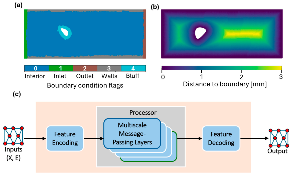
The proposed geometry-aware multiscale graph neural network (GAMS-GNN) differs from existing GNN-based CFD surrogates in several important ways. Firstly, rather than relying primarily on mesh connectivity and spatial coordinates, the framework explicitly incorporates geometry-aware information through boundary classification indicators and signed-distance-to-wall features, allowing the network to directly encode geometric proximity effects that strongly influence near-wall transport phenomena. Secondly, the proposed architecture employs a multiscale message-passing strategy that facilitates information exchange across both local and global flow regions, enabling the simultaneous representation of boundary layer physics, wake interactions, and large-scale flow structures. Thirdly, unlike many existing studies that focus on a limited set of canonical geometries, the present framework is designed to generalize across a broad family of arbitrarily shaped spline-based pin-fin geometries generated through an automated data generation pipeline. Consequently, the novelty of the proposed approach lies not solely in its application to pin-fin flows, but in the integration of geometry-aware feature encoding, multiscale graph learning, and automated geometry generalization within a unified CFD surrogate modeling framework.

To bridge this gap, the present study introduced geometry-aware multiscale graph neural network (GAMS-GNN)-based soft computing techniques, which explicitly integrated boundary-aware node and edge features, employed multiscale hierarchical message passing, and provided an adaptive framework designed specifically to resolve boundary-driven flow phenomena and generalize effectively across diverse geometries. Two-dimensional pin-fins were selected as the domain of choice—pin-fin arrays are ubiquitous in gas turbine blade cooling passages and thermal management hardware; hence, accelerating design space exploration translates directly into shorter design cycle times and rapid convergence of optimization frameworks. Additionally, these geometries involve complex flow features such as boundary layer separation, wake interactions, and stagnation zones, making them an ideal benchmark for evaluating the ability of surrogate models to capture multiscale physics.

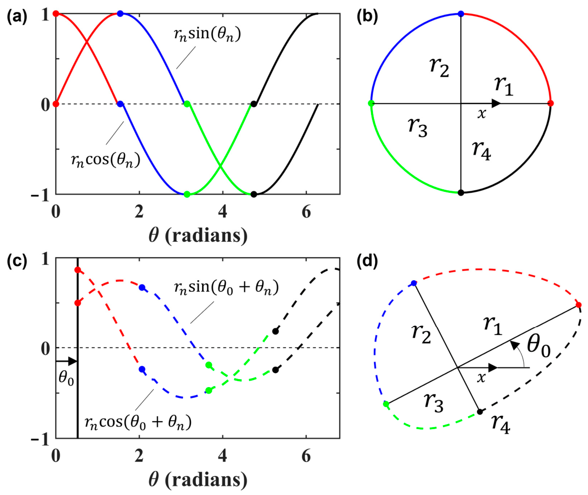
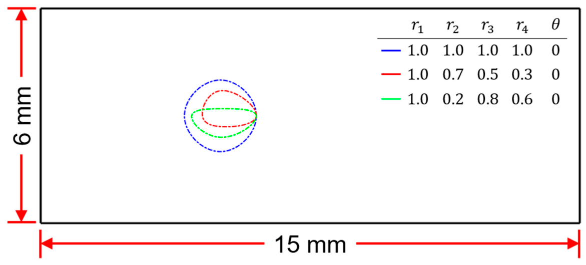
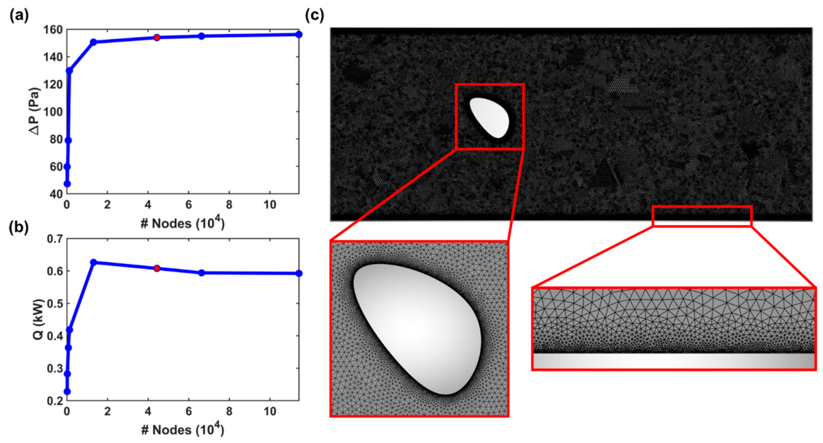
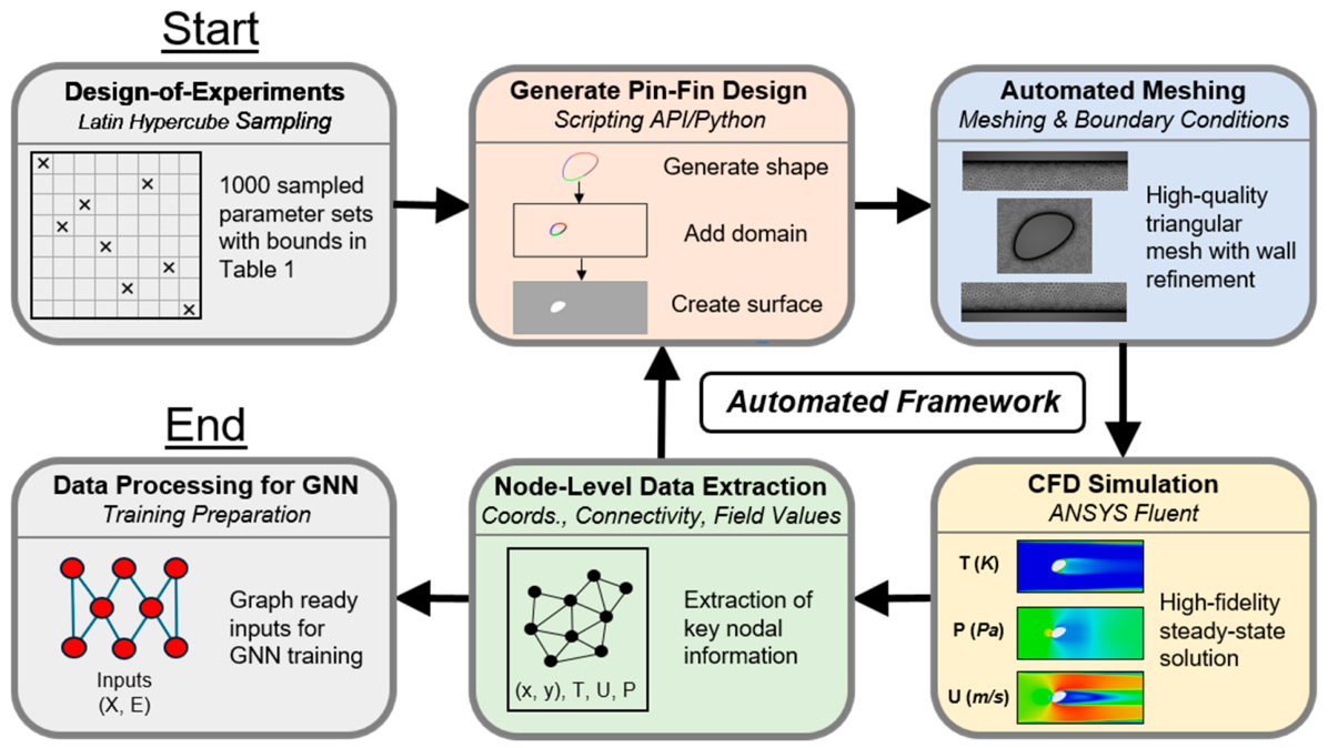
To begin with, complex pin-fin geometries were parameterized using four connecting piecewise cubic splines, providing control over the shape and orientation. The training data were generated through an automated Design-of-Experiments (DoE) framework utilizing ANSYS Fluent, incorporating best practices such as mesh refinement and validated viscous modeling. The automated framework extracted key information such as the mesh connectivity and associated field quantities to be used for training in predicting the temperature, velocity magnitude, and pressure fields. The predictive performance of GAMS-GNN was rigorously evaluated and compared against popular state-of-the-art models such as GCN [29,30] and GraphSAGE [31]. The results demonstrated that the developed GAMS-GNN achieved substantial acceleration over traditional CFD solvers but also surpassed existing SciML approaches in the accuracy, robustness, and generalization of new designs.

The remainder of the manuscript is structured as follows: Section 2 discusses the simulation methodology, data generation, GAMS-GNN model development, and data preprocessing. The observations and ensuing discussion are delineated in Section 3, while Section 4 summarizes the conclusions observed.

2. Methods

This section begins with the methodology for generating arbitrarily shaped pin-fins, followed by a detailed description of the computational domain. Subsequently, the procedures used to produce ground truth simulation data are outlined. Finally, the development and design of the GNN models are presented.

2.1. Generation of Complex Pin-Fin Shapes

The pin-fin was constructed using four connecting spline segments, each defined within a partitioned angular domain [32]. To achieve this, the angular positions of the spline endpoints were first determined by discretizing a full revolution (2π) into four equal partitions, resulting in a vector of angles, ${\theta }_n$, where ${\theta }_n=2\pi /4n$ for n = 0, 1, 2, 3. To introduce rotational flexibility, a global rotation angle, ${\theta }_0$, was added to each ${\theta }_n$, producing the final set of angular positions that defined the shape’s orientation. The radial coordinates at each of these angular positions were specified by a vector $r_n=[r_1,r_2,r_3,r_4]$, where each $r_n$ represented the radial distance from the center to the shape’s boundary at the corresponding ${\theta }_n$. These four control points—each defined by ($r_n,{\theta }_n+{\theta }_0$) in polar coordinates—served as the basis for constructing the shape using spline interpolation, ensuring a smooth transition between adjacent segments. This formulation allowed for a compact, parametric representation of the shape while maintaining control over both its geometric proportions and its orientation within the domain. The individual parametric functions $r_{n}cos\left({\theta }_n\right)$ and $r_{n}sin\left({\theta }_n\right)$, which define the boundary in Cartesian coordinates, are shown in Figure 1a. The resulting closed shape, obtained by interpolating between the control points with splines, is depicted in Figure 1b–d, illustrating a second shape generated using the same framework, but with a different set of $r_n$ values and a modified rotation angle, ${\theta }_0$, demonstrating the flexibility of the parametric design. The individual parameters and their respective bounds used in this formulation are listed in

Table 1. Geometric input parameters and bounds for pin-fin shape generation.

Parameter	Description	Bounds
$r_1$ (mm)	Radius length at $r_1$	1
$r_2$ to $r_4$ (mm)	Radius length at $r_2$ to $r_4$	[0.1, 1]
${\theta }_0$ (radians)	Orientation angle	[0, $\pi$]

. It is important to note that $r_1$ remained fixed at a constant value for all combinations to avoid mathematical errors in the spline generation.

2.2. Description of the Two-Dimensional Domain

This study investigated fluid flow and heat transfer behavior within a two-dimensional channel geometry measuring 15 mm in length (L) and 6 mm in width (W). A single pin-fin structure was introduced into the flow domain to explore its influence on local flow dynamics and thermal performance. The nominal position of the pin-fin was fixed at 5 mm downstream from the channel inlet, aligned along the channel’s centerline to ensure symmetric boundary conditions and flow development under idealized circumstances.

However, the pin-fins analyzed in this study were not limited to a single geometry; instead, they were generated using a shape generation framework designed to explore a wide morphological space. As a result of this generative process, many of the resulting pin-fin geometries were asymmetric in shape, which often caused slight shifts in their effective center of mass or spatial footprint within the channel. This led to deviations from the originally intended central location, introducing geometric variability that more accurately reflects practical design irregularities or intentionally perturbed designs.

Figure 2 provides a schematic of the overall domain, illustrating the nominal flow path and pin-fin placement. The inset table within the figure shows several examples of the generated pin-fin geometries, along with the corresponding parametric inputs (in mm) used to define their shapes. This dataset of diverse pin-fin configurations enables a broad exploration of how geometric features—such as asymmetry, elongation, and surface curvature—influence flow structures and heat transfer performance within a constrained channel.

2.3. Development of a Computational Model

2.3.1. Governing Equations and Boundary Conditions

The flow and thermal fields within the two-dimensional domain were governed by the steady-state Reynolds-Averaged Navier–Stokes (RANS) equations, which model the conservation of mass (continuity), momentum, and energy for turbulent flows. The continuity equation ensured mass conservation throughout the domain. The momentum equations accounted for the balance of forces, including pressure gradients, viscous stresses, and Reynolds stresses arising from turbulence. The energy equation described the transport of thermal energy, incorporating conduction and convective heat transfer, with the effective thermal properties adjusted to capture turbulence effects. To simplify the problem and improve computational efficiency while retaining physical accuracy, several assumptions were made: the flow was steady and two-dimensional; air was treated as the working fluid with constant thermophysical properties evaluated at 300 K; no-slip boundary conditions were applied at solid surfaces including the pin-fins and walls; and gravitational and radiative heat transfer effects were neglected.

Continuity equation:

$${\displaystyle \frac{\partial {\overline{\mathit{u}}}_{\mathit{m}}}{\partial {\mathit{x}}_{\mathit{m}}}},$$

(1)

where ${\overline{\mathit{u}}}_{\mathit{m}}$ represents the mean velocity component in the ${\mathit{x}}_{\mathit{m}}$ direction.

Momentum equation:

$$\mathsf{\rho }{\overline{\mathit{u}}}_{\mathit{n}}{\displaystyle \frac{\partial {\overline{\mathit{u}}}_{\mathit{m}}}{\partial {\mathit{x}}_{\mathit{n}}}}={\displaystyle \frac{\partial }{\partial {\mathit{x}}_{\mathit{n}}}}\left[-\overline{\mathit{P}}{\mathsf{\delta }}_{\mathit{m}\mathit{n}}+\mathsf{\mu }\left({\displaystyle \frac{\partial {\overline{\mathit{u}}}_{\mathit{m}}}{\partial {\mathit{x}}_{\mathit{n}}}}+{\displaystyle \frac{\partial {\overline{\mathit{u}}}_{\mathit{n}}}{\partial {\mathit{x}}_{\mathit{m}}}}\right)-\mathsf{\rho }\overline{{\mathit{u}}_{\mathit{m}}^{\prime }{\mathit{u}}_{\mathit{n}}^{\prime }}\right],$$

(2)

where $\mathsf{\rho }$ is the fluid density, ${\overline{\mathit{u}}}_{\mathit{n}}$ and ${\overline{\mathit{u}}}_{\mathit{m}}$ are the mean velocity components, $\overline{\mathit{P}}$ is the mean static pressure, ${\mathsf{\delta }}_{\mathit{m}\mathit{n}}$ is the Kronecker delta, $\mathsf{\mu }$ the dynamic viscosity, and $\mathsf{\rho }\overline{{\mathit{u}}_{\mathit{m}}^{\prime }{\mathit{u}}_{\mathit{n}}^{\prime }}$ the Reynolds stress representing the apparent stress due to turbulent velocity fluctuations.

Energy equation:

$${\displaystyle \frac{\partial }{\partial {\mathit{x}}_{\mathit{n}}}}\left[{\mathit{u}}_{\mathit{n}}\left(\mathsf{\rho }\mathit{E}+\mathit{P}\right)\right]={\displaystyle \frac{\partial }{\partial {\mathit{x}}_{\mathit{m}}}}\left[{\mathit{k}}_{\mathit{e}\mathit{f}\mathit{f}}{\displaystyle \frac{\partial \mathit{T}}{\partial {\mathit{x}}_{\mathit{m}}}}+{\left({\mathsf{\tau }}_{\mathit{m}\mathit{n}}\right)}_{\mathit{e}\mathit{f}\mathit{f}}{\mathit{u}}_{\mathit{m}}\right],$$

(3)

where E is the effective thermal conductivity (including molecular and turbulent contributions), T is the mean temperature, and ${\left({\mathsf{\tau }}_{\mathit{m}\mathit{n}}\right)}_{\mathit{e}\mathit{f}\mathit{f}}$ is the effective stress tensor (including both viscous and turbulent contributions), defined as follows:

$${\left({\mathsf{\tau }}_{\mathit{m}\mathit{n}}\right)}_{\mathit{e}\mathit{f}\mathit{f}}=\mathsf{\mu }\left({\displaystyle \frac{\partial {\overline{\mathit{u}}}_{\mathit{m}}}{\partial {\mathit{x}}_{\mathit{n}}}}+{\displaystyle \frac{\partial {\overline{\mathit{u}}}_{\mathit{n}}}{\partial {\mathit{x}}_{\mathit{m}}}}\right)-\mathsf{\rho }\overline{{\mathit{u}}_{\mathit{m}}^{\prime }{\mathit{u}}_{\mathit{n}}^{\prime }},$$

(4)

For the two-dimensional domain, velocity-inlet and pressure-outlet boundary conditions were imposed. The flow regime corresponded to a Reynolds number of ~10,000, with an inlet air temperature of 300 K, calculated using the two-dimensional hydraulic diameter, Dh. The outlet was maintained at a gauge pressure of zero, representing air exhausting into the ambient environment. The side walls and pin-fin were subjected to a no-slip condition and held at a constant isothermal temperature of 350 K. The inlet region was extended upstream of the pin-fin to ensure uniform flow upon initial contact. Similarly, the outlet region was extended downstream to capture the wake region and allow for flow stabilization before leaving the domain, minimizing numerical errors. A schematic representation of the boundary conditions is shown in Figure 3 with detailed specifications listed in

Table 2. Detailed specifications of domain boundary conditions in ANSYS Fluent.

Boundary	Boundary Conditions	Values
Inlet	Constant velocity	15.51 m/s
	Turbulent intensity	5%
	Hydraulic diameter	0.012 m
	Thermal	300 K
Outlet	Pressure outlet	Zero-gauge pressure
	Turbulent intensity	5%
	Hydraulic diameter	0.012 m
	Thermal	300 K
Pin-fin	No-slip—stationary wall	-
	Isothermal	350 K
Side walls	No-slip—stationary wall	-
	Isothermal	350 K

.

2.3.2. Meshing and Turbulence Model

In this study, ANSYS Fluent 2024 R2 (Ansys Inc., Canonsburg, PA, USA) was used to generate a triangular mesh with linear-order elements for the two-dimensional domain. The overall mesh element size was set to 0.05 mm, with refinement applied at the pin-fin and side walls, where the element size was reduced to 0.005 mm. This meshing strategy ensured accurate resolution of the boundary layer and thermal gradients around the pin-fin, which were critical for reliable flow and heat transfer predictions. The refined mesh near the pin-fin captured the detailed flow behavior, while the coarser mesh in the far-field regions balanced computational efficiency. To ensure the robustness of the numerical results, a grid independence study was conducted by systematically decreasing the overall element size and increasing the level of refinement at the walls, which correspondingly increased the node count.

The resulting trends in heat transfer (Q) and pressure drop (ΔP) are shown in Figure 4a and Figure 4b, respectively, as functions of the total number of nodes. Beyond the selected mesh, identified by a red dot in both plots, changes in these quantities were less than 2%, indicating convergence of the solution and validating the mesh choice used throughout this study. A representative sample mesh is shown in Figure 4c, illustrating the entire computational domain and the local refinements around an arbitrarily selected pin-fin shape. The final mesh consisted of approximately 42,000 nodes and 83,000 elements; however, with each new design, the number of nodes and elements varied based on the pin-fin shape. The SST k-ω turbulence model was employed due to its proven accuracy in resolving near-wall effects and handling adverse pressure gradients [33]. With the selected mesh resolution, the average Y+ at the pin-fin and walls was approximately 0.12, ensuring that the first cell remained well within the viscous sublayer for accurate turbulence modeling, with all values not exceeding 1 [34,35].

This mesh configuration resulted in an average simulation completion time of approximately 8 min using a system equipped with an Intel Xeon 5217 CPU, RTX 4000 GPU, and 192 GB of memory. These simulations provided the ground truth data essential for training the GNN model, capturing the critical flow and thermal characteristics necessary for robust model performance.

2.4. Dataset Generation for Training

The training dataset was generated using an enhanced version of an automated workflow [32,36], which integrates multiple software tools. Each pin-fin shape was parameterized by the geometric input variables and bounds listed in Table 1. While ${\mathit{r}}_1$ was an input parameter, it was fixed at 1 mm across all designs to prevent numerical errors in the shape generation and was therefore not included as a varying parameter. The design space was explored using a Latin Hypercube Sampling (LHS) approach to generate 1000 unique pin-fin geometries, ensuring a diverse and well-distributed dataset. An automated pipeline linked key processes, enabling seamless geometry generation, meshing, and CFD solution evaluation using ANSYS Fluent. This iterative process produced simulation results that accurately captured the flow and thermal characteristics of the system. From the mesh, individual node coordinates and connectivity were extracted, along with solution data, including temperature, pressure, and velocity values at each node location. A schematic of the automated pipeline used to generate the training data is shown in Figure 5.

2.5. Development of the Graph Neural Network (GNN) Model

2.5.1. Graph Construction and Featurization

Each CFD simulation was converted into a graph-based representation suitable for processing by a multiscale GNN. Each finite-volume cell center in the CFD mesh became a node $v_i\in V$, located at physical coordinates $x_i=(x_i,y_i)$. Edges connected nodes whose corresponding cells shared a common face, preserving the original mesh connectivity. To ensure symmetric message passing, edges were recorded bidirectionally. A typical graph contains approximately $4.23\times {10}^4$ nodes and $1.25\times {10}^5$ edges, with moderate variation across the dataset of 1000 graphs.

Each node ${\mathit{v}}_{\mathit{i}}$ carried a nine-dimensional feature vector ${\mathit{h}}_{\mathit{i}}$, which included spatial coordinates (${\mathit{x}}_{\mathit{i}}$, ${\mathit{y}}_{\mathit{i}}$), a normalized streamwise coordinate $\widetilde{{\mathit{x}}_{\mathit{i}}}$, a one-hot boundary encoding, and a signed distance to the nearest boundary. The streamwise coordinate was computed per graph as follows:

$$\widetilde{{\mathit{x}}_{\mathit{i}}}={\displaystyle \frac{{\mathit{x}}_{\mathit{i}}-{\mathit{x}}_{\mathit{m}\mathit{i}\mathit{n}}}{{\mathit{x}}_{\mathit{m}\mathit{a}\mathit{x}}-{\mathit{x}}_{\mathit{m}\mathit{i}\mathit{n}}}}$$

(5)

providing an explicit representation of flow progression from inlet $(\widetilde{{\mathit{x}}_{\mathit{i}}}=0)$ to outlet ($\widetilde{{\mathit{x}}_{\mathit{i}}}=1$). Boundary conditions were encoded using a five-dimensional one-hot vector indicating whether a node belonged to the interior fluid (0), inlet (1), outlet (2), wall (3), or bluff body surface (4), as illustrated in Figure 6a. The signed distance ${\mathit{d}}_{\mathit{i}}$ was computed as the Euclidean distance to the closest boundary point (Figure 6b). Also, each directed edge ${\mathit{e}}_{\mathit{i}\mathit{j}}$ carried a four-dimensional feature vector ${\mathit{g}}_{\mathit{i}\mathit{j}}$, defined as follows:

$${\mathit{g}}_{\mathit{i}\mathit{j}}=[\mathsf{\Delta }{\mathit{x}}_{\mathit{i}\mathit{j}},\mathsf{\Delta }{\mathit{y}}_{\mathit{i}\mathit{j}},\Vert \mathsf{\Delta }{\mathit{x}}_{\mathit{i}\mathit{j}}{\Vert }_2,\mathit{s}\mathit{i}\mathit{g}\mathit{n}\left(\mathsf{\Delta }{\mathit{x}}_{\mathit{i}\mathit{j}}\right){]}^{\mathit{T}}, \mathsf{\Delta }{\mathit{x}}_{\mathit{i}\mathit{j}}={\mathit{x}}_{\mathit{j}}-{\mathit{x}}_{\mathit{i}}$$

(6)

The first two components, $\mathsf{\Delta }{\mathit{x}}_{\mathit{i}\mathit{j}}$ and $\mathsf{\Delta }{\mathit{y}}_{\mathit{i}\mathit{j}}$, represent the relative spatial displacement between nodes and encode geometric orientation. The third component, $\Vert \mathsf{\Delta }{\mathit{x}}_{\mathit{i}\mathit{j}}{\Vert }_2$, captures the Euclidean distance between nodes, which provides a local-length scale for multiscale filtering. The final component, sign ($\mathsf{\Delta }{\mathit{x}}_{\mathit{i}\mathit{j}}$), indicates whether the edge points downstream or upstream with respect to the flow direction, introducing explicit flow alignment into the message-passing process. To ensure stable learning across the dataset, the geometric features (${\mathit{x}}_{\mathit{i}},{\mathit{y}}_{\mathit{i}},{\mathit{d}}_{\mathit{i}}$) were normalized using global z-score normalization:

$${\mathit{x}}_{\mathit{i}}^{\ast }={\displaystyle \frac{{\mathit{x}}_{\mathit{i}}-\overline{\mathit{x}}}{{\mathsf{\sigma }}_{\mathit{x}}}}, {\mathit{y}}_{\mathit{i}}^{\ast }={\displaystyle \frac{{\mathit{y}}_{\mathit{i}}-\overline{\mathit{y}}}{{\mathsf{\sigma }}_{\mathit{y}}}}, {\mathit{d}}_{\mathit{i}}^{\ast }={\displaystyle \frac{{\mathit{d}}_{\mathit{i}}-\overline{\mathit{d}}}{\mathit{d}}}$$

(7)

Here, $\overline{\mathit{x}}$, $\overline{\mathit{y}}$, and $\overline{\mathit{d}}$ are the global means of ${\mathit{x}}_{\mathit{i}}$, ${\mathit{y}}_{\mathit{i}}$, and ${\mathit{d}}_{\mathit{i}}$, respectively, while ${\mathsf{\sigma }}_{\mathit{x}}$, ${\mathsf{\sigma }}_{\mathit{y}}$, and ${\mathsf{\sigma }}_{\mathit{d}}$ are their respective standard deviations. The normalized coordinates (${\mathit{x}}_{\mathit{i}}^{\ast }$, ${\mathit{y}}_{\mathit{i}}^{\ast }$, ${\mathit{d}}_{\mathit{i}}^{\ast }$) replaced the original values in the node features, while the per-graph streamwise coordinate ${\tilde{\mathit{x}}}_{\mathit{i}}$ and one-hot encodings remained unchanged. The target variables for each node were the steady-state values of temperature ${\mathit{T}}_{\mathit{i}}$, pressure ${\mathit{P}}_{\mathit{i}}$, and velocity magnitude ${\mathit{U}}_{\mathit{i}}$, obtained from the CFD solution. These target values were normalized using global z-score statistics as well, with $\overline{\mathit{T}}$ and ${\mathsf{\sigma }}_{\mathit{T}}$, $\overline{\mathit{P}}$ and ${\mathsf{\sigma }}_{\mathit{P}}$, and $\overline{\mathit{U}}$ and ${\mathsf{\sigma }}_{\mathit{U}}$ representing the global means and standard deviations for T, P, and U, respectively:

$${\mathit{T}}_{\mathit{i}}^{\ast }={\displaystyle \frac{{\mathit{T}}_{\mathit{i}}-\overline{\mathit{T}}}{{\mathsf{\sigma }}_{\mathit{T}}}}, {\mathit{P}}_{\mathit{i}}^{\ast }={\displaystyle \frac{{\mathit{P}}_{\mathit{i}}-\overline{\mathit{P}}}{{\mathsf{\sigma }}_{\mathit{P}}}}, {\mathit{U}}_{\mathit{i}}^{\ast }={\displaystyle \frac{{\mathit{U}}_{\mathit{i}}-\overline{\mathit{U}}}{{\mathsf{\sigma }}_{\mathit{U}}}}$$

(8)

The GNN learned to predict these normalized target values directly from the input graph features. Formally, the network approximated a mapping:

$${\mathit{f}}_{\mathsf{\theta }}:\left({\mathit{h}}_{\mathit{i}},{\mathit{g}}_{\mathit{i}\mathit{j}}\right)\mapsto \left({\mathit{T}}_{\mathit{i}}^{\ast },{\mathit{P}}_{\mathit{i}}^{\ast },{\mathit{U}}_{\mathit{i}}^{\ast }\right)$$

(9)

Here, θ denotes the trainable parameters. The model was trained by minimizing the mean-squared-error (MSE) loss:

$$\mathcal{L}\left(\mathsf{\theta }\right)={\displaystyle \frac{1}{\left|\mathcal{V}\right|}}{\sum }_{\mathit{i}\in \mathcal{V}}\left[{\left({\mathit{T}}_{\mathit{i}}^{\ast }-\widehat{{\mathit{T}}_{\mathit{i}}^{\ast }}\right)}^2+{\left({\mathit{P}}_{\mathit{i}}^{\ast }-\widehat{{\mathit{P}}_{\mathit{i}}^{\ast }}\right)}^2+{\left({\mathit{U}}_{\mathit{i}}^{\ast }-\widehat{{\mathit{U}}_{\mathit{i}}^{\ast }}\right)}^2\right]$$

(10)

Here, $\widehat{{\mathit{T}}_{\mathit{i}}^{\ast }}$, $\widehat{{\mathit{P}}_{\mathit{i}}^{\ast }}$, and $\widehat{{\mathit{U}}_{\mathit{i}}^{\ast }}$ denote the network’s predicted values at each node. The dataset was randomly divided into training (70%), validation (15%), and test (15%) sets, ensuring that all subsets were representative of the full range of pin-fin geometries and mesh resolutions. Normalization parameters were stored alongside each graph and applied consistently during training and inference.

2.5.2. Model Architecture

The model followed a three-stage architecture comprising feature encoding, a processor block made of several multiscale message-passing (MMP) layers, and a final decoding module (Figure 6c). The input node features ${\mathit{h}}_{\mathit{i}}$ and edge features ${\mathit{g}}_{\mathit{i}\mathit{j}}$ were first independently projected into a shared 128-dimensional latent space using two separate multi-layer perceptrons (MLPs), denoted by ${\mathsf{\varphi }}_{\mathrm{node}}$ and ${\mathsf{\varphi }}_{\mathrm{edge}}$, respectively:

$${\mathit{h}}_{\mathit{i}}^{\left(0\right)}={\mathsf{\varphi }}_{\mathrm{node}}\left({\mathit{h}}_{\mathit{i}}\right), {\mathit{e}}_{\mathit{i}\mathit{j}}^{\left(0\right)}={\mathsf{\varphi }}_{\mathrm{edge}}\left({\mathit{g}}_{\mathit{i}\mathit{j}}\right)$$

(11)

The encoded graph was then passed through a stack of four multiscale message-passing (MMP) layers, each operating over a multiresolution graph hierarchy. Within each MMP layer, message passing was performed at several coarsened levels using seven sequential message-passing layer blocks. Each of these blocks updated both edge and node features via MLPs:

$${\mathit{e}}_{\mathit{i}\mathit{j}}^{\left(\mathit{l}\right)}\leftarrow {\mathit{e}}_{\mathit{i}\mathit{j}}^{\left(\mathit{l}-1\right)}+{\mathsf{\varphi }}_{\mathrm{edge}}^{\left(\mathit{l}\right)}\left(\left[{\mathit{h}}_{\mathit{i}}^{\left(\mathit{l}-1\right)},{\mathit{h}}_{\mathit{j}}^{\left(\mathit{l}-1\right)},{\mathit{e}}_{\mathit{i}\mathit{j}}^{\left(\mathit{l}-1\right)}\right]\right)$$

(12)

$${\mathit{h}}_{\mathit{i}}^{\left(\mathit{l}\right)}\leftarrow {\mathit{h}}_{\mathit{i}}^{\left(\mathit{l}-1\right)}+{\mathsf{\varphi }}_{\mathrm{node}}^{\left(\mathit{l}\right)}\left(\left[{\mathit{h}}_{\mathit{i}}^{\left(\mathit{l}-1\right)},{\sum }_{\mathit{j}\in \mathcal{N}\left(\mathit{i}\right)}{\mathit{e}}_{\mathit{i}\mathit{j}}^{\left(\mathit{l}\right)}\right]\right)$$

(13)

Here, the edge update depends on both the incoming node embeddings and existing edge features, while the node update aggregates neighborhood edge messages and combines them with the current node state. Both update steps incorporated ReLU activation and layer normalization. Each MMP layer performed hierarchical pooling and unpooling across multiple graph resolutions. The graph was coarsened using voxel-based spatial binning with resolution controlled by a characteristic edge length. After downward passes through increasingly coarse graphs, node features were interpolated back to finer graphs using k-nearest neighbor interpolation (with k = 4), followed by upward message passing to refine the representations. The final output was produced by another MLP decoder ${\mathsf{\varphi }}_{\mathrm{decode}}$, which mapped the latent node embeddings ${\mathit{h}}_{\mathit{i}}^{\mathrm{fnl}}$ to the predicted physical fields:

$$\left(\widehat{{\mathit{T}}_{\mathit{i}}^{\ast }},\widehat{{\mathit{P}}_{\mathit{i}}^{\ast }},\widehat{{\mathit{U}}_{\mathit{i}}^{\ast }}\right)={\mathsf{\varphi }}_{\mathrm{decode}}\left({\mathit{h}}_{\mathit{i}}^{\mathrm{fnl}}\right)$$

(14)

Here, $\widehat{{\mathit{T}}_{\mathit{i}}^{\ast }}$, $\widehat{{\mathit{P}}_{\mathit{i}}^{\ast }}$, and $\widehat{{\mathit{U}}_{\mathit{i}}^{\ast }}$ are the predicted temperature, pressure, and velocity magnitude, respectively, at node i. This formulation enabled the model to efficiently aggregate both local and global flow features across nonuniform CFD domains. All updates—including edge and node updates—were performed entirely using learnable MLPs rather than fixed convolutional filters, making the architecture highly expressive and adaptable to mesh-based variations across samples.

All training was performed on a single NVIDIA Tesla V100 GPU hosted on the Roar Collab high-performance computing cluster at the Institute for Computational and Data Sciences, the Pennsylvania State University, University Park, PA, USA. The network was optimized with the Adam optimizer (initial learning rate 2 × 10⁻⁴, with a decay of 0.5 every 25 epochs). Training for 100 epochs on the 700-graph dataset required a wall time of around 6 h. Inference was performed on the dual-processor Intel^® Xeon^® Gold 6230R CPU, (Round Rock, TX, USA) operating at a base frequency of 2.1 GHz. The inference time was clocked at less than 1 s for a single graph, ~500 times the speedup compared to that of the Fluent RANS solver.

3. Results and Discussion

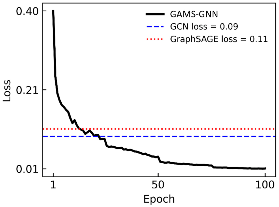
The training loss trajectory of the GAMS-GNN is shown in Figure 7, alongside horizontal reference lines that mark the terminal losses of the naive GCN and GraphSAGE baselines. GAMS-GNN achieved an MSE of ≈ 0.01, while the baselines stabilized at substantially higher values—0.11 for GraphSAGE and 0.09 for GCN—an order-of-magnitude performance gap in favor of GAMS GNN. Although the proposed network contained 11.6 million trainable parameters, roughly 15× more than the 0.79 million in each baseline, this additional capacity was well utilized: the edge-aware, multiscale architecture delivered markedly richer representations rather than over-fitting, translating directly into superior predictive accuracy.

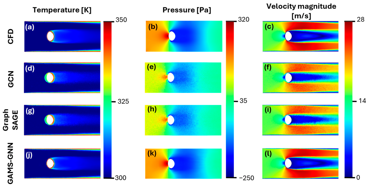
Figure 8 presents a side-by-side comparison of the temperature, pressure, and velocity magnitude fields predicted by the three graph surrogates against the CFD ground truth. The first row, Figure 8a–c, shows the reference CFD solution: sharp thermal gradients following the contours of the fin surface, a well-defined high-pressure velocity stagnation region on the upstream face, and a coherent recirculation region with accelerated side channel jets downstream. In the second and third rows, the naïve baselines—GCN in Figure 8d–f and GraphSAGE in Figure 8g–i—captured only the broad trends: temperature contours were blurred, the stagnation pressure pocket was diffuse, the wake velocity was oversmoothed, and boundary layer separation was delayed, with noticeable artifacts in the pressure field. The fourth row, GAMS-GNN in Figure 8j–l, recovered the fine-scale details evident in the CFD: the near-wall thermal boundary layer heating in Figure 8j, the well-defined, highly resolved, and precisely captured high-to-low-pressure transition in Figure 8k, and the recirculation zone and shear layer jets in Figure 8l aligned closely with their counterparts in Figure 8a–c. By preserving sharp gradients and eliminating baseline noise, GAMS-GNN demonstrates its capability to reproduce boundary-driven, multiscale phenomena—qualitative evidence that supports the order-of-magnitude error reduction seen in the convergence plot shown in Figure 7.

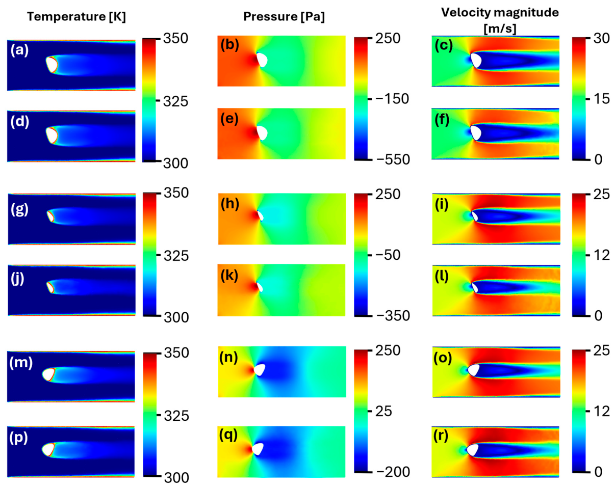
Figure 9 juxtaposes the ground truth CFD solutions with GAMS-GNN predictions for three geometrically distinct arbitrary pin-fin configurations from the test dataset. In the first set, panels Figure 9a–c exhibit the reference temperature, pressure and velocity fields for the first pin-fin, while panels Figure 9d–f display the corresponding GAMS-GNN outputs. The agreement is essentially pointwise: the network preserved the narrow thermal rim that formed along the upstream face, reproduced both the magnitude and spatial extent of the upstream high-pressure stagnation pocket, and captured the length and width of the recirculation zone together with its accelerated side channel jets. This first pin-fin resembled several members of the training ensemble in aspect ratio and blockage ratio, and the model’s edge-aware encoder retained the steep boundary layer gradients that characterize such fins; multiscale message-passing then disseminated this information throughout the short wake, leaving negligible room for perceptible error.

The second arbitrary pin-fin, depicted in panels Figure 9g–i for the CFD reference and Figure 9j–l for GAMS-GNN, posed a sterner test. A sharper nose and higher blockage ratio yielded a shorter, narrower wake in the CFD solution. While the network continued to track temperature and upstream pressure with high fidelity, it underpredicted the downstream momentum deficit: the low-velocity core in panel Figure 9l is shorter and narrower than its counterpart in panel Figure 9i, and the pressure dip in panel Figure 9k recovers slightly too quickly. These discrepancies arise from two interacting factors. Firstly, the loss function weighed all nodes equally; because the recirculation zone occupied a small fraction of the domain, its contribution to the global error budget was limited, encouraging the optimizer to privilege more extensive, lower-gradient regions. Secondly, the effective receptive field of the graph, although enlarged by hierarchical message passing, still contracted with distance from the fin, so far wake nodes received attenuated information about earlier separation and recirculation patterns.

Panels Figure 9m–r present the third fin, a bluff front design that accentuated leading-edge gradients and narrowed the shear layer. GAMS-GNN accurately reproduced the intensified boundary layer heating, matched peak wall temperatures, and resolved the sharper stagnation pressure transition. The predicted velocity field mirrored the CFD recirculation region and shear layer jets, indicating that the network’s skip connections successfully reinjected fine-scale information lost during coarsening.

A closer inspection of the four-spline design space clarifies why the “stubby’’ or “blunt” cross-section embodied by the second arbitrary pin-fin was so sparsely represented in the 1000-member training set, despite the use of LHS. Each profile was defined by five parameters: a fixed leading-edge radius ${\mathit{r}}_1=1 \mathrm{mm}$; three free radii r₂, r₃, and r₄ drawn independently from the interval [0.1, 1] mm; and a global orientation angle ${\mathsf{\theta }}_0$ uniformly distributed over [0, π]. 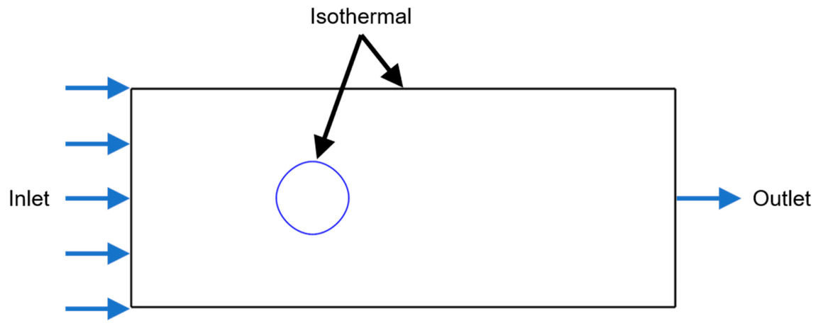Once the four polar control points (${\mathit{r}}_{\mathit{n}},{\mathsf{\theta }}_{\mathit{n}}+{\mathsf{\theta }}_0$) with ${\mathsf{\theta }}_{\mathit{n}}=\mathit{n}\hspace{0.17em}\mathit{\pi }/2(\mathit{n}=0-3)$ were set, piecewise cubic splines joined successive points, producing the closed outline shown in Figure 1.

The streamwise chord c and cross-stream width d of the resulting body are, to first order, the differences between the largest and smallest projections of the radii onto the flow axis and its perpendicular, respectively. Achieving a low chord-to-width ratio (c/d)—the defining geometric trait of the second pin-fin—demands two statistically independent coincidences. Firstly, both radii that ultimately align with the flow direction after rotation must reside in the lower third of their admissible range, compressing c. Because LHS placed each ${\mathit{r}}_{\mathit{k}}$ once in every decile, the likelihood that a particular pair of radii simultaneously fell into the lowest tertile is ${\left({\displaystyle \frac{1}{3}}\right)}^2\approx 0.11$. Secondly, the large, fixed radius ${\mathit{r}}_1$ must be rotated toward the cross-stream axis so that it inflates d. Orientations that satisfy this requirement occupied only a quarter of the ${\mathsf{\theta }}_0$ interval (±22.5° about 90° or 270°), giving a probability of 0.25. The two events are uncorrelated under LHS; therefore, the joint probability of drawing a genuinely stubby fin is the product of the two, $\approx 0.11\times 0.25=0.0275$. On average, then, fewer than thirty of the 1000 LHS samples inhabit this low-c/d corner of the five-dimensional hypercube, whereas hundreds populate the moderate- and high-ratio region typified by the first and the third fins.

This numerical imbalance carried direct consequences for learning. During training, the global mean-squared-error loss was dominated by the plentiful, moderate-slenderness sections; weight updates therefore embedded wake recovery dynamics characteristic of those shapes. When GAMS-GNN confronted a rare stubby geometry such as the second pin-fin, it reproduced near-body gradients accurately—physics that depends mainly on local curvature, which the network has seen often—but extrapolated the downstream momentum deficit from scant experience, shortening the already brief wake and hastening pressure recovery. In essence, the model behaved as an approximately Bayesian estimator whose prior was set by the frequency distribution of the training set: it had a sharp, well-informed prior for moderate-c/d fins and a diffuse, weakly informed prior for low-c/d fins, leading to underprediction of wake length in the latter.

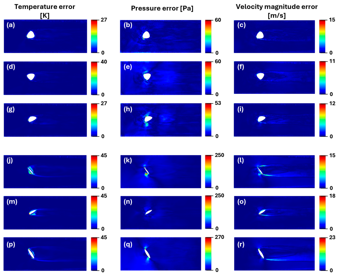
The variable-specific error maps of Figure 10 reveal how geometric features drove prediction performance. The first three rows correspond to the three best-performing fins from the testing dataset; Figure 10a–c depict the temperature error, pressure error, and velocity magnitude error, respectively, for the first fin, with the same column ordering used for the rest. Similarly, the last three rows indicate the three worst-performing fins from the test set. Interestingly, for the three best fins, the stagnation point pressure error was below 60 Pa, and the velocity magnitude error decayed rapidly as well, keeping temperature errors under 30 K throughout the wake. In contrast, all three worst-performing fins (rows 4–6) shared two features absent from most training samples: a chord-to-depth ratio (c/d < 1) and at least one acute or concave leading-edge corner. These traits triggered local pressure overshoots of 250–270 Pa—more than four times larger than in the well-represented shapes—which in turn shortened the recirculation bubble and intensified side-jet velocities. Elevated temperature errors (35–45 K) simply mirrored the misplaced convective heat paths. The pattern confirms that GAMS-GNN’s largest discrepancies stem from under-represented geometric extremes rather than intrinsic model capacity, suggesting that an active-learning loop focusing on low-c/d, high-curvature fins could systematically eliminate the remaining error hotspots.

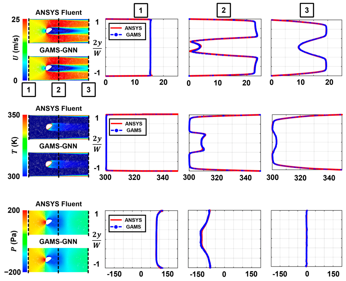
To further validate the performance of the GAMS-GNN model in capturing key fluid dynamic behavior, spanwise profiles of velocity magnitude, temperature, and pressure were extracted at three representative streamwise locations: the inlet (1), midline (2), and outlet (3) of the computational domain. These regions are critical not only for assessing flow development and evaluating thermal–hydraulic performance but also for capturing complex physical phenomena—particularly at the midline (2), where recirculation and boundary layer evolution drive much of the local flow–thermal behavior. Accurate modeling in these regions is essential, as they significantly influence key engineering metrics such as pressure drop and heat transfer, which are often derived from area-weighted averages at critical locations such as the inlet and outlet.

Figure 11 provides a comprehensive comparison of the velocity magnitude (top row), temperature (middle row), and pressure (bottom row) profiles at these streamwise locations. The respective contour plots from ANSYS Fluent and the GAMS-GNN predictions are displayed in the left-most column for each row. On these contours, a black dotted line is present to indicate the streamwise location (1—inlet, 2—midline, 3—outlet) where these field values were extracted. On the right, the spanwise profiles of the same quantities are shown, with the y-axis normalized using 2y/W, where y is the vertical coordinate, and W represents the width of the domain. This normalization ensured that the profiles were bound between −1 and 1, enhancing readability. The x-axis represents the magnitude of the respective field variable in the spanwise direction.

The temperature profiles, particularly at the inlet and outlet regions, aligned closely between the GAMS-GNN predictions and ANSYS Fluent, capturing both the thermal boundary layer development and the steady-state behavior at the outlet. The GAMS-GNN also successfully represented the temperature variation near the midline, where recirculation effects are critical in determining thermal performance. Similarly, the velocity profiles showed excellent agreement, with the GAMS-GNN successfully replicating boundary layer growth at the inlet and side walls, boundary layer separation and recirculation in the midline, and the stabilization of the flow at the outlet. The pressure profiles reflect accurate predictions for GAMS-GNN, which were consistent with ANSYS Fluent. Notably, at the inlet, where the flow initially contacts the pin-fin, GAMS-GNN captured the stagnation point and the high-pressure region that forms. In the midline, the GAMS-GNN prediction not only replicated the effects of recirculation but also captured the pressure drop associated with the presence of a bluff body, as depicted by the negative values seen in the midline pressure panel.

In all, the GAMS-GNN model proved to be a robust tool for capturing key fluid dynamic and thermal–hydraulic behavior, outperforming current approaches with unparalleled accuracy across temperature, velocity, and pressure profiles, all while significantly reducing computational time. The GAMS-GNN successfully captured the steep gradients commonly found in complex flow regimes, such as those near the boundary layers, where rapid transitions between high and low values occur. Additionally, the model excelled in handling recirculation zones, where traditional models often struggle to capture the intricate flow behavior, especially in a domain where the shapes under consideration are highly complex and irregular.

4. Conclusions

In this study, a geometry-aware multiscale (GAMS)-GNN was developed for steady, turbulent flow field prediction around complex pin-fins in a two-dimensional channel. The conclusions of this paper can be summarized as follows:

• A training dataset was generated using an automated pipeline that integrated geometry generation, high-resolution meshing, and CFD simulation solutions through ANSYS Fluent. The design space—defined by five geometric parameters—was explored using Latin Hypercube Sampling (LHS) to produce 1000 different pin-fin configurations. For each design, mesh-based node coordinates, connectivity, and flow solution variables were extracted to construct a rich dataset for training.
• Each CFD simulation was transformed into a graph, in which nodes represented finite-volume cell centers, and edges reflected mesh connectivity. Each node carried information about its spatial coordinates, a normalized streamwise position, a one-hot encoded boundary indicator, and a signed distance to the nearest wall, providing geometric and physical context. These graphs served as inputs to the GAMS-GNN, which predicted the temperature, velocity magnitude, and pressure at each node based on learned flow physics.
• The GAMS-GNN model accurately captured the steady turbulent flow–thermal behavior across the channel domain. Spanwise profiles of the temperature, velocity magnitude, and pressure closely matched results from ANSYS Fluent, successfully reproducing boundary layer development and separation, recirculation effects, and stagnation zones. The model demonstrated strong predictive performance in areas with steep gradients and complex flow patterns, validating its robustness for modeling irregular pin-fin geometries with significantly reduced computational cost.

Ultimately, GAMS-GNN demonstrated a substantial leap in predictive modeling by learning and generalizing the underlying physical behavior of complex, steady turbulent flow regimes. Its ability to accurately capture recirculation, boundary layer development, stagnation, and steep thermal and velocity gradients across highly irregular pin-fin geometries showed that the model internalized core fluid dynamics principles. This data-driven approach, without any explicit physics-based regularizations, effectively captured the same flow-defining features resolved by the RANS solver, achieving performance indistinguishable from ANSYS Fluent, which explicitly solved the underlying partial differential equations of mass, momentum, and energy conservation. As a result, GAMS-GNN offered a powerful and computationally efficient framework for advancing the design and optimization of thermal–fluid systems, especially in cases where traditional GNN models struggled to resolve geometric complexity or required prohibitively expensive simulations. To further substantiate near-wall predictive fidelity, the accuracy of wall-normal temperature gradients and the corresponding local Nusselt number distributions along the fin surfaces is acknowledged as an important direction for quantitative evaluation in future work.