Quantifying the Stability–Recovery–Interpretability Trade-Off Between K-Means and Self-Organizing Maps for High-Dimensional Imbalanced Data

Abstract

High-dimensional engineering datasets often combine class imbalance, noisy structures, and limited ground truth, making unsupervised analysis difficult to evaluate reliably. This study quantifies how three properties—partition stability, minority class recovery, and topological interpretability—are traded off across clustering methods, using a capacity-matched 25-seed comparison on a TCGA-derived RNA expression dataset (10,095 samples, 19 cancer types, 13,634 genes). We compare K-means across cluster counts $k\in \{19,\dots ,400\}$, self-organizing maps (SOMs) across lattice sizes from 25 to 625 nodes, consensus K-means, a granularity-matched SOM-Super20 control, and four modern baselines (HDBSCAN, spectral clustering, Gaussian mixtures, and Leiden). At matched prototype budgets, K-means is both more reproducible and substantially better at recovering minority classes than SOMs: at 400 prototypes, K-means achieves pairwise NMI $0.819$ versus $0.621$ for the $20\times 20$ SOM and recovers the smallest cancers 6–$14\times$ more effectively (pancreas effective coverage $0.760$ vs. $0.054$).Crucially, the SOM does not close this gap even when given more prototypes ($0.07$ at 625 nodes), so, under matched capacity, minority recovery is better explained by representational capacity and centroid allocation freedom than by topology preservation. The recovery is not free: increasing k overfragments the partition and lowers the pairwise ARI stability ($0.643\to 0.419$ from $k=20$ to $k=400$), while the NMI remains robust ($\approx 0.82$). The hardest minority, pancreas, is recovered only by high-capacity K-means and by no other method evaluated, including SOMs at any size, consensus K-means, SOM-Super20, HDBSCAN, Gaussian mixtures, spectral clustering, and Leiden. The SOM’s distinct value is therefore not stability or recovery but the interpretable two-dimensional topological visualization that it uniquely provides, including a gradient-organized structure that is reproducible across seeds for kidney (weaker for uterus). No single method optimizes all three properties; the appropriate choice depends on whether a task prioritizes reproducibility, minority recovery, or visual interpretability. Because these conclusions follow from the shape of the data and the allocation behavior of the algorithms rather than from biological semantics, we expect them to transfer to high-dimensional imbalanced engineering data, such as those from fault clustering, condition monitoring, and anomaly detection.

1. Introduction

Modern engineering increasingly relies on unsupervised machine learning to extract structures from high-dimensional, noisy, imbalanced datasets where the ground truth is partial, imperfect, or unavailable. Examples span fault clustering in industrial systems, condition monitoring in manufacturing, remote sensing land cover analysis, and biological subtype discovery from omics data. Three demands recur across these domains: partition stability—the requirement that rerunning the analysis with a different random seed should produce the same groupings; minority class recovery—the requirement that small but important classes (rare faults, rare anomalies, rare subtypes) are actually surfaced rather than absorbed into larger groups; and interpretability—the requirement that an engineer or domain expert can inspect, audit, and reason about the result. These demands are often in tension. Stability requires algorithms with few cluster prototypes and tight, well-separated decisions (e.g., K-means). Interpretability requires algorithms that preserve the geometry of the input space and expose neighborhood relationships among samples (e.g., topology-preserving methods such as self-organizing maps). Minority recovery, as we show, depends on a third axis—representational capacity and the freedom with which a method may place prototypes—that does not align cleanly with either of the other two.

This paper addresses the trade-off directly. We perform a capacity-matched, multi-seed comparison of K-means and SOMs—together with consensus K-means, a granularity-matched SOM-Super20 control, and four modern clustering baselines—on a single, realistic, imbalanced dataset: a TCGA-derived RNA expression compendium of $\mathrm{10,095}$ samples spanning 19 cancer types. By sweeping cluster cardinality for both primary methods, we separate effects that are genuinely algorithmic from effects that are merely artifacts of how many prototypes a method is allowed. Our goal is not to declare a superior method but to characterize which property—stability, minority recovery, or interpretability—each method delivers and at what cost.

1.1. Background and Prior Work in This Project

In our prior work [1], we applied K-means with recursive subclustering to the same TCGA dataset, achieving roughly $84\%$ alignment with recorded cancer type labels and observing candidate subtype-like subclusters in brain and kidney. Two limitations of this study motivated the present work.

• Stochastic instability was not quantified. Per-cancer purity and recursive refinement outcomes varied across runs without an explicit reproducibility analysis.
• Flat partitions cannot represent neighborhood structure. K-means produces partitions where “cluster 5” and “cluster 6” are arbitrarily numbered—there is no notion of cluster proximity. This structurally precludes the detection of gradient-organized variation within a cancer type or between related cancers.

The present work directly addresses both, using the same dataset and the same preprocessing but adding (i) a 25-seed stability evaluation protocol applied to both methods and (ii) a topology-preserving SOM as a second method, whose interpretability we explicitly compare to that of K-means.

1.2. Contributions

We offer five engineering-level contributions.

C1. 

A reproducible, capacity-matched evaluation pipeline for unsupervised structure discovery on imbalanced high-dimensional data: within-method stability and per-class coverage measured across cluster cardinality for K-means ($k\in \{19,20,25,50,100,200,400\}$, each at n_init$\in \{1,10,20\}$) and SOMs (lattices of 25–625 nodes), together with consensus K-means, SOM-Super20, and four modern baselines (HDBSCAN, spectral, Gaussian mixtures, Leiden), all under one 25-seed protocol on matched standardized data. All hyperparameters, trained models, and per-run metrics are released.

C2. 

A capacity-matched stability comparison showing that K-means is more reproducible than SOMs regarding both the NMI and ARI at every matched prototype budget. Because the comparison is performed at equal cardinality, the stability gap cannot be dismissed as a partition granularity artifact, strengthening rather than qualifying the aggregate finding.

C3. 

The central result: under matched capacity, minority class recovery is driven by representational capacity and centroid allocation freedom rather than by topology preservation. At a matched budget of 400 prototypes, unconstrained K-means recovers the smallest cancers 6–$14\times$ better than the lattice-constrained SOM, and the SOM fails to match it even at 625 nodes. This recovery is traded off against pairwise ARI stability (which falls from $0.643$ at $k=20$ to $0.419$ at $k=400$, while the NMI is preserved), establishing a three-way stability/recovery/interpretability trade-off that no single method resolves.

C4. 

A breadth comparison showing that recovery is strongly method- and class-specific: spectral clustering and Leiden recover testes and thymus but not pancreas; consensus K-means, SOM-Super20, HDBSCAN, and Gaussian mixtures recover none of the three; and pancreas is recovered only by high-capacity K-means. We introduce an effective coverage metric (capture rate × dominant cluster purity) to conduct these comparisons on a single bounded scale.

C5. 

The characterization of topology preservation’s contribution—interpretability rather than recovery. The SOM uniquely provides a two-dimensional topological visualization (U-matrices, hit maps, dominant label and purity maps, per-cancer density overlays) and exposes a gradient-organized structure; we quantify the seed stability of this structure and find it reproducible for kidney and seed-dependent for uterus.

1.3. Scope and Non-Goals

We deliberately limit our scope to the unsupervised structure-and-trade-off question. We do not claim the discovery of new biological cancer subtypes, do not perform external cohort validation, and do not integrate multi-omics or clinical outcome data. These are necessary follow-ups (Section 6) but lie outside the methodological focus of this paper. Although transcriptomic data are used as the experimental domain, the proposed framework is intended as a general methodology for evaluating unsupervised AI systems operating on high-dimensional, imbalanced data; we explicitly note that its transfer to engineering domains is a hypothesis grounded in the data shape and algorithmic properties that we establish, to be tested on engineering benchmarks (Section 5.5), rather than a result demonstrated here.

2. Related Work

2.1. Cancer Subtype Discovery from Expression Data

Ref. [2] established RNA sequencing as a standard tool for high-resolution transcriptomic profiling. The Cancer Genome Atlas [3] provides compendia of thousands of tumor expression profiles. Both supervised and unsupervised approaches have been applied: deep neural networks [4,5] when labels are trusted and K-means [6], hierarchical clustering, NMF, and consensus clustering frameworks [7] for exploratory discovery. A recurring observation across these studies is that subtype calls are often not stable across cohorts, methods, or random seeds [8,9], motivating frameworks that quantify rather than ignore reproducibility.

2.2. Self-Organizing Maps for High-Dimensional Data

The self-organizing map [10] is an unsupervised neural network that maps high-dimensional input vectors to a low-dimensional (typically 2D) lattice while preserving local neighborhood relationships. Standard diagnostics include the unified distance matrix (U-matrix) [11], showing inter-node distances; hit maps, showing sample density; and component planes, showing per-feature distributions across the lattice. SOMs have been applied to gene expression [12,13], climate analysis [14], and biomedical diagnostics [15]. Two practical concerns are documented: (i) the map size must balance granularity against node occupancy [16] and (ii) rectangular topologies exhibit a border effect where edge nodes absorb outliers because they have fewer competing neighbors.

2.3. Clustering Stability and Reproducibility

Clustering stability has been recognized for two decades as a necessary criterion for trustworthy unsupervised analysis [17,18]. Common quantification metrics include the NMI [19] and the Adjusted Rand Index [20]. Consensus clustering [7] aggregates multiple runs into co-assignment matrices, and bootstrap stability has been applied in medical phenotyping [21]. Despite this body of work, many recent cancer subtyping pipelines report only single-run results and do not include explicit pairwise stability evaluations against an alternative clustering method—one of the gaps that this paper addresses.

2.4. Class Imbalance in Unsupervised Learning

Class imbalance is well studied in supervised learning but receives less attention in unsupervised settings. Centroid-based methods such as K-means are known to allocate cluster centers preferentially to high-density regions, which can leave minority classes unrepresented. Topology-preserving methods allocate prototypes more uniformly across the lattice, which has been suggested to mitigate minority class neglect [22]. Quantitative head-to-head comparisons on imbalanced real data remain rare, however, and—as our capacity-matched analysis (Section 4.4) shows—this suggestion does not hold once method capacity is controlled: at a matched prototype budget, the centroid-based method recovers minorities far better than the topology-preserving one, indicating that minority recovery is governed by capacity and allocation freedom rather than by topology preservation itself.

2.5. Explainable AI in Engineering and Biomedicine

Explainability is now a recognized goal for AI applied to engineering and biomedical domains [23,24]. For unsupervised methods, explainability comprises both algorithmic transparency (the procedure must be auditable) and visual interpretability of the resulting structure (the user must be able to see and understand the partition). SOMs naturally support the second requirement through their 2D lattices. Combining SOM visualization with explicit stability quantification yields an exploratory framework that is reproducible and inspectable.

2.6. What the Existing Literature Leaves Unanswered

Although both SOM-based expression analysis and clustering stability methodologies represent mature subfields, their intersection has not been systematically examined. Most prior expression-SOM studies [12,13] evaluate the lattice qualitatively—through the visual inspection of U-matrices, hit maps, and overlays—and report results for a single trained map. Stability across initializations is rarely quantified, and head-to-head comparison against the centroid-based baseline that practitioners actually use (K-means) is rarer still. Where multi-seed evaluations do appear, they are typically single-method (SOM only or K-means only) and do not isolate the contribution of class imbalance to per-method stability profiles. To our knowledge, no prior study has combined (i) a paired multi-seed protocol applied to both SOMs and K-means under matched data and seeds, (ii) an explicit comparison against consensus K-means as the standard remedy for single-run instability, and (iii) a per-class breakdown that exposes how class imbalance interacts with each method’s prototype allocation strategy. This paper provides these three components together, yielding a quantitative picture of when each method is appropriate that is not derivable from prior single-method or single-run results.

3. Materials and Methods

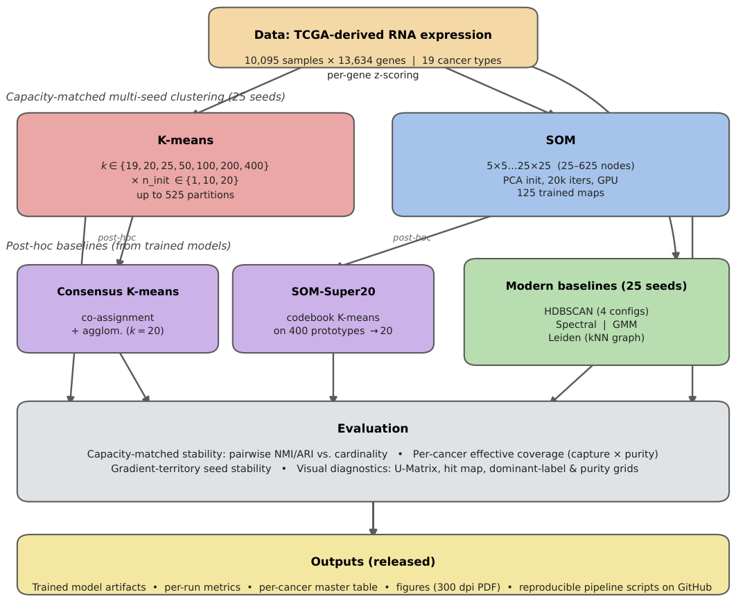
Figure 1 summarizes the experimental pipeline. We preprocess the TCGA-derived expression compendium (Section 3.1), train the two primary clustering methods across a range of cluster cardinalities over 25 random seeds (SOM at 25–625 nodes, Section 3.3; K-means at $k\in \{19,\dots ,400\}$ and n_init $\in \{1,10,20\}$, Section 3.4), derive two post hoc baselines from the SOM and K-means runs (consensus K-means, Section 3.5; SOM-Super20, Section 3.6), add four modern clustering baselines (Section 3.7), and evaluate all methods through paired stability metrics and per-cancer effective coverage (Section 3.9 and Section 3.10). The capacity sweep (Section 3.8) allows us to separate algorithmic effects from prototype budget effects.

3.1. Dataset

We use the same TCGA-derived transcriptomic compendium employed in our prior work [1]: $\mathrm{10,095}$ RNA expression samples across 19 primary cancer types, with $\mathrm{13,634}$ gene expression features per sample. The class composition is heavily imbalanced (squamous $n=1507$; thymus $n=106$; full distribution in

Table 1. Class distribution of the TCGA-derived compendium ($N=\mathrm{10,095}$), sorted by class size.

Cancer	n	Cancer	n	Cancer	n
Squamous	1507	Lung	599	Adrenal	256
Breast	1153	Thyroid	553	Leukemia	199
Kidney	974	Uterus	530	Pancreas	151
Brain	696	Prostate	525	Testes	110
Colorectal	659	Melanoma	512	Thymus	106
Liver	455	Stomach	433
Ovary	357	Sarcoma	320

). Each sample is identified by a string of the form <cancer_type>.<n> (e.g., brain.391); the cancer type prefix serves as the recorded label for evaluation only and is not used during clustering. The ∼14× class size imbalance (1507 vs. 106) is representative of typical engineering datasets and motivates the per-cancer analysis in Section 4.4.

3.2. Preprocessing

The dataset as distributed contained log-scale expression values (approximate range $-9.2$ to $+8.4$; per-gene std median $0.79$, max $4.83$), indicating a log-transformation but not full per-gene standardization. We applied per-gene z-scoring (StandardScaler from scikit-learn) so that all genes contributed on a comparable scale to Euclidean distance-based methods. After standardization, the per-gene mean $\approx 0$ and std $=1$. No additional dimensionality reduction or gene filtering was applied; the full $\mathrm{13,634}$-gene representation is used as input for all clustering methods.

3.3. Self-Organizing Map Configuration

We use the MiniSom implementation [25] of the standard Kohonen SOM [10]. The map consists of a 2D lattice of nodes, each carrying a prototype vector in the input space. During training, each input vector is assigned to its best-matching unit (BMU)—the node whose prototype is closest under Euclidean distance—and prototypes of the BMU and its lattice neighbors are updated toward the input. The neighborhood is Gaussian with a width that decays during training; the learning rate similarly decays.

3.3.1. Operating Point for Visualization

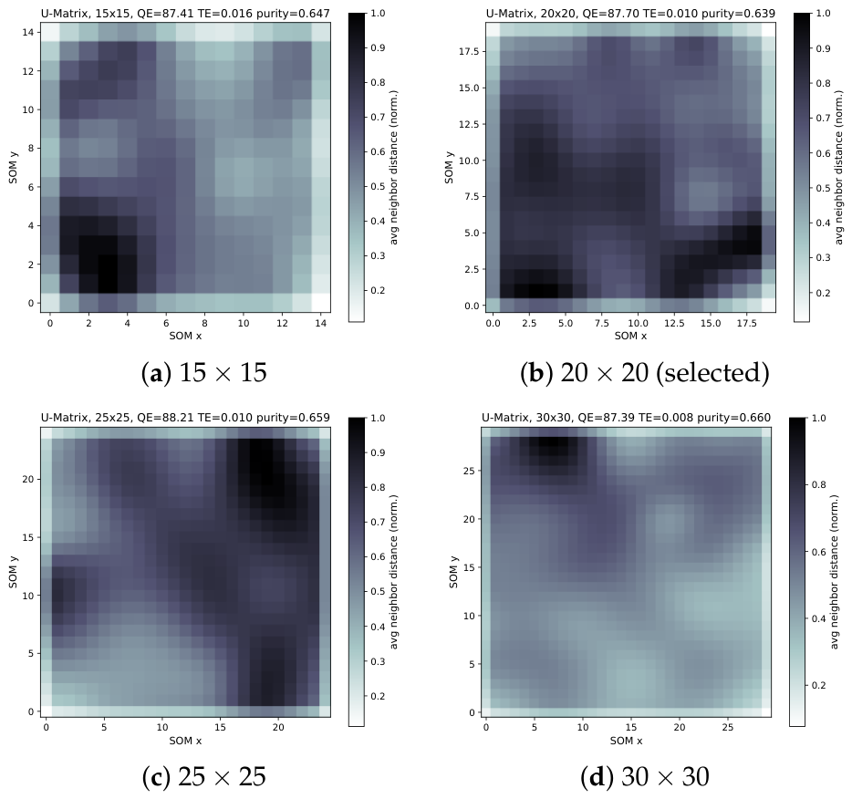
We performed a grid size sweep at $15\times 15$, $20\times 20$, $25\times 25$, and $30\times 30$ (Section 4.1). All sizes produced similar quantization errors (87.4–88.2) and topographic errors (0.008–0.016), with weighted label purity of 0.639–0.660.The $20\times 20$ lattice was selected as the visualization operating point because it balances 97% node occupancy against tractable training time; all qualitative diagnostics (Section 4.5 and Section 4.6) rely on this lattice.

3.3.2. Capacity Sweep

For the capacity-matched comparison against K-means (Section 3.8), we additionally train SOMs at $5\times 5$, $10\times 10$, $15\times 15$, $20\times 20$, and $25\times 25$ (25, 100, 225, 400, and 625 nodes), $\times 25$ seeds each (125 trained maps). These sizes were chosen so that the SOM prototype counts spanned the K-means k range, enabling a like-for-like comparison at matched cardinality ($\approx 25$, $\approx 100$, and $\approx 400$ prototypes).

3.3.3. Hyperparameters

Rectangular topology; Euclidean distance; Gaussian neighborhood with initial $\sigma =\left(\mathrm{grid}\mathrm{side}\right)/2$ (so $\sigma =10$ at $20\times 20$) and asymptotic (MiniSom-style) decay ${\sigma }_t={\sigma }_0/(1+t/(T/2))$; learning rate $0.5$ with matching asymptotic decay; $\mathrm{20,000}$ training iterations per run; PCA-based weight initialization. Settings are fixed across all 25 stability replicates at each size; only the random seed varies (seeds 1000–1024).

3.3.4. Implementation and Equivalence

The operating-point and multi-seed runs use a GPU-accelerated SOM implemented in PyTorch to make the 125-map capacity sweep tractable; it reproduces the MiniSom reference [25] algorithm exactly, including the asymptotic neighborhood/learning rate decay. We verified equivalence on the operating-point lattice: the per-seed quantization error ($\mathrm{QE}=88.1$ vs. MiniSom $87.7$) and topographic error ($\mathrm{TE}=0.013$ vs. $0.010$) matched within single-seed variation, and per-cancer dominant node coverage aligned with the MiniSom reference for 17 of 19 cancers within $2\sigma$ of the reference’s 25-seed mean. This check compared a single PyTorch seed against the 25-seed MiniSom mean, so a small number of cancers falling outside a $2\sigma$ band was expected from single-seed sampling variation alone (the two here are lung and testes). We flag testes explicitly because it is one of our three focus minorities: its single-seed coverage lies slightly beyond the reference band, but this does not affect any conclusion, because the minority result is robust to the implementation difference. Under either implementation, the SOM’s testes effective coverage ($0.11$–$0.16$) is far below that of high-capacity K-means ($0.973$), and its pancreas effective coverage is essentially identical across implementations ($0.054$). The residual differences reflect CPU/GPU floating-point ordering and single-seed variation rather than any systematic algorithmic discrepancy and are negligible for the downstream effective coverage analysis.

3.4. K-Means Baseline

We use scikit-learn KMeans with max_iter=300 and random_state set to the seed. To support the capacity-matched comparison and to address whether minority behavior depends on the cluster count or on the number of restarts, we sweep two axes: $k\in \{19,20,25,50,100,200,400\}$ and n_init $\in \{1,10,20\}$, $\times 25$ seeds each (up to 525 runs). The value $k=19$ matches the number of cancer types and $k=20$ matches the value used in Part 1; the larger k values provide the high-capacity operating points needed to match the SOM’s larger prototype budgets. We report n_init=1 as the primary per-seed operating point because it exposes the deployment-time stochasticity that a single run actually exhibits, allowing a fair per-seed comparison to SOM; the n_init=10 and n_init=20 sweeps test the modern best-practice configuration of multiple k-means++ restarts. Seeds 1000–1024 are reused throughout.

3.5. Consensus K-Means Baseline

To address the standard concern that single-run K-means is an unfair baseline—the published remedy for K-means instability is consensus clustering [7]—we additionally evaluate consensus K-means. We aggregate the 25 K-means assignments (produced by the protocol in Section 3.4) into an $N\times N$ co-assignment matrix where entry $(i,j)$ counts the number of runs in which samples i and j were placed in the same cluster. The corresponding distance matrix $1-C/n_{\mathrm{runs}}$ is then clustered via average-linkage agglomerative clustering at $k=20$ to yield a single deterministic consensus partition. This consensus partition is included alongside per-run K-means and SOMs in all per-cancer analyses (Section 4.4).

3.6. SOM-Super20: Granularity-Matched Comparison

A second potential confound in the SOM-vs.-K-means stability comparison is partition granularity: the SOM produces up to 400 cluster identities (one per lattice node), while K-means produces 20. The NMI and ARI both penalize disagreement at the assignment level, and finer-grained partitions have more areas for potential divergence. To isolate the contribution of granularity from the contribution of the underlying clustering strategy, we add a third method, SOM-Super20.

For each of the 25 trained SOMs (Section 3.3), we cluster the 400 codebook prototype vectors (each a $\mathrm{13,634}$-dim vector in input space) into 20 superclusters via K-means (with n_init = 20 for codebook stability). Each sample inherits its super-label by following the chain $\mathrm{sample}\to \mathrm{BMU}\mathrm{node}\to \mathrm{supercluster}$. This yields a per-sample 20-class partition for every SOM seed, matching K-means’ granularity exactly and enabling a like-for-like stability comparison.

SOM-Super20 is included alongside the other methods in the per-cancer analysis (Section 4.4). It plays a specific role: it tests whether granularity alone explains the SOM’s aggregate stability gap and whether the SOM’s per-class behavior changes when its prototype budget is collapsed to match that of K-means.

3.7. Modern Clustering Baselines

To ensure that the conclusions are not specific to the K-means/SOM pair, we add four widely used clustering methods, each evaluated under the same standardized representation and 25-seed protocol where the method is stochastic. HDBSCAN [26,27] is run at four density operating points (min_cluster_size $\in \{50,100,200,400\}$); it is deterministic given its inputs, so a single run per configuration is reported and noise points ($\mathrm{label}=-1$) are treated as uncovered. Spectral clustering [28] (n_clusters $=20$, nearest-neighbor affinity with 15 neighbors, k-means label assignment), Gaussian mixture models [29] (20 components, diagonal covariance; full covariance is intractable at $D=\mathrm{13,634}$), and Leiden [30] community detection on a 15-nearest-neighbor graph (RBConfiguration objective, with the resolution parameter tuned over $\{0.3,0.5,0.7,1.0,1.5,2.0\}$ to yield approximately 20 communities for comparability with the $k=20$ methods) are each run over the 25 seeds. NMF was considered but ultimately excluded because it requires non-negative input, which is incompatible with the z-scored representation used uniformly by K-means, SOMs, spectral clustering, Gaussian mixtures, HDBSCAN, and Leiden in this study; running NMF on the pre-z-scored expression matrix would introduce a confounding preprocessing difference and prevent the matched-conditions comparison. This is the core methodological constraint of this work.

3.8. Capacity-Matched Comparison Protocol

The single most important confound in comparing K-means and SOMs is capacity: a $20\times 20$ SOM carries up to 400 prototypes, while $k=20$ K-means carries 20. More prototypes provide more representational flexibility, more opportunities to isolate minorities, and more areas for discrepancy across runs. To separate the contribution of the underlying algorithm from the contribution of the prototype budget, we evaluate both primary methods across a matched range of cardinalities—K-means at $k\in \{19,\dots ,400\}$ and SOMs at 25–625 nodes—and compare them on a shared prototype count axis (Section 4.3). At each cardinality, we report the within-method pairwise stability (NMI, ARI) and per-cancer effective coverage, so that any claimed algorithmic difference is one that survives matching the number of prototypes that the two methods are permitted to use.

3.9. Stability Evaluation Protocol

3.9.1. Multi-Seed Training

For each method and cardinality, we train 25 independent replicates (except deterministic methods, which are run once per configuration). Each replicate produces a per-sample cluster assignment vector of length $N=\mathrm{10,095}$. SOM assignments are flat node indices in $[0,G^2-1]$ for a $G\times G$ lattice; K-means assignments are integers in $[0,k-1]$.

3.9.2. Pairwise Within-Method Stability

We compute the NMI and ARI between every pair of replicates of the same method, yielding $\left({\displaystyle \genfrac{}{}{0pt}{}{25}{2}}\right)=300$ pairwise comparisons per method. The mean and standard deviation across these 300 pairs are reported as the headline stability statistics.

3.9.3. Agreement with Recorded Labels

For each replicate, we compute the NMI and ARI between assignments and the recorded cancer type labels (treated as integer-encoded), summarizing these as mean ± std across 25 replicates per method.

3.9.4. Seed Count and Seed Block Robustness

Two aspects of the seed design were validated explicitly. First, to confirm that 25 seeds sufficed, we estimated the mean pairwise NMI/ARI from random sub-ensembles of increasing size and observed that the estimate’s resampling spread narrowed and stabilized before 25 seeds, so the protocol operated past the point of estimate convergence. Second, to confirm that the contiguous seed block (1000–1024) did not induce correlated initializations, we reran K-means with 25 non-consecutive seeds drawn from a wide range and obtained indistinguishable stability (pairwise NMI $0.799\pm 0.044$, ARI $0.671\pm 0.090$ at $k=20$) compared with the contiguous block ($0.782\pm 0.036$, $0.643\pm 0.071$), i.e., within one standard deviation. The seed block therefore introduces no measurable artifact.

3.9.5. Note on Partition Granularity

The two methods produce partitions with different numbers of clusters by design: SOMs yield up to 400 nodes, while K-means yields exactly 20. The NMI and ARI are sensitive to this granularity gap: even partitions that agree well on coarse structures can show lower NMI when one is finer-grained. We report this asymmetry honestly: aggregate stability metrics favor coarser partitions, while finer-grained partitions can carry information that the coarser metric does not. The per-cancer analysis (Section 4.4) is essential to interpret the aggregate numbers in context.

3.9.6. Quality Metrics for SOMs

For each SOM replicate, we record the quantization error (mean Euclidean distance from each sample to its BMU prototype), topographic error (fraction of samples whose first and second BMUs are non-adjacent on the lattice), training time, and BMU computation time. The topographic error is estimated on a random 5000-sample subset per replicate.

3.10. Per-Cancer Trade-Off Metrics

For each cancer c and each replicate r of method M, we compute the following.

• Capture rate ${\rho }_M^{\left(r\right)}\left(c\right)$: The fraction of the $n_c$ class samples that fall within clusters or nodes where c is the dominant (modal) label.
• Mean dominant cluster purity ${\pi }_M^{\left(r\right)}\left(c\right)$: The average of the per-cluster purity values across c-dominant clusters or nodes.

We aggregate these as the mean ± std across the 25 replicates per method. We additionally define the effective coverage $E_M\left(c\right)=\overline{{\rho }_M\left(c\right)}·\overline{{\pi }_M\left(c\right)}$, which combines the fraction of the class that a method captures with how cleanly it is captured. Effective coverage is bounded in $[0,1]$ and penalizes both overmerging (capturing many class samples in heterogeneous clusters) and undercoverage (missing the class entirely). Note that K-means produces ${\pi }_M^{\left(r\right)}\left(c\right)=\mathrm{NaN}$ when no cluster is c-dominant in run r; in such runs, ${\rho }_M^{\left(r\right)}\left(c\right)=0$ and the cancer contributes 0 to the effective coverage average for this run.

A deliberate property of effective coverage is that it does not penalize legitimate within-class structure. Because capture counts a class’s samples that fall within clusters or nodes where the class is modal, splitting a cancer into two biologically meaningful subgroups leaves these samples in class-dominant regions and does not reduce the class’s capture. This is precisely why we use the per-class effective coverage rather than a global label agreement score as the primary per-cancer lens: a global score would penalize such a split as disagreement with the recorded labels, whereas effective coverage rewards a method for representing the class—by one dominant region or several—and only penalizes genuine failure to represent it at all.

3.11. Gradient-Territory Seed Stability

The case studies (Section 4.6) identify gradient-organized territories for kidney and uterus on a single SOM. Because our thesis is that a single-seed structure is not by itself trustworthy, we quantify how reproducible these territories are across all 25 operating-point ($20\times 20$) seeds. For each seed and each of the two cancers, we take the set of nodes for which the cancer is the dominant (modal) label, build the lattice adjacency graph over these nodes, and measure (i) the fraction of dominant nodes lying in the single largest connected component—a coherence score in $[0,1]$—and (ii) the bounding-box aspect ratio of this component as a descriptor of elongation. A territory that is a single coherent band yields a high coherence score; one that fragments into scattered islands yields a low score. We report the mean ± std of these descriptors across the 25 seeds and the number of seeds whose dominant nodes are at least 70% contained in one component.

3.12. Software, Reproducibility, and Hardware

Python 3.10 (Miniconda), NumPy 2.2, pandas 2.3, scikit-learn 1.7 [31], MiniSom (version not recorded in the original environment record), and Matplotlib 3.10 were used for the reference experimental phase, including the 25-seed $k=20$ K-means and $20\times 20$ MiniSom runs, reference stability analyses, and operating-point CPU timings. The extended revision experiments—including the K-means capacity and n_init sweeps, modern clustering baselines, and GPU-accelerated SOM capacity and per-seed runs—used Python 3.11.15, NumPy 1.26.4, pandas 2.3.3, scikit-learn 1.9.0, MiniSom 2.3.6, PyTorch 2.8.0+cu128, and Matplotlib 3.11.0. The operating-point timings in

Table 2. Computational cost per run, mean ± standard deviation across 25 random seeds on a multi-core CPU workstation. Consensus K-means is built post hoc from the 25 saved K-means assignments; SOM-Super20 is built post hoc from saved SOM codebooks via codebook K-means.

Method	Train + Assign (s)	Relative	Total Wall Time (25 Seeds)
K-means single-run	$9.4\pm 1.7$	$1\times$	$\approx 4$ min
SOM (20×20)	$1253\pm 18$	∼$130\times$	$\approx 8.7$ h
SOM-Super20 (post hoc)	$\approx 5$ per seed	$0.5\times$	$\approx 2$ min
Consensus K-means	$\approx 180$ (deterministic, single build)	—	$\approx 3$ min

were measured on a multi-core CPU workstation with the MiniSom reference implementation; the 125-map capacity sweep and the per-seed operating-point maps were trained on an NVIDIA L40S GPU using the equivalent PyTorch SOM (Section 3.3), which is what makes the multi-size, multi-seed sweep tractable. The K-means capacity sweep and the modern baselines are CPU-bound and use multi-threaded BLAS. Per-method operating-point timing is summarized in Table 2.

The 100×+ training cost premium of SOMs is a real engineering consideration: a 25-seed stability protocol on K-means runs in minutes, while the same protocol on an SOM requires overnight execution. SOM-Super20 and consensus K-means add negligible costs because both are built from already trained models.

The complete pipeline—preprocessing, grid sweep, capacity sweep, stability runs, baselines, and case studies—comprises a set of self-contained Python scripts. Random seeds, hyperparameters, and assignment vectors are saved as .npy files; the pipeline supports resumption from any partially completed state. All scripts, configurations, and outputs are released at https://github.com/Im-tiaz/cancer-som-paper (accessed on 4 August 2026).

4. Results

4.1. Operating Point Selection: Grid Size Sweep

Across the four grid sizes (Figure 2), the quantization error (QE) was nearly flat (87.39–88.21), reflecting the intrinsic noise floor of the $\mathrm{13,634}$-dimensional representation. The topographic error (TE) decreased monotonically with the grid size (0.0159 at $15\times 15$ to 0.0077 at $30\times 30$), confirming the improved topology preservation with more nodes. The weighted per-node label purity was approximately constant (0.647–0.660). Two factors distinguished the configurations: at $30\times 30$, 13% of lattice nodes received zero samples (overfragmentation), while $15\times 15$ offered limited resolution for 19 cancer types. The $20\times 20$ configuration (400 nodes, 97% occupancy, ∼18 min training, TE $\approx 1.0\%$) provided the best balance and was selected for all subsequent analyses (

Table 3. Grid size sweep quality metrics. QE = quantization error; TE = topographic error; # = number of SOM nodes; occupancy = fraction of nodes with ≥1 sample mapped.

Grid	# Nodes	QE	TE	Weighted Purity	Occupancy
$15\times 15$	225	87.41	0.0159	0.647	1.00
$20\times 20$	400	87.70	0.0099	0.639	0.97
$25\times 25$	625	88.21	0.0095	0.659	0.94
$30\times 30$	900	87.39	0.0077	0.660	0.87

).

4.2. Aggregate Stability: K-Means Outperforms SOMs

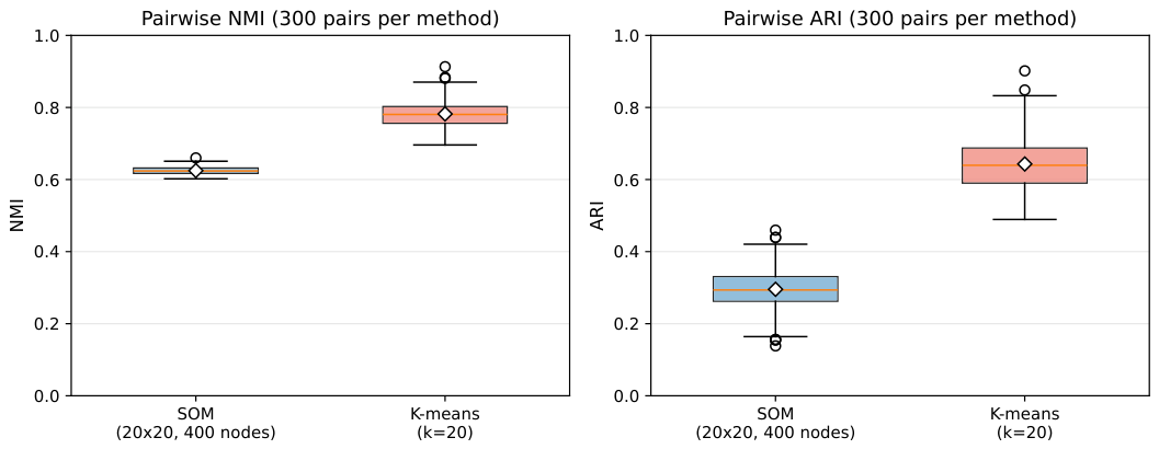
Both methods exhibit non-trivial run-to-run variability, but the magnitude differs substantially. K-means achieves higher pairwise within-method stability than SOMs on both metrics (Table 4, Figure 3).

• K-means: NMI $0.782\pm 0.036$, ARI $0.643\pm 0.071$ (300 pairs).
• SOM: NMI $0.625\pm 0.010$, ARI $0.296\pm 0.057$ (300 pairs).

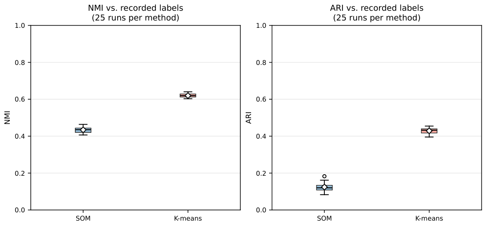
The same ordering holds for agreement with recorded labels (Figure 4).

• K-means: NMI vs. recorded labels $0.620\pm 0.010$, ARI vs. recorded labels $0.429\pm 0.016$.
• SOM: NMI vs. recorded labels $0.434\pm 0.015$, ARI vs. recorded labels $0.124\pm 0.024$.

The distributions are non-overlapping in every case, so the aggregate differences are not attributable to noise; we therefore emphasize their magnitude rather than formal significance testing (full Mann–Whitney and effect-size statistics are provided with the released metrics). The per-cancer and capacity-matched analyses that follow offer a more informative view of the trade-off.

Table 4. Pairwise within-method stability and agreement with recorded labels, mean ± std. Pairwise stability uses $\left({\displaystyle \genfrac{}{}{0pt}{}{25}{2}}\right)=300$ comparisons per method; recorded-label agreement uses 25 replicates per method. K-means values are higher on every aggregate metric. Bold values indicate the higher value between the two methods for each metric.

Method	Pairwise Within-Method		vs. Recorded Labels
	NMI	ARI	NMI	ARI
SOM ($20\times 20$)	$0.625\pm 0.010$	$0.296\pm 0.057$	$0.434\pm 0.015$	$0.124\pm 0.024$
K-means ($k=20$)	$\mathbf{0}.\mathbf{782}\pm \mathbf{0}.\mathbf{036}$	$\mathbf{0}.\mathbf{643}\pm \mathbf{0}.\mathbf{071}$	$\mathbf{0}.\mathbf{620}\pm \mathbf{0}.\mathbf{010}$	$\mathbf{0}.\mathbf{429}\pm \mathbf{0}.\mathbf{016}$

Table 4. Pairwise within-method stability and agreement with recorded labels, mean ± std. Pairwise stability uses $\left({\displaystyle \genfrac{}{}{0pt}{}{25}{2}}\right)=300$ comparisons per method; recorded-label agreement uses 25 replicates per method. K-means values are higher on every aggregate metric. Bold values indicate the higher value between the two methods for each metric.

Method	Pairwise Within-Method		vs. Recorded Labels
	NMI	ARI	NMI	ARI
SOM ($20\times 20$)	$0.625\pm 0.010$	$0.296\pm 0.057$	$0.434\pm 0.015$	$0.124\pm 0.024$
K-means ($k=20$)	$\mathbf{0}.\mathbf{782}\pm \mathbf{0}.\mathbf{036}$	$\mathbf{0}.\mathbf{643}\pm \mathbf{0}.\mathbf{071}$	$\mathbf{0}.\mathbf{620}\pm \mathbf{0}.\mathbf{010}$	$\mathbf{0}.\mathbf{429}\pm \mathbf{0}.\mathbf{016}$

Figure 3. Pairwise within-method stability distributions over 300 pairs per method. K-means has higher and tighter NMI and ARI distributions than SOMs. Blue boxes denote SOMs and orange boxes denote K-means; horizontal lines mark medians, diamonds indicate means, and circles indicate outliers.

Figure 3. Pairwise within-method stability distributions over 300 pairs per method. K-means has higher and tighter NMI and ARI distributions than SOMs. Blue boxes denote SOMs and orange boxes denote K-means; horizontal lines mark medians, diamonds indicate means, and circles indicate outliers.

Figure 4. Per-replicate agreement with recorded cancer type labels across 25 runs per method. K-means achieves higher aggregate NMI and ARI than SOMs. Blue boxes denote SOMs and orange boxes K-means; lines indicate medians, diamonds means, and circles outliers.

Figure 4. Per-replicate agreement with recorded cancer type labels across 25 runs per method. K-means achieves higher aggregate NMI and ARI than SOMs. Blue boxes denote SOMs and orange boxes K-means; lines indicate medians, diamonds means, and circles outliers.

4.2.1. Why K-Means Appears More Stable

A 20-cluster K-means partition admits far fewer distinct assignment configurations than a 400-node SOM partition, so there are correspondingly fewer ways for two runs to disagree. The NMI and ARI both penalize disagreement at the assignment level, and a small initialization shift in the SOM that moves a sample from node $(i,j)$ to neighboring node $(i,j+1)$ is counted as a disagreement even though the topological distance is minimal. K-means’ coarser partition is fundamentally more robust to small perturbations because there are fewer ways to disagree. The objective of SOMs is topology preservation rather than direct partition equivalence with K-means, so raw aggregate metrics that penalize fine-grained disagreement do inflate the apparent gap when the two methods are compared at unequal cardinality. The decisive test, however, is to compare them at matched cardinality: as the capacity-matched curves in Section 4.3 show, the stability gap does not close when the SOM is given the same number of prototypes as K-means—K-means is more reproducible at every matched budget. The granularity argument therefore explains part of the raw gap but not its existence; a real residual difference remains once capacity is controlled. The per-cancer analysis in Section 4.4 reveals what the aggregate metrics conceal about minority classes.

4.2.2. Granularity-Matched Comparison: SOM-Super20

To test whether granularity alone explains the gap, we cluster each SOM’s 400 codebook vectors into 20 superclusters as described in Section 3.6. SOM-Super20 partially closes the ARI gap (pairwise ARI rises from $0.296$ to $0.370$; ARI vs. recorded labels from $0.124$ to $0.264$) but barely changes the NMI (pairwise NMI $0.625\to 0.565$; NMI vs. recorded labels $0.434\to 0.411$).

4.2.3. Why ARI Improves More than NMI Under Coarsening

ARI is defined on pair-level co-assignment counts and is corrected for chance against random partitions of the same cardinality. Reducing a partition from 400 cells to 20 dramatically increases the number of sample pairs that fall into the same cell, which raises both the observed pair agreement and the expected-by-chance pair agreement, but the former rises faster, yielding a higher ARI. NMI, by contrast, is an information-theoretic ratio: $I(U,V)/\sqrt{H\left(U\right)H\left(V\right)}$. Both the mutual information I and the marginal entropies H change when the partition is coarsened, and they tend to change in similar proportions, so the ratio is approximately preserved. The ARI/NMI divergence under SOM-Super20 is therefore expected and reinforces the granularity interpretation: ARI is the metric that visibly tracks partition cardinality, while NMI is the metric that more closely tracks the underlying clustering structure independently of cardinality.

Critically, even at matched granularity, K-means is still decisively superior (pairwise NMI/ARI of $0.782/0.643$ vs. SOM-Super20’s $0.565/0.370$). The conclusion is that K-means’ aggregate stability advantage is not solely a partition granularity artifact; it reflects the fundamental algorithmic difference between density-driven centroid placement and topology-preserving lattice training.

4.3. Capacity-Matched Scaling: Stability at Equal Prototype Budgets

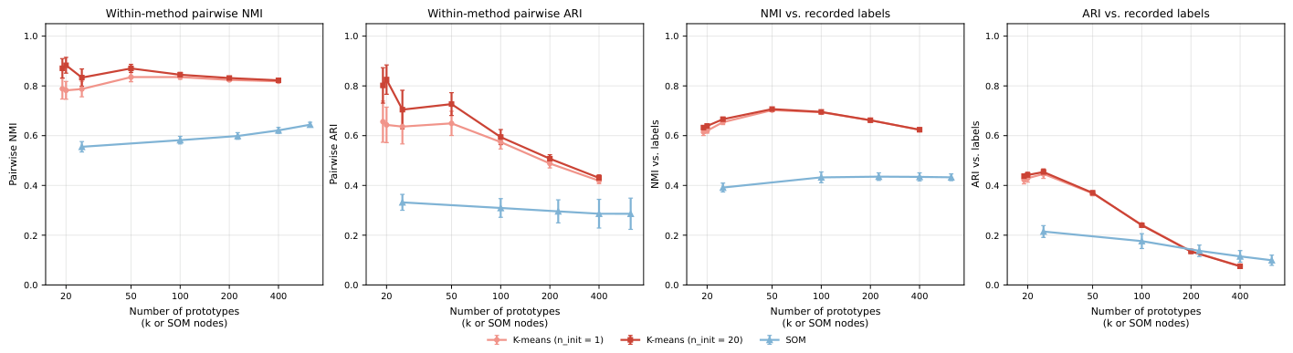
The SOM-Super20 control matches the granularity at a single point (20 prototypes). The capacity sweep generalizes this to the whole range, comparing K-means and SOMs on a shared prototype count axis (Figure 5,

Table 5. Within-method pairwise stability as a function of cluster cardinality (K-means k; SOM lattice nodes), n_init = 1 for K-means, mean over $\left({\displaystyle \genfrac{}{}{0pt}{}{25}{2}}\right)=300$ pairs. K-means is more stable than SOMs at every matched prototype budget; K-means’ pairwise ARI falls as k grows, while NMI is preserved. Table 4 reports the reference MiniSom operating-point runs, whereas the SOM values in this capacity sweep come from independently trained PyTorch/GPU runs, as described in Section 3.3.

Method	Prototypes	Pairwise NMI	Pairwise ARI
K-means $k=19$	19	0.789	0.656
K-means $k=20$	20	0.782	0.643
K-means $k=25$	25	0.787	0.637
K-means $k=50$	50	0.835	0.649
K-means $k=100$	100	0.835	0.574
K-means $k=200$	200	0.824	0.488
K-means $k=400$	400	0.819	0.419
SOM $5\times 5$	25	0.555	0.332
SOM $10\times 10$	100	0.582	0.309
SOM $15\times 15$	225	0.599	0.296
SOM $20\times 20$	400	0.621	0.286
SOM $25\times 25$	625	0.644	0.286

). Two aspects stand out. First, K-means is more reproducible than SOMs at every matched capacity: at $\approx 100$ prototypes, K-means’ pairwise NMI is $0.835$ vs. SOMs’ $0.582$, and, at $\approx 400$, it is $0.819$ vs. $0.621$. SOMs never attain K-means’ stability at any size tested, which confirms—now without the granularity confound—that the stability gap is algorithmic and not an artifact of cardinality.

Second, K-means’ own stability is not uniform in k. The pairwise NMI is essentially flat-to-rising across the range ($0.78\to 0.84\to 0.82$), but the pairwise ARI falls substantially as k grows, from $0.643$ at $k=20$ to $0.419$ at $k=400$. This is the same cardinality effect documented for SOM-Super20 in Section 4.2, running in the opposite direction: raising k multiplies the ways in which a partition can be split, which the pair-counting ARI penalizes while the information-theoretic NMI, which is robust to cardinality, does not. This divergence matters because, as Section 4.4 shows, the high-k regime is exactly where K-means recovers minority classes—so minority recovery is achieved at a measurable cost in ARI stability, representing the core of the three-way trade-off.

4.4. Per-Cancer Trade-Off: Minority Recovery Is Governed by Capacity and Not Topology

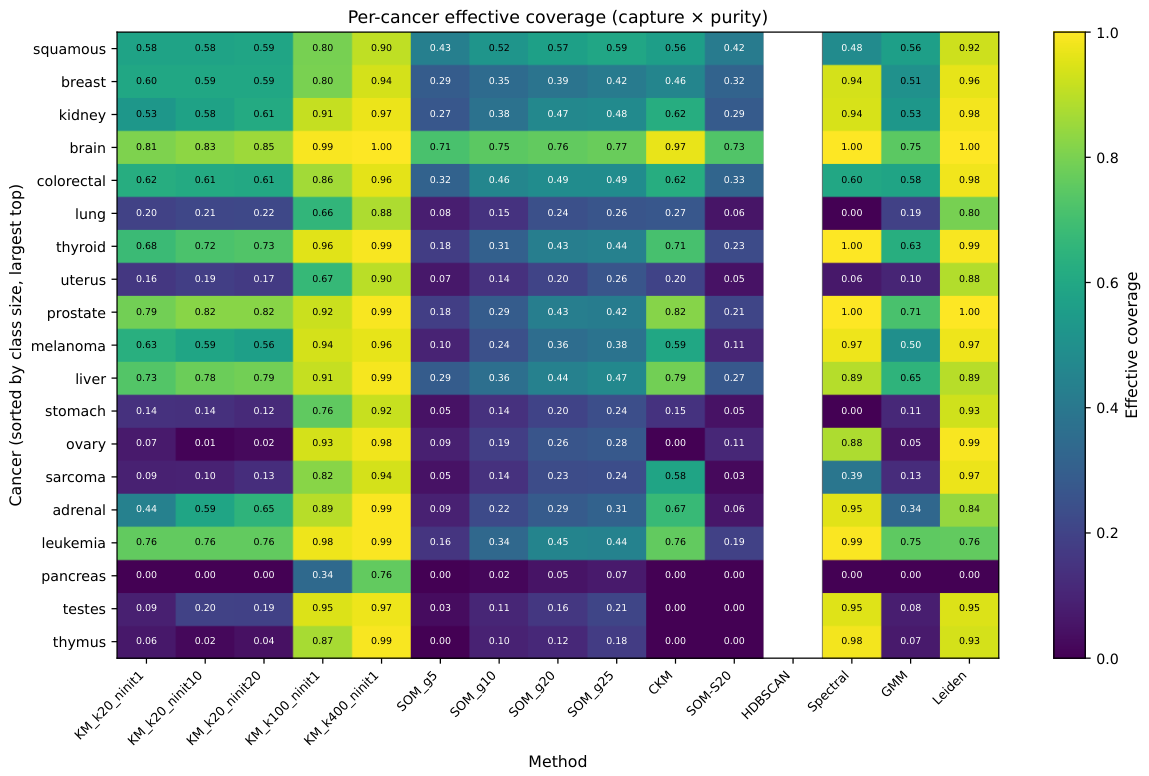
The per-cancer analysis overturns the conclusion that a single-capacity comparison ($k=20$ vs. a $20\times 20$ SOM) would invite. Examined across the full capacity range (Figure 6; minority detail in

Table 6. Effective coverage ($E=\overline{\rho }·\overline{\pi }$, capture × purity) on the three most challenging minority classes, across all evaluated methods and capacities. K-means and SOM values aggregate over 25 seeds (n_init = 1 for K-means unless noted); consensus K-means and SOM-Super20 are post hoc; HDBSCAN is the best of four density settings; deterministic methods are run once. At matched 400 prototypes, K-means exceeds SOMs 6–$14\times$, SOMs do not close the gap even at 625 nodes, and pancreas is recovered only by high-capacity K-means. Bold values indicate the highest effective coverage in each minority-class column.

Method	Prototypes	Pancreas	Testes	Thymus
		($\mathit{n}=\mathbf{151}$)	($\mathit{n}=\mathbf{110}$)	($\mathit{n}=\mathbf{106}$)
SOM $5\times 5$	25	0.000	0.032	0.000
SOM $10\times 10$	100	0.017	0.109	0.096
SOM $20\times 20$	400	0.054	0.163	0.117
SOM $25\times 25$	625	0.072	0.207	0.177
K-means $k=20$ (n_init = 1)	20	0.000	0.088	0.063
K-means $k=20$ (n_init = 20)	20	0.000	0.193	0.043
K-means $k=100$	100	0.342	0.947	0.870
K-means $k=400$	400	0.760	0.973	0.991
Consensus K-means	20	0.000	0.000	0.000
SOM-Super20	20	0.000	0.000	0.000
HDBSCAN (best of 4)	—	0.000	0.000	0.000
Gaussian mixture	20	0.000	0.085	0.073
Spectral	20	0.000	0.952	0.981
Leiden	—	0.000	0.946	0.935

and Figure 7), in this dataset and under the evaluated capacity-matched configurations, minority class recovery tracks the prototype budget and centroid allocation freedom rather than topology preservation. The clearest evidence is for the three most challenging minority classes—pancreas ($n=151$), testes ($n=110$), and thymus ($n=106$)—across matched capacities.

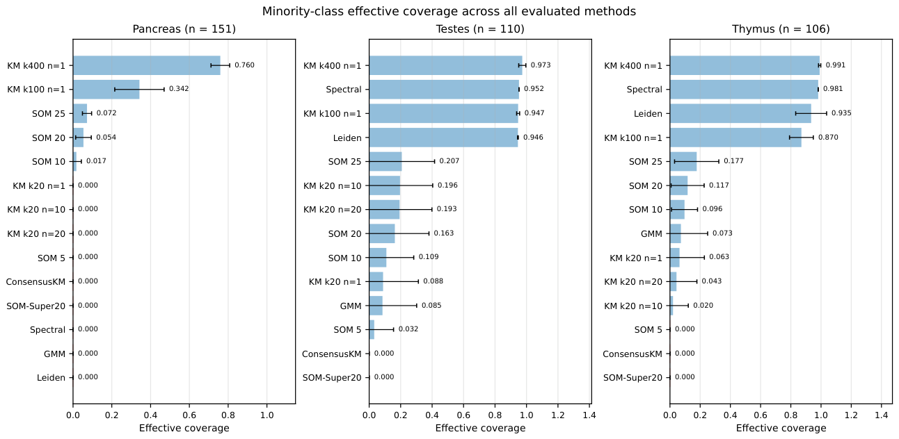
At a matched budget of 400 prototypes, unconstrained K-means recovers these classes 6–$14\times$ more effectively than the lattice-constrained SOM: pancreas effective coverage $0.760$ (K-means $k=400$) vs. $0.054$ (SOM, 400 nodes); testes $0.973$ vs. $0.163$; thymus $0.991$ vs. $0.117$. Recovery rises monotonically with capacity for both methods, but the levels are not comparable: K-means at only 100 prototypes already reaches pancreas $0.342$, testes $0.947$, and thymus $0.870$, while the SOM does not approach these values at any size. Decisively, the SOM at 625 nodes—more prototypes than K-means $k=400$—still recovers pancreas at only $0.072$, whereas K-means with fewer prototypes reaches $0.760$. Capacity alone therefore cannot explain the SOM’s deficit; the binding difference is allocation freedom. K-means may place an unconstrained centroid directly onto a small, dense minority clump, whereas the SOM’s prototypes are tied to a smooth two-dimensional neighborhood and cannot concentrate on a minority without dragging neighboring nodes along, so the class is absorbed into majority-dominated territory. The very constraint that produces SOMs’ interpretable topology is what suppresses their minority recovery.

This reverses the prior interpretation. Earlier single-capacity work—including our own Part 1 framing—suggested that SOMs’ larger node budget conferred a minority advantage. The capacity-matched comparison shows the opposite: whatever budget the SOM is given, an unconstrained centroid method given the same budget recovers minorities far better. The SOM’s per-class contribution is therefore not recovery but the interpretable visualization analyzed in Section 4.5 and Section 4.6.

4.4.1. Consensus K-Means Improves Agreement but Not Recovery

A natural concern is that single-run K-means is an unfair baseline, since consensus clustering is the standard remedy for initialization instability [7]. We therefore evaluated consensus K-means directly (Section 3.5). It achieved the highest aggregate agreement with recorded labels among all evaluated methods (NMI vs. recorded labels $0.649$, ARI vs. recorded labels $0.475$), yet it recovered none of the three most challenging minorities: pancreas, testes, and thymus all indicated zero effective coverage (Table 6).

The mechanism is consistent with the capacity account. Consensus is built at $k=20$ and averages across runs, amplifying assignments that recur and suppressing intermittent ones; it neither adds prototypes nor relaxes allocation, so it has no means of surfacing a small dense minority that the underlying $k=20$ partitions miss. The practical lesson is therefore the opposite of the usual statement: the remedy for missing minorities is not consensus averaging—which sharpens the inequity by removing intermittent minority capture—but raising the capacity, i.e., increasing k (Table 6).

4.4.2. Collapsing SOM to 20 Prototypes Removes Any Recovery

The SOM-Super20 control reduces each 400-node SOM to 20 superclusters via codebook K-means (Section 3.6). Pancreas, testes, and thymus all fall to zero effective coverage under SOM-Super20, matching the single-run case and consensus K-means at the same budget. This is consistent with the capacity account from the opposite direction: lowering the prototype budget removes recovery regardless of whether the prototypes were placed by a lattice or by centroids. Topology preservation still organizes the latent space for visualization, but it confers no minority recovery benefit once the budget is controlled.

4.4.3. The Pattern Holds Across Modern Baselines

To confirm that the conclusion is not specific to the K-means/SOM pair, we compare four widely used methods on the same three minorities (Table 6, Figure 7). The result is sharply method- and class-specific. Spectral clustering and Leiden recover testes ($0.952$ and $0.946$) and thymus ($0.981$ and $0.935$) at levels comparable to high-capacity K-means but recover pancreas at exactly zero. HDBSCAN (all four density settings) and Gaussian mixtures recover none of the three at a usable level. Across every method evaluated—SOMs at any size, consensus K-means, SOM-Super20, HDBSCAN, Gaussian mixtures, spectral clustering, and Leiden—pancreas is recovered only by high-capacity K-means. Pancreas is thus not merely a small class but an allocation stress test: a dense, compact minority that only an unconstrained, high-budget centroid method isolates, while graph- and density-based methods that recover the other two minorities still miss it entirely.

4.4.4. Note on Dominant Cluster Purity

Several K-means entries show very high mean purity (e.g., leukemia $1.000\pm 0.000$, adrenal $0.969\pm 0.077$). When K-means produces a class-dominant cluster, the cluster tends to be highly compact. However, purity alone does not reflect whether the method consistently represents the class. A method capturing 0% of pancreas with undefined purity is not preferable to a method capturing 13% with purity $0.40$. The effective coverage metric combines both capture and purity into a single bounded quantity, allowing a fair comparison across methods and cancer types.

4.4.5. Robustness to k and to the Choice $k=20$

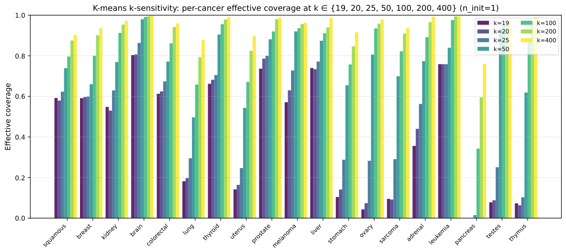
The per-cancer effect of the cluster count is shown in Figure 8. Minority recovery rises monotonically with k for K-means, confirming that the high-k advantage seen in Table 6 is a smooth capacity effect rather than an artifact of a single k. At the low end, $k=19$ (one cluster per cancer type) and $k=20$ (the value inherited from Part 1) are statistically indistinguishable in aggregate stability (pairwise NMI $0.789$ vs. $0.782$; ARI $0.656$ vs. $0.643$) and in minority coverage, so the choice between them does not affect any conclusion; we retain $k=20$ for continuity with Part 1 while reporting the full sweep.

4.4.6. Robustness to n_init

Increasing the number of K-means++ restarts does not alter the minority conclusion. At $k=20$, pancreas’ effective coverage remains $0.000$ at n_init = 1, 10, and 20, and testes and thymus remain within their single-restart ranges (Figure 7).Multiple restarts stabilize the local optimum that K-means reaches but add no representational capacity, so they cannot yield a dominant cluster for a class in which $k=20$ centroids is too few to isolate; the recovery gap closes only with larger k, not with more restarts. The n_init = 10 and n_init = 20 sweeps therefore reproduce the n_init = 1 qualitative conclusions throughout, and we report n_init = 1 as the primary per-seed operating point for the reasons given in Section 3.4.

4.5. Global Topology of the Operating-Point SOM

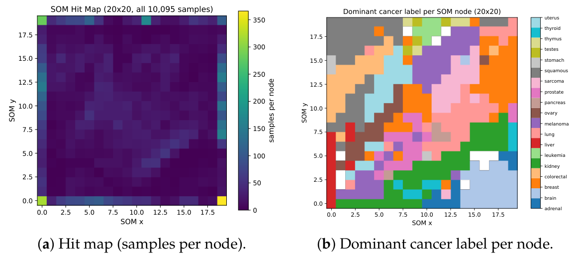
The dominant label map (Figure 9b) demonstrates that the 19 cancer types are organized into spatially coherent territories on the lattice without label supervision: brain in the bottom-right corner; kidney as a diagonal band; liver on the left edge; squamous in the upper left; and lung and melanoma in distinct mid-lattice territories. This emergent spatial coherence is a direct consequence of topology preservation and represents information that K-means’ flat partition cannot represent.

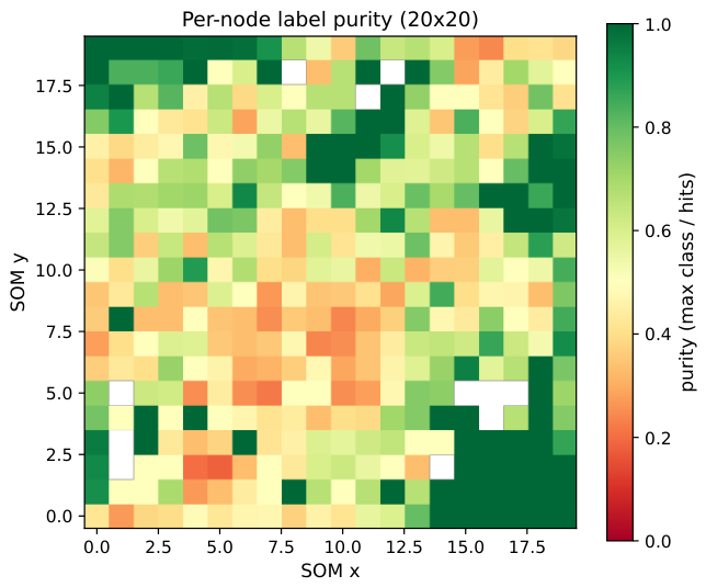
The hit map (Figure 9a) reveals the border attraction artifact characteristic of rectangular SOMs: corner and edge nodes carry disproportionate sample density because they have fewer competing neighbors [16]. We discuss this limitation in Section 5.3. The corresponding per-node label purity map is shown in Figure 10.

4.6. Per-Cancer Case Studies

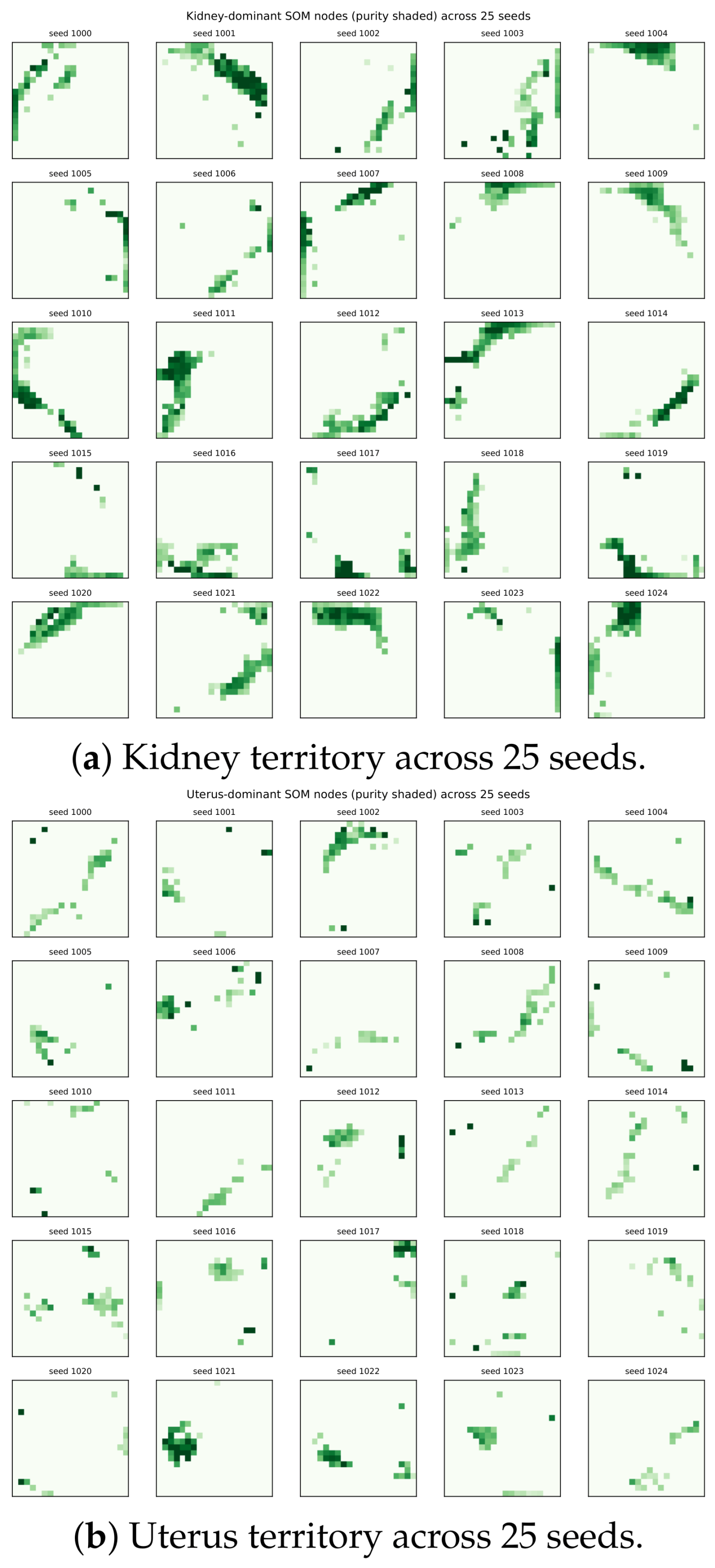
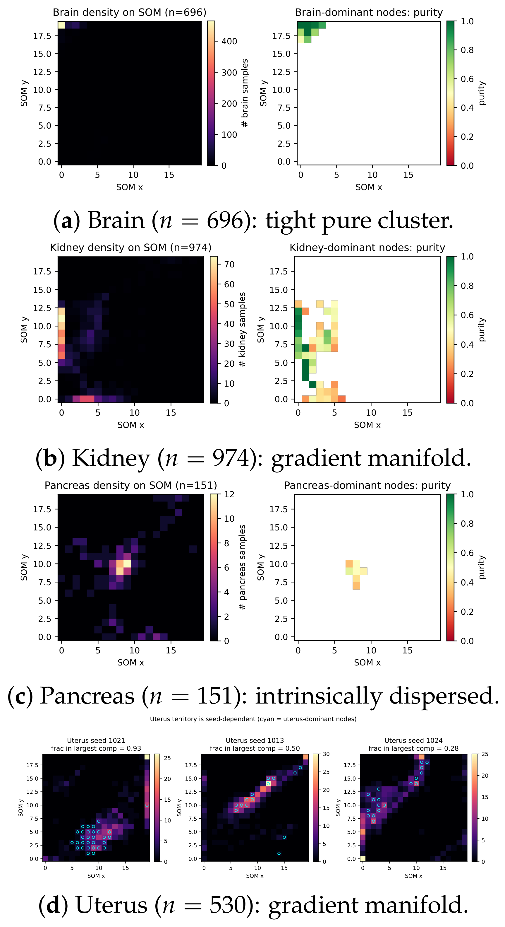
The seed-level reproducibility of the gradient territories is summarized in Figure 11 and quantified here. A representative operating-point ($20\times 20$) SOM illustrates three qualitatively different transcriptomic organizations on the lattice (Figure 12). Brain ($n=696$, Figure 12a) is the tight pure cluster archetype: samples are concentrated in one corner with $91.5\%$ in dominant nodes and mean purity $0.95$, consistent with prior reports of brain tumor expression coherence [32]. Kidney ($n=974$, Figure 12b) and uterus ($n=530$, Figure 12d) form gradient manifolds—continuous diagonal bands rather than discrete regions. This is an SOM-specific view that a flat partition cannot produce; K-means isolates these classes into discrete clusters but cannot represent the continuous transition between neighboring sample compositions. Pancreas ($n=151$, Figure 12c) is the intrinsically dispersed archetype: its samples spread across the lattice without forming a single dominant territory. The correct reading of this panel, in light of Section 4.4, is important: the SOM visualizes that pancreas is dispersed, but it does not recover it. High-capacity K-means isolates pancreas into pure clusters (effective coverage up to $0.760$ at $k=400$), while the SOM map merely makes its dispersion legible. The two roles are complementary: K-means recovers the class; the SOM explains why it is difficult to recover.

Gradient Territories Are Reproducible for Kidney and Seed-Dependent for Uterus

Because our thesis is that a single-seed structure is not by itself trustworthy, we quantify the gradient territories across all 25 operating-point seeds using the coherence analysis of Section 3.11 (Figure 11). Kidney’s dominant nodes form a single coherent component on the majority of seeds: the fraction of dominant nodes in the largest connected component is $0.73\pm 0.20$, and 14 of 25 seeds exceed the $70\%$ coherence threshold, with elongated bounding boxes (aspect ratio $2.36\pm 1.55$) consistent with a diagonal band. Uterus is markedly less reproducible: coherence $0.52\pm 0.17$, with only 3 of 25 seeds above the threshold and near-isotropic bounding boxes ($1.51\pm 0.50$). This indicates that, on most seeds, the uterus territory fragments into several patches rather than one band. The gradient manifold interpretation is therefore well supported for kidney and only weakly, seed-dependently supported for uterus—a distinction that a single-seed figure would have obscured and one that we report explicitly, in line with the multi-seed standard that our work advocates for.

5. Discussion

5.1. The Trade-Off Made Explicit

The experiments characterize a three-way trade-off among partition stability, minority recovery, and topological interpretability that no single method resolves. K-means is the most reproducible method at every matched capacity and, at high capacity, is also the best at recovering minority classes—but its pairwise ARI stability degrades as k grows, so recovery and reproducibility compete against each other within the same method. SOMs are neither the most stable nor the best at recovery at any capacity; their distinctive contribution is the interpretable two-dimensional visualization that neither K-means nor the graph- and density-based baselines provide.

The mechanism behind the minority result is allocation freedom, not the prototype count. K-means may place an unconstrained centroid wherever density warrants, so, given enough centroids, it drops one directly onto a small dense minority. The SOM must keep its prototypes arranged on a smooth lattice, so a node cannot specialize to a minority without pulling its neighbors along; the minority is absorbed into a majority-dominated territory regardless of how many nodes the lattice has. The capacity-matched curves make this concrete: the SOM at 625 nodes still fails to recover pancreas, while K-means at 400 succeeds, and the SOM-Super20 and consensus controls—both fixed at 20 prototypes—fail in the same way as low-k K-means. The earlier reading, in which the SOM’s node budget granted a minority advantage, does not survive matching capacity: the advantage was an artifact of comparing a 400-prototype SOM against 20-prototype K-means.

From an engineering standpoint, the selection rule is therefore not “K-means for stability, SOM for minorities”. It is to raise the capacity (increase k, or use an unconstrained centroid method) when the goal is to surface rare classes, accepting some loss of ARI-level reproducibility; keep capacity low when the goal is a small, reproducible set of partition labels; and add an SOM when the goal is to see and audit the structure—to recognize that a class is dispersed, or that two classes grade continuously into one another— rather than to recover it. The effective coverage metric introduced in Section 3.10 makes the recovery axis of this choice quantitative.

5.2. Topology Preservation as an Engineering Tool

The kidney and uterus case studies (Figure 12b,d) demonstrate a form of structure that is difficult to represent with flat clustering methods. Rather than forming isolated compact groups, these cancers organize as continuous gradients across the SOM lattice, with neighboring regions containing progressively changing sample compositions instead of sharply separated clusters. We stress, consistent with our work’s own multi-seed standard, that this is a reproducible property for kidney (coherent on $14/25$ seeds) but a seed-dependent one for uterus ($3/25$; Figure 11); the engineering value of the SOM view lies in its ability to surface and then test such structure, not to assert it from a single run.

K-means cannot directly represent this type of organization because every sample must belong to exactly one centroid-defined partition. As a result, continuous transitions are forced into discrete cluster boundaries. The SOM preserves local neighborhood relationships and therefore exposes gradual transitions and spatial continuity that are hidden in flat partitions—a visualization capability, distinct from the recovery and stability axes, that is SOMs’ genuine contribution.

This capability is useful beyond transcriptomics. Many engineering problems contain gradual transitions rather than sharply separated states. Examples include fault progression in industrial systems, condition degradation in predictive maintenance, environmental monitoring, and network behavior analysis. In these settings, the ability to visualize and audit neighborhood relationships may be as important as the partition itself.

5.3. The Border Attraction Artifact

The hit map (Figure 9a) shows increased sample density near the corners and edges of the rectangular SOM lattice. This is a known border attraction artifact in rectangular SOMs. Edge and corner nodes have fewer neighboring nodes and therefore experience less competitive pressure during training, causing them to absorb outlier or boundary samples more frequently [16].

Two common mitigations are a hexagonal topology and toroidal lattices. Hexagonal SOMs increase neighborhood symmetry by giving each interior node six neighbors instead of four, while toroidal SOMs remove border nodes entirely by wrapping the lattice edges together. We did not implement these variants because the current study focused on the stability/recovery/interpretability trade-off under a single standardized SOM configuration. Because both variants remain lattice-constrained, our capacity result predicts that they would reduce edge density effects without closing the minority recovery gap (which is governed by allocation freedom, not the lattice geometry); future work could test this prediction directly.

Importantly, the artifact does not invalidate the central findings of the study. The aggregate stability trends, minority class behavior, and SOM-Super20 observations remain consistent across the evaluated runs. The border effect mainly influences spatial density distribution rather than the overall trade-off interpretation.

5.4. Limitations

Several limitations should be acknowledged.

1.

No external cohort validation.All experiments were performed on a single TCGA-derived expression compendium. Independent validation using ICGC, GEO, or other external datasets would strengthen the generalizability of the findings.

2.

No biological validation. The study evaluates clustering behavior and stability rather than biological significance. We do not perform pathway enrichment, differential expression analysis, or survival analysis on the SOM regions, and we intentionally avoid claiming the discovery of new cancer subtypes.

3.

Cross-implementation scope. We used MiniSom as the reference implementation and an equivalent PyTorch/GPU SOM for the capacity sweep. Their agreement was verified at the $20\times 20$ operating point, but the full lattice-size sweep was not duplicated across multiple independent SOM software packages. Repeating the full sweep with additional implementations such as SOMPY or Kohonen-R would further reduce the risk of implementation-specific artifacts.

4.

Dependence on recorded labels. Agreement with recorded cancer type labels is used only as an external reference point rather than a definitive ground truth. The pairwise within-method stability analysis is less sensitive to this limitation because it evaluates reproducibility independently of label trust.

5.

Computational cost. SOM training remains computationally expensive compared to K-means. With the reference CPU implementation, the 25-seed $20\times 20$ SOM protocol required approximately $8.7$ h total wall time, whereas the equivalent K-means experiments required approximately 4 min. The extended 125-map capacity sweep was therefore performed using the equivalent GPU-accelerated PyTorch implementation on an NVIDIA L40S. Larger stability studies would continue to benefit from GPU acceleration or optimized SOM implementations.

5.5. Generality of the Framework for Engineering AI

5.5.1. Scope of the Contribution

We are deliberately specific about what this paper claims, because the object of study is a methodology rather than a domain result. The contribution is an evaluation framework together with a set of algorithmic findings—that minority recovery is governed by the prototype budget and centroid allocation freedom, that consensus averaging sharpens rather than resolves minority inequity, and that partition granularity inflates raw stability comparisons unless capacity is matched. Each of these is a property of the clustering algorithms and the geometry of the data, and each is established here without appeal to biological semantics: the mechanisms invoked—an unconstrained centroid can specialize to a dense minority clump; a lattice-tied prototype cannot without dragging its neighbors; averaging suppresses intermittent structure—are statements about optimization on a generic $N\times D$ imbalanced feature matrix and not gene expression. We therefore position this work as a methodological framework validated on a representative high-dimensional imbalanced test bed, not as a demonstration of engineering deployment. Transfer to specific engineering domains is stated throughout as a hypothesis to be tested (Section 1.3 and Section 6); we add no engineering data and claim no engineering result here.

5.5.2. Why a Transcriptomic Test Bed Is Appropriate for a Methodology Paper

Establishing a methodology of this kind requires data that exhibit the target structural regime: high dimensionality relative to per-class sample counts, class imbalance spanning more than an order of magnitude, labels of known-but-imperfect reliability, no external ground truth, and enough samples to support 25-seed replication. None of the pipeline components are biology-specific: standardization, capacity-matched operating-point sweeping, multi-seed pairwise stability quantification, the capture–purity–effective-coverage decomposition, the SOM-Super20 granularity control, and the visual diagnostic suite (U-matrix, hit map, dominant label map, purity map) all operate on a generic $N\times D$ feature matrix with optional categorical labels. The TCGA compendium ($\mathrm{10,095}\times \mathrm{13,634}$, 19 classes, ∼14× imbalance) realizes exactly this regime and, being public, supports the full reproducibility that a methods contribution demands—whereas many structurally analogous engineering datasets (proprietary fault logs, access-restricted process monitoring streams) do not. Exercising a data shape-driven methodology on a structurally faithful, reproducible public dataset is the standard way to establish it prior to domain-specific validation, and it is the basis on which we regard this paper as being within scope for a methods-oriented engineering AI venue. Extending this validation across engineering benchmarks is the explicit trajectory of the broader research program of which this paper is the methodological foundation.

5.5.3. Hypothesized Engineering Applications

We have not validated the framework on engineering data; the following are predictions that follow from the structural properties established here—capacity-driven recovery, allocation freedom, the inequity-sharpening behavior of consensus, and the visualization value of topology—and that we expect to hold on high-dimensional imbalanced engineering data. Testing them on a published engineering benchmark is the most direct next step (Section 6). We highlight four representative cases spanning AI in engineering design, analysis, manufacturing, control, and operation.

1.

Industrial fault clustering and condition monitoring (manufacturing, operation). Vibration spectra, current signatures, and acoustic emission features from rotating machinery typically yield high-dimensional ($D\sim {10}^3$–${10}^4$) feature vectors with strongly imbalanced fault classes—healthy operation dominates, and rare faults are critical but underrepresented. Our capacity result predicts that surfacing rare faults requires capacity and allocation freedom: a low-k partition or a lattice-constrained SOM will absorb rare faults into the dominant healthy regime, whereas a high-capacity unconstrained centroid method—or a density/graph method of the kind that recovered two of our three most challenging minorities—is far more likely to isolate them. An SOM adds value here not by recovering the faults but by visualizing the fault manifold for engineer auditing. The effective coverage metric quantifies which faults a given method can be expected to recover at deployment.

2.

Process anomaly detection in continuous manufacturing (analysis, control). Multivariate sensor streams from chemical or semiconductor processes generate high-dimensional, imbalanced data where “normal” operating regimes dominate and anomalous regimes are sparse. The consensus clustering finding—that the standard remedy for K-means instability sharpens rather than resolves minority representation—is directly relevant: practitioners cannot rely on consensus methods alone to surface rare anomalies.

3.

Engineering design space exploration (design). When a design space is sampled densely in some regions and sparsely in others (e.g., parameter studies biased toward feasible operating points), the trade-off between reproducibility and per-region recovery that we quantify here applies to deciding how to characterize the space and at what capacity. An SOM additionally visualizes gradient-organized regions (analogous to our reproducible kidney case) that flat partitions cannot display—which is valuable when adjacent design points must be understood as continuously related rather than categorically distinct, provided that such gradients are confirmed across seeds rather than read from a single run.

4.

Network and system-log analysis (operation, security). Intrusion detection datasets and system-log embeddings exhibit class imbalance (rare attack types) and require interpretable visual auditing of the discovered partition. The SOM-based visualization suite presented here—hit maps and dominant label maps—supports the same auditing role for these data sources.

5.5.4. What Is Domain-Independent and What Is Not

The specific conclusions established here—that minority recovery is governed by capacity and centroid allocation freedom rather than topology, that recovery and ARI-level reproducibility are traded off within a single method as the capacity grows, and that consensus clustering sharpens rather than resolves minority inequity—follow from the structural properties of the algorithms and the shape of the data, not from biological semantics. We therefore expect them to be replicated on engineering datasets with the same structural properties, but we treat this as an expectation to be tested rather than a demonstrated result; validating it on a published engineering benchmark is the most direct extension of this work (Section 6).

6. Future Work

The most direct extensions are (i) validation on a published high-dimensional imbalanced engineering benchmark (e.g., bearing fault vibration or semiconductor process data), to test whether the capacity/allocation and consensus inequity findings transfer beyond transcriptomics; (ii) external cohort validation on ICGC and GEO datasets; (iii) hexagonal or toroidal SOM topologies to mitigate border attraction; and (iv) biological validation through differential expression, pathway enrichment, and clinical outcome analysis. The graph- and density-based methods originally envisioned as corroboration—Leiden and HDBSCAN—are now incorporated directly as baselines (Section 3.7). As a biomedical/transcriptomic extension, we plan to derive compact gene panels (20/50/100-gene signatures) via $L_1$-regularized models for portable subtype scoring on external cohorts.

7. Conclusions

We have presented a capacity-matched characterization of how three properties—partition stability, minority class recovery, and topological interpretability—are traded off across clustering methods for the unsupervised analysis of imbalanced, high-dimensional data, demonstrated on a TCGA-derived RNA expression compendium of $\mathrm{10,095}$ samples spanning 19 cancer types. Comparing K-means ($k\in \{19,\dots ,400\}$) and SOMs (25–625 nodes) at matched prototype budgets, together with consensus K-means, SOM-Super20, and four modern baselines, we find that K-means is more reproducible than SOMs at every matched capacity and that, at high capacity, it also recovers the smallest cancers far better—6–$14\times$ better than SOMs at 400 prototypes, with SOMs failing to close the gap even at 625 nodes. Therefore, minority recovery is, under matched capacity, better explained by representational capacity and centroid allocation freedom than by topology preservation; the earlier impression of an SOM minority advantage was an artifact of comparing methods at unequal capacity. This recovery is not free: raising k overfragments the partition and lowers the pairwise ARI stability ($0.643\to 0.419$ from $k=20$ to $k=400$) while NMI is preserved, so reproducibility and recovery are traded off within K-means itself. Pancreas, the most challenging class, was recovered by no method that we evaluated except high-capacity K-means—not by SOMs at any size, nor by consensus K-means, SOM-Super20, HDBSCAN, Gaussian mixtures, spectral clustering, or Leiden. The SOM’s distinct contribution is neither stability nor recovery but interpretable two-dimensional visualization, including a gradient-organized structure that we show is reproducible across seeds for kidney and seed-dependent for uterus. The choice among methods thus depends on which of the three properties a task prioritizes: reproducibility, minority recovery, or visual interpretability. The per-cancer effective coverage metric that we introduce (capture rate × dominant cluster purity) makes the recovery axis quantitative. We release the full pipeline, all trained model artifacts, and per-run metrics; because the findings follow from the shape of the data and the allocation behavior of the algorithms rather than from biological semantics, we expect—and propose to test—that they transfer to other imbalanced high-dimensional unsupervised problems. We are explicit that this transfer to engineering domains is an expectation grounded in structural properties, not a result demonstrated here: validation on published engineering benchmarks is a necessary next step, and the present paper establishes the methodology and the algorithmic findings on a representative, reproducible test bed that exhibits the target structural regime.

References

1. Ahmed, I.; Soliman, H. Machine learning modeling for identifying cancer subtypes from gene expressions. 2026; Manuscript under review.
2. Wang, Z.; Gerstein, M.; Snyder, M. RNA-Seq: A revolutionary tool for transcriptomics. Nat. Rev. Genet. 2009, 10, 57–63. [Google Scholar] [CrossRef] [Scilit]
3. Tomczak, K.; Czerwińska, P.; Wiznerowicz, M. The Cancer Genome Atlas (TCGA): An immeasurable source of knowledge. Contemp. Oncol./Współczesna Onkol. 2015, 19, A68–A77. [Google Scholar] [CrossRef] [Scilit] [PubMed]
4. Ahn, T.; Goo, T.; Lee, C.H.; Kim, S.; Han, K.; Park, S.; Park, T. Deep learning-based identification of cancer or normal tissue using gene expression data. In Proceedings of the 2018 IEEE International Conference on Bioinformatics and Biomedicine (BIBM); IEEE: Piscataway, NJ, USA, 2018; pp. 1748–1752. [Google Scholar]
5. Lyu, B.; Haque, A. Deep learning based tumor type classification using gene expression data. In Proceedings of the ACM International Conference on Bioinformatics, Computational Biology, and Health Informatics (BCB); ACM: New York, NY, USA, 2018; pp. 89–96. [Google Scholar] [CrossRef] [Scilit]
6. Kodinariya, T.M.; Makwana, P.R. Review on determining number of Cluster in K-Means Clustering. Int. J. 2013, 1, 90–95. [Google Scholar]
7. Monti, S.; Tamayo, P.; Mesirov, J.; Golub, T. Consensus clustering: A resampling-based method for class discovery and visualization of gene expression microarray data. Mach. Learn. 2003, 52, 91–118. [Google Scholar] [CrossRef] [Scilit]
8. Liu, Z.; Zhang, X.; Zhang, S. Breast tumor subgroups reveal diverse clinical prognostic power. Sci. Rep. 2014, 4, 4002. [Google Scholar] [CrossRef] [Scilit] [PubMed]
9. Guo, Y.; Zheng, J.; Shang, X.; Li, Z. A similarity regression fusion model for integrating multi-omics data to identify cancer subtypes. Genes 2018, 9, 314. [Google Scholar] [CrossRef] [Scilit] [PubMed]
10. Kohonen, T. The self-organizing map. Proc. IEEE 1990, 78, 1464–1480. [Google Scholar] [CrossRef] [Scilit] [PubMed][Green Version]
11. Ultsch, A. U*-Matrix: A Tool to Visualize Clusters in High-Dimensional Data; Technical Report 36; Department of Computer Science, University of Marburg: Marburg, Germany, 2003. [Google Scholar]
12. Wirth, H.; Löffler, M.; von Bergen, M.; Binder, H. Expression cartography of human tissues using self organizing maps. BMC Bioinform. 2011, 12, 306. [Google Scholar] [CrossRef] [Scilit] [PubMed]
13. Tamayo, P.; Slonim, D.; Mesirov, J.; Zhu, Q.; Kitareewan, S.; Dmitrovsky, E.; Lander, E.S.; Golub, T.R. Interpreting patterns of gene expression with self-organizing maps: Methods and application to hematopoietic differentiation. Proc. Natl. Acad. Sci. USA 1999, 96, 2907–2912. [Google Scholar] [CrossRef] [Scilit] [PubMed]
14. Gibson, P.B.; Perkins-Kirkpatrick, S.E.; Uotila, P.; Pepler, A.S.; Alexander, L.V. On the use of self-organizing maps for studying climate extremes. J. Geophys. Res. Atmos. 2017, 122, 3891–3903. [Google Scholar] [CrossRef] [Scilit]
15. Kebalepile, M.M.; Dzikiti, L.; Voyi, K. Supervised Kohonen self-organizing maps of acute asthma from air pollution exposure. Int. J. Environ. Res. Public Health 2021, 18, 11071. [Google Scholar] [CrossRef] [Scilit] [PubMed]
16. Ultsch, A.; Lötsch, J. Machine-learned cluster identification in high-dimensional data. J. Biomed. Inform. 2017, 66, 95–104. [Google Scholar] [CrossRef] [Scilit] [PubMed]
17. Lange, T.; Roth, V.; Braun, M.L.; Buhmann, J.M. Stability-based validation of clustering solutions. Neural Comput. 2004, 16, 1299–1323. [Google Scholar] [CrossRef] [Scilit] [PubMed]
18. Ben-Hur, A.; Elisseeff, A.; Guyon, I. A stability based method for discovering structure in clustered data. In Proceedings of the Pacific Symposium on Biocomputing; World Scientific: Singapore, 2002; Volume 7, pp. 6–17. [Google Scholar]
19. Strehl, A.; Ghosh, J. Cluster ensembles—A knowledge reuse framework for combining multiple partitions. J. Mach. Learn. Res. 2002, 3, 583–617. [Google Scholar]
20. Hubert, L.; Arabie, P. Comparing partitions. J. Classif. 1985, 2, 193–218. [Google Scholar] [CrossRef] [Scilit]
21. Castaldi, P.J.; Benet, M.; Petersen, H.; Rafaels, N.; Finigan, J.H.; Paoletti, M.; Boezen, H.M.; Vonk, J.M.; Bowler, R.; Pistolesi, M.; et al. Do COPD subtypes really exist? COPD heterogeneity and clustering in 10 independent cohorts. Thorax 2017, 72, 998–1006. [Google Scholar] [CrossRef] [Scilit] [PubMed]
22. Vesanto, J.; Alhoniemi, E. Clustering of the self-organizing map. IEEE Trans. Neural Netw. 2000, 11, 586–600. [Google Scholar] [CrossRef] [Scilit] [PubMed]
23. Tjoa, E.; Guan, C. A survey on explainable artificial intelligence (XAI): Toward medical XAI. IEEE Trans. Neural Netw. Learn. Syst. 2021, 32, 4793–4813. [Google Scholar] [CrossRef] [Scilit] [PubMed]
24. Holzinger, A.; Langs, G.; Denk, H.; Zatloukal, K.; Müller, H. Causability and explainability of artificial intelligence in medicine. Wiley Interdiscip. Rev. Data Min. Knowl. Discov. 2019, 9, e1312. [Google Scholar] [CrossRef] [Scilit] [PubMed]
25. Vettigli, G. MiniSom: Minimalistic and NumPy-Based Implementation of the Self-Organizing Map. 2018. Available online: https://github.com/JustGlowing/minisom (accessed on 8 May 2026).
26. Campello, R.J.G.B.; Moulavi, D.; Sander, J. Density-Based Clustering Based on Hierarchical Density Estimates. In Proceedings of the Advances in Knowledge Discovery and Data Mining (PAKDD 2013); Lecture Notes in Computer Science; Springer: Berlin/Heidelberg, Germany, 2013; Volume 7819, pp. 160–172. [Google Scholar] [CrossRef] [Scilit]
27. McInnes, L.; Healy, J.; Astels, S. hdbscan: Hierarchical density based clustering. J. Open Source Softw. 2017, 2, 205. [Google Scholar] [CrossRef] [Scilit]
28. von Luxburg, U. A tutorial on spectral clustering. Stat. Comput. 2007, 17, 395–416. [Google Scholar] [CrossRef] [Scilit]
29. Fraley, C.; Raftery, A.E. Model-Based Clustering, Discriminant Analysis, and Density Estimation. J. Am. Stat. Assoc. 2002, 97, 611–631. [Google Scholar] [CrossRef] [Scilit]
30. Traag, V.A.; Waltman, L.; van Eck, N.J. From Louvain to Leiden: Guaranteeing well-connected communities. Sci. Rep. 2019, 9, 5233. [Google Scholar] [CrossRef] [Scilit] [PubMed]
31. Pedregosa, F.; Varoquaux, G.; Gramfort, A.; Michel, V.; Thirion, B.; Grisel, O.; Blondel, M.; Prettenhofer, P.; Weiss, R.; Dubourg, V.; et al. Scikit-learn: Machine Learning in Python. J. Mach. Learn. Res. 2011, 12, 2825–2830. [Google Scholar]
32. Verhaak, R.G.W.; Hoadley, K.A.; Purdom, E.; Wang, V.; Qi, Y.; Wilkerson, M.D.; Miller, C.R.; Ding, L.; Golub, T.; Mesirov, J.P.; et al. Integrated genomic analysis identifies clinically relevant subtypes of glioblastoma characterized by abnormalities in PDGFRA, IDH1, EGFR, and NF1. Cancer Cell 2010, 17, 98–110. [Google Scholar] [CrossRef] [Scilit] [PubMed]
Figure 1. Experimental pipeline. The TCGA expression compendium is preprocessed and used to train the two primary clustering methods (SOM and K-means) across a range of cluster cardinalities under a 25-seed protocol. Two post hoc baselines are derived from the trained models (consensus K-means from the K-means co-assignment matrix and SOM-Super20 from each SOM’s codebook), and four modern clustering baselines (HDBSCAN, spectral, Gaussian mixtures, Leiden) are added for breadth. All methods are evaluated through paired stability metrics, per-cancer effective coverage, and—for the SOM—visual diagnostics. Pipeline scripts and trained artifacts are released for reproducibility.
Aieng 01 00010 g001
Figure 2. U-matrix visualizations across the grid size sweep. Darker cells indicate larger average distances to lattice neighbors (potential boundaries between groups); lighter cells indicate locally homogeneous regions. The 20 × 20 configuration was selected as the operating point.
Aieng 01 00010 g002
Figure 5. Capacity-matched stability scaling for K-means (n_init = 1 and n_init = 20) and SOMs across a shared log-scaled prototype axis, where # denotes SOM nodes. Left panels show within-method pairwise NMI/ARI; right panels show agreement with recorded labels. K-means is more reproducible at every matched budget; its pairwise ARI decreases with increasing k due to overfragmentation, while NMI remains stable.
Aieng 01 00010 g005
Figure 6. Per-cancer effective coverage (capture × purity) for all 19 cancer types (rows, largest at top) across the evaluated methods and capacities (columns). High-capacity K-means (KM_k100/k400) is the only method family with non-zero pancreas coverage and provides strong coverage across all three smallest classes. SOMs provide low but non-zero coverage for testes and thymus; spectral clustering and Leiden also strongly recover testes and thymus but not pancreas.
Aieng 01 00010 g006
Figure 7. Minority class effective coverage across all evaluated methods for the three most challenging classes (pancreas, testes, thymus), sorted within each panel. Bars at zero (highlighted) mark methods that fail to recover the class. Pancreas is recovered only by high-capacity K-means; spectral clustering and Leiden recover testes and thymus but not pancreas.
Aieng 01 00010 g007
Figure 8. K-means per-cancer effective coverage as a function of k ∈ { 19 , 20 , 25 , 50 , 100 , 200 , 400 } (n_init = 1), sorted by class size (largest left). Minority class coverage rises monotonically with k, while majority class coverage is already saturated at small k.
Aieng 01 00010 g008
Figure 9. Global views of the operating-point ( 20 × 20 ) SOM. Panel (a) shows the hit map representing the number of samples mapped to each SOM node. Brighter edge and corner regions illustrate the border attraction behavior commonly observed in rectangular SOM lattices. Panel (b) shows the dominant cancer label associated with each node, demonstrating spatially coherent territories for multiple cancer types across the SOM topology.
Aieng 01 00010 g009
Figure 10. Per-node label purity (maximum class count divided by total node hits). Dark green nodes ( ≥ 0.9 ) are locally homogeneous; orange nodes (0.3–0.5) reflect overlap among multiple cancer types.
Aieng 01 00010 g010
Figure 11. Gradient-territory reproducibility across 25 operating-point ( 20 × 20 ) SOM seeds. Kidney is largely coherent (largest-component fraction 0.73 ± 0.20 ; 14 / 25 seeds ≥ 70 % ), whereas uterus is more fragmented ( 0.52 ± 0.17 ; 3 / 25 ), indicating greater seed dependence. Each panel shows one seed; only cancer-dominant nodes are colored, with darker green indicating higher dominant-label purity.
Aieng 01 00010 g011
Figure 12. Per-cancer case studies on a representative operating-point ( 20 × 20 ) SOM. Each panel contains density visualization and a dominant node purity analysis for the corresponding cancer type. Brain forms a compact and highly pure cluster structure, while kidney and uterus exhibit continuous gradient-like manifold organization across the SOM lattice. Pancreas appears intrinsically dispersed, with samples distributed across multiple regions and without a single dominant territory. Panels show one representative operating-point seed; the seed stability of the kidney and uterus territories across all 25 seeds is quantified in Figure 11. Here, # denotes the number of samples mapped to a node; density-map color scales encode sample counts, purity-map color scales encode dominant-node purity, and in panel (d) cyan circles mark uterus-dominant nodes.
Aieng 01 00010 g012