
Article

Inequality in Survivorship in Midlife in the US
by
Warren Sanderson
1,* and
Sergei Scherbov
2,3
1
Department of Economics, Stony Brook University, Stony Brook, NY 11794-4384, USA
2
Population and Just Societies Program, International Institute for Applied Systems Analysis, A-2361 Laxenburg, Austria
3
College of Population Studies, Chulalongkorn University, Bangkok 10330, Thailand
*
Author to whom correspondence should be addressed.
Trends Public Health 2026, 1(1), 3; https://doi.org/10.3390/tph1010003
Submission received: 10 February 2026 / Revised: 17 March 2026 / Accepted: 26 March 2026 / Published: 31 March 2026

Abstract

Background/Objectives: Inequality in survival across socioeconomic strata has been growing in the US for decades. Traditional measures of this inequality increasingly fail to capture the heterogeneous biological realities of the US population. Using new measures, this study provides a fresh perspective on the dynamics of mortality inequality across ten socioeconomic deciles in the United States from 1982 to 2019. Methods: The data come from annual life tables from US counties, aggregated according to their socioeconomic characteristics. Measures of Inequality: Three measures of inequality are used, capturing survival inequality from different perspectives, inequality in ages of death over the lifecycle, inequality in survival at older ages, and inequality in survival in midlife. For the latter, the equal survivorship age (ESA)—a metric defined as the age at which a specific subgroup’s survival probability from age 20 matches the survival probability from age 20 to 65 of the total population—is used. Results: We find consistently growing inequality, largely unaffected by economic circumstances such as the Great Recession. By 2019, the ESA for the lowest socioeconomic decile was nearly 11 years lower than the ESA of the highest decile. Conclusions: This “survival gap” in the ESA suggests that low-socioeconomic status (SES) populations effectively exhaust their survival reserves a decade earlier than their high SES counterparts. These findings challenge the equity of the use of universal chronological ages in public policies and underscore the need for “Social-Determinant-Adjusted” geriatric policy models. The growing inequality in the ESA suggests the importance of cohort-based influences.

1. Introduction

For nearly a century, the chronological age of 65 has served as the de facto threshold for “old age” in the United States, governing eligibility for Social Security, Medicare, and the focus of geriatric medicine. This uniform boundary assumes a relatively homogeneous aging process across the population. However, recent demographic data indicate that the United States is undergoing a “Great Divergence” in health outcomes, where gains in longevity are disproportionately accrued by the socioeconomically advantaged [1,2,3,4]. This paper applies the Characteristics Approach (CA) framework [5] to U.S. mortality data to challenge the utility of fixed chronological ages in studying heterogeneity in mortality.
The study of mortality inequality over time in the US at the county level was based on earlier work in the UK [6,7]. Carstairs and Morris [7] studied mortality by geographic units in England, Scotland, and Wales around 1981, using a four-dimensional “deprivation score”. Based on that score, geographic units were divided into seven categories from lowest to highest deprivation score. Earnes et al. [6] built on the work of Carstairs and Morris, using three indices of deprivation and different geographic units. Earnes et al. found that their deprivation indices were closely related to all-source mortality as well as mortality from heart disease and from smoking.
In a series of articles, Singh and Siahpush [8,9] applied the UK methodology to US counties using an 11-factor deprivation index. They divided counties into deciles based on their index. Singh and Siahpush found that, for women in the lowest decile, life expectancy at birth was 1.3 years lower than for those in the highest decile in 1980–1982, and fell to 3.3 years lower in 1998–2000. For men, the differences were 3.8 years and 5.4 years, respectively.
Dwyer-Lindgren et al. [10] studied county-level differences in life expectancy at birth from 1980 to 2014. Using principal components methodology, they produced three composite indices, representing socioeconomic race/ethnicity factors, behavioral and metabolic risk factors, and health care factors. The index for socioeconomic race/ethnicity factors included variables for race, ethnicity, education, and income. The index for behavioral and metabolic risk factors included variables for physical activity, obesity, smoking, hypertension, and diabetes prevalence. The index for health care factors included the percentage of the population under 65 insured, a health care quality index, and the number of physicians per 1000 population. In a model of life expectancy at birth, the index for behavioral and metabolic risks and the index for health care were statistically significant, and the index for socioeconomic race/ethnicity factors was not. Adding both the socioeconomic race/ethnic index and health care index to a model with just an intercept and the behavioral and metabolic risk factors did not raise the adjusted R-squared. The conclusion is that the most important factors influencing life expectancy differences across counties were those associated with behavioral and metabolic risks.
Case and Deaton [3,4,11] studied the increasing inequality in health and survival in the US, focusing on the experiences of white non-Hispanics with only a high school education. In [11], they called the increasing deaths in midlife in that group “deaths of despair.” In [3], they looked at possible causes of the increasing divergence of the mortality rates of white non-Hispanics and other Americans, ranging from increasing income inequality to decreasing access to healthcare. They found that they were not a satisfactory explanation. They produced a tentative possible explanation that they labeled “cumulative disadvantage.” “Cumulative disadvantage” was said to be due to the continuing worsening of the labor market conditions of white non-Hispanics at the time of labor market entry. These worsening conditions had cumulative effects from less investment in human capital to less stable family structures.
Case and Deaton’s view of “cumulative disadvantage” is related to the “weathering” hypothesis [12,13], which posits that the cumulative stress of socioeconomic disadvantage accelerates cellular aging. This results in an earlier onset of chronic disease and frailty for low-SES individuals. Consequently, chronological age becomes a poor proxy for biological age, as the “biological clocks” of the rich and poor run at different speeds [14].
The object of this paper is to analyze survival inequality from three perspectives: (1) inequality in survival over the lifecycle, (2) inequality in survival at older ages and (3) inequality in survival in midlife. Inequality in survival over the lifecycle is quantified using the Human Life Indicator (HLI) [15]. Inequality in survival for older adults is quantified using the Prospective Old Age Threshold (POAT) [5]. Both the HLI and the POAT have previously been used to analyze inequality. Here we introduce and emphasize a new measure to complement them, the Equal Survivorship Age (ESA). The ESA measures survival inequality in midlife. In combination with the HLI and the POAT, it provides an important new perspective on the dynamics of survival inequality. The ESA translates differences in survivorship in midlife into a readily interpretable age metric, which complements rather than duplicates the information provided by the other two measures.
Data on life expectancy at birth reveal one dimension of inequality but hide another one. Life expectancy is the arithmetic average age at death in a life table population. Two arithmetic averages can be the same, but the variability in ages of death over the life cycle could be different. To address differences in the variability of ages of death, Ghislandi, Sanderson, and Scherbov [15] developed the Human Life Indicator (HLI). The HLI is the geometric mean of ages at death in a life table population. It reflects both the arithmetic average age at death and the variation in those ages. The difference between life expectancy at birth and the HLI is a measure of that variation. Larger variations in ages at death result in larger differences between life expectancy at birth and the HLI. An observation with a larger difference would reflect a case where deaths are more concentrated at the earliest and latest portions of the life cycle. An observation of a smaller difference would reflect a case where ages at death were more concentrated.
Van Raalte et al. [16] argue for the importance of studying the variability in ages at death (lifespan inequality) in addition to life expectancy. Sasson [17] showed how life expectancy and lifespan inequality (measured by the standard deviations in ages at death) changed in the US from 1990 to 2010 by educational attainment.
The traditional approach to the study of population aging is increasingly criticized for focusing on chronological age rather than functional ability [18]. Sanderson and Scherbov [5,19,20,21] introduced the concept of Prospective Old Age Threshold. It is the age at which the average remaining life expectancy first falls below 15 years. In contrast to a threshold based on a fixed chronological age, such as 65, this threshold of old-age varies across socio-economic conditions and over time. As populations become healthier, the POAT rises, signaling that the onset of “old age” is being delayed. The inequality in POATs expresses the inequality of the onset of “old age”.

2. Materials and Methods

2.1. Data

We utilized a longitudinal dataset of U.S. county life tables from 1982 to 2019, produced for the Society of Actuaries [22,23]. The methodology that was used to produce it was an extension of that in Singh [8,9]. A socioeconomic index score (SIS) is computed for each county in each year. The values of the SIS in 2000 are used to aggregate counties into deciles of equal population size in that year, and the distribution of counties into deciles is then fixed for the entire period (1 = lowest, 10 = highest, “All” = the total population).
The SIS is based on the normalized values of 11 variables:
  • Percentage of the population aged 25 and over with less than 9 years of education.
  • Percentage of the population aged 25 and over with at least 4 years of college education.
  • Percentage of the population aged 16 and over employed in a white-collar occupation.
  • Unemployment rate for the population 16 years and over.
  • Median household income adjusted for local housing costs.
  • Ratio of the average household income in the lowest quintile to the average household income in the highest quintile.
  • Percentage of the population below the federal poverty threshold.
  • Median home value for owner-occupied units.
  • Median gross rent for rental units.
  • Percentage of housing without a telephone.
  • Percentage of housing without complete plumbing.
The normalized values are combined based on weights derived from a principal components analysis.
County-level mortality data are derived from the National Center for Health Statistics, and county-level population distributions are derived from the US Decennial Census and the American Community Survey. We had no choice in the methodology used to create the life tables produced by the Society of Actuaries, and have no way to alter any of the features of that methodology. Two aspects of that methodology are especially important here. First, the assignment of counties to deciles remains constant over time. This allows our measures to be temporally consistent. Second, the methodology of producing life tables using these data is the same as that used to produce the life tables in the Human Mortality Database. This permits the US data to be analyzed in an international perspective. The methodology used to produce the life tables here and in the Human Mortality Database is generally considered to be of the highest quality. The full description of the methodology used to produce the life tables can be found in [23].

2.2. Key Measures

We employ three measures of population aging that account for heterogeneity: the Human Life Indicator (HLI), the Prospective Old Age Threshold (POAT), and the Equal Survivalship Age (ESA). The HLI measures survival over the lifecycle. The POAT measures survival rates at older ages, and the ESA shows the heterogeneity of survival rates in midlife.

2.2.1. Human Life Indicator (HLI)

Life expectancy at birth is the arithmetic average of ages at death in a life table population. The HLI is the geometric average of ages at death in a life table population. We use it to detect heterogeneity that is manifested as increases in lifespan inequality. When the age pattern of deaths shifts so that the variance in the age at death increases, the HLI falls relative to life expectancy at birth.

2.2.2. Prospective Old-Age Threshold (POAT)

The age x where remaining life expectancy is 15 years: In standard life table notation:
e(x) = 15 years.
We use the POAT to assess trends in the heterogeneity of aging at older ages.

2.2.3. Equal Survivorship Age (ESA)

We introduce this measure here to assess changes in the pattern of survival rate changes for people in midlife. It is the age in the population under study at which the probability of surviving from age 20 to that age is the same as the probability of surviving from age 20 to age 65 in the aggregate population of the same year (the total population in all the deciles). Because it is benchmarked against a moving national standard, the ESA provides a detrended measure of inequality across the deciles.
In standard life table notation, the ESA for decile d in year t is x where
l x , t , d l 20 , t , d = l 65 , t , U S l 20 , t , U S ,
where l x , t , d is the proportion of the life table population of decile d in year t that survives to age x, and l x , t , U S is the proportion of the life table population of the US in year t that survives to age x. When age x is not an integer value, spline interpolation is used to compute it. Age 65 was chosen because it remains the historically and institutionally salient threshold of “old age” in the United States, especially in relation to retirement, healthcare, and other public policies.

3. Results

3.1. Inequality over the Lifecycle

The “Great Divergence” is clearly visible in Figure 1 below. For clarity, in all our Figures, we show only the lowest and the highest decile for both sexes combined. In 1982, the gap in life expectancy at birth between Decile 1 (72.9 years) and Decile 10 (75.8 years) was roughly 3 years. By 2019, this gap widened to 6.6 years, with life expectancy in decile 10 reaching 82.4 years while Decile 1 increased more slowly to 75.8 years. Between 2010 and 2019, life expectancy at birth for the entire population stagnated. The stagnation in life expectancy growth observed in the aggregate was a result of life expectancy at birth falling for the least advantaged groups, increasing for the most advantaged, and remaining little changed for the groups in the middle.
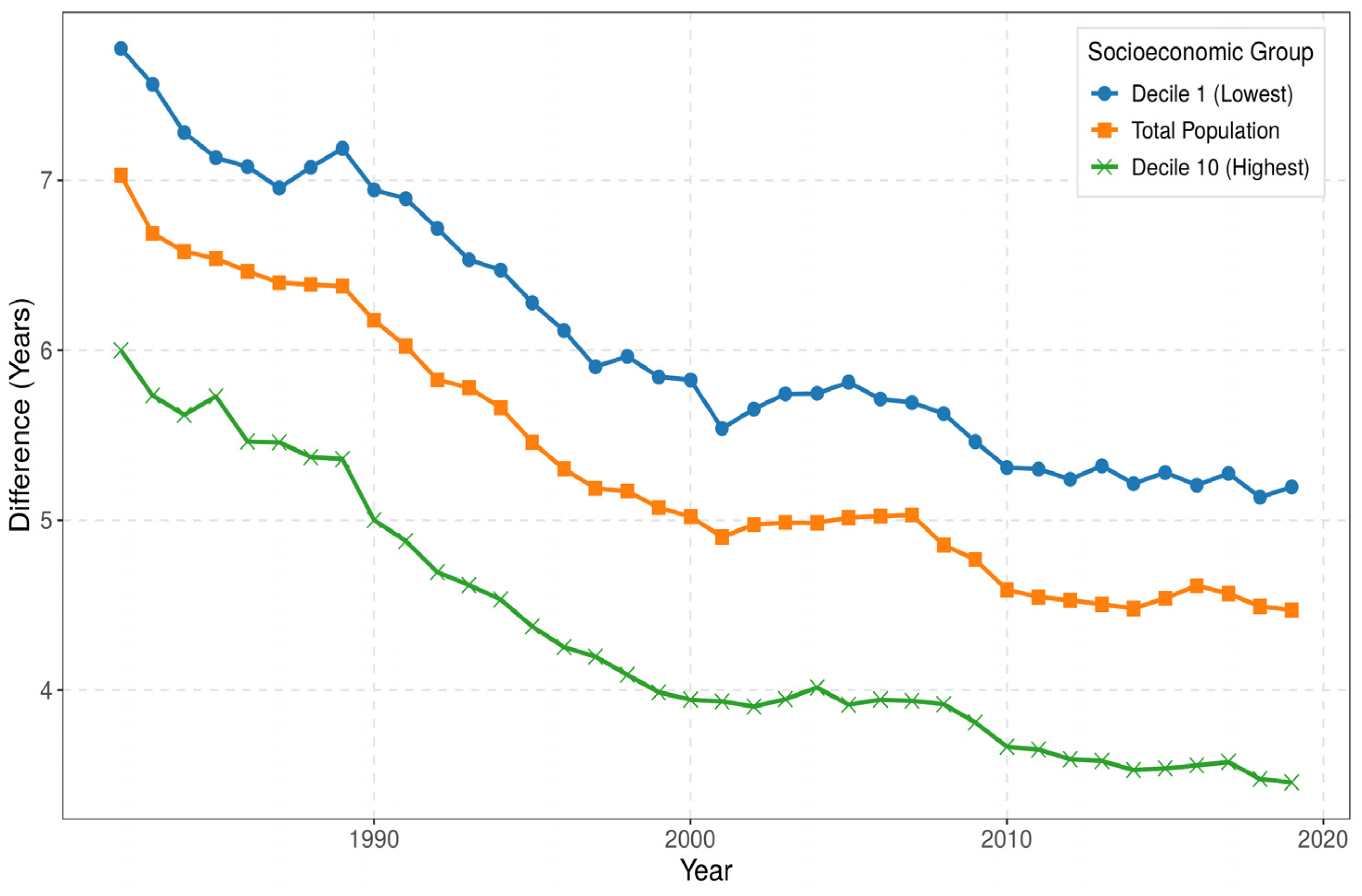
Conceptually, the Human Life Indicator (HLI) is life expectancy at birth adjusted for the inequality in the age pattern of deaths. The difference between life expectancy at birth and the HLI provides a measure of that inequality. We show those differences in Figure 2. The difference between life expectancy at birth and the HLI tends to decrease over time for all the deciles, indicating increasing mortality compression. The differences between the first and tenth declines remained roughly constant. There was essentially little change over time in the inequality in lifespan variation across the socioeconomic groups.

3.2. The Divergence in Mortality at Older Ages

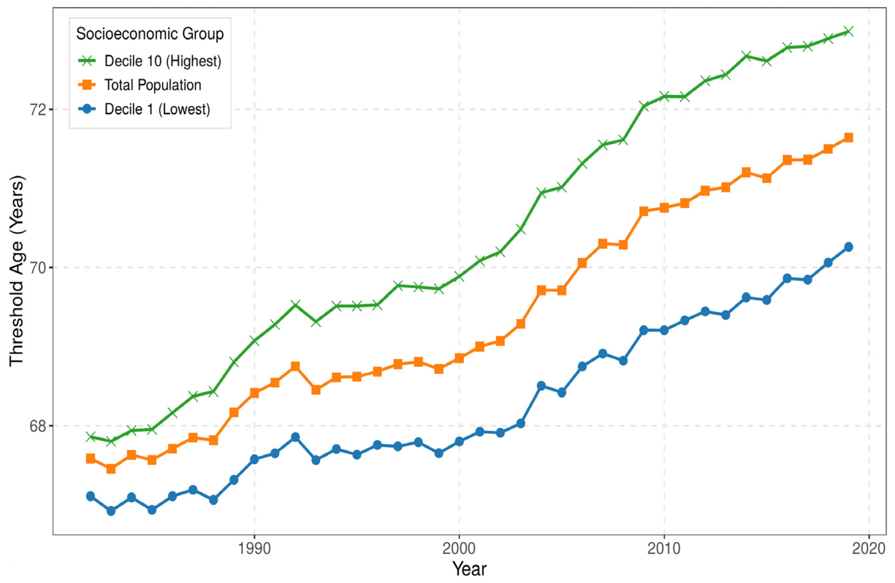
We use the POAT to assess inequality in mortality conditions at older ages. In previous work, we have shown that the POAT can be used as a temporally and spatially consistent threshold that distinguishes “older adults” from younger ones [5]. Figure 3 shows the evolution of the POATs. Over time, the POATs show increasing inequality. This divergence is almost completely accounted for by changes from 1982 to 2010. POATs increased from 2010 to 2019, but without any notable further divergence.

3.3. The Divergence in Mortality in Midlife

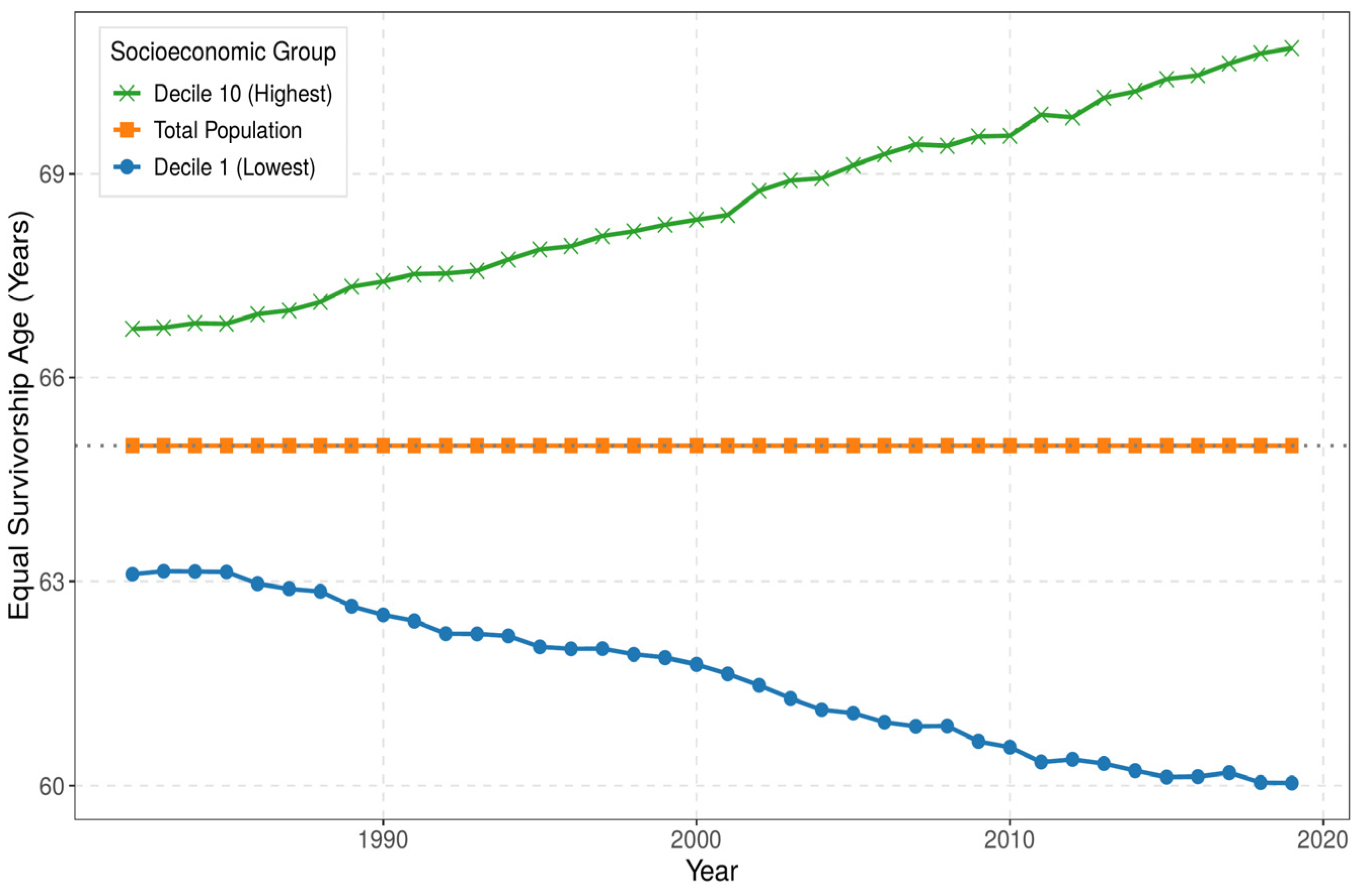
We present ESAs in Figure 4, and use them to assess the divergence of survival rates in midlife. The ESA is a detrended measure so that stable inequality would appear as parallel lines in that Figure. Instead, the lines diverge relatively consistently, without any clear change in the 2010–2019 period. Figure 4 presents a picture of a persistent growth of inequality that has little year-to-year variation.
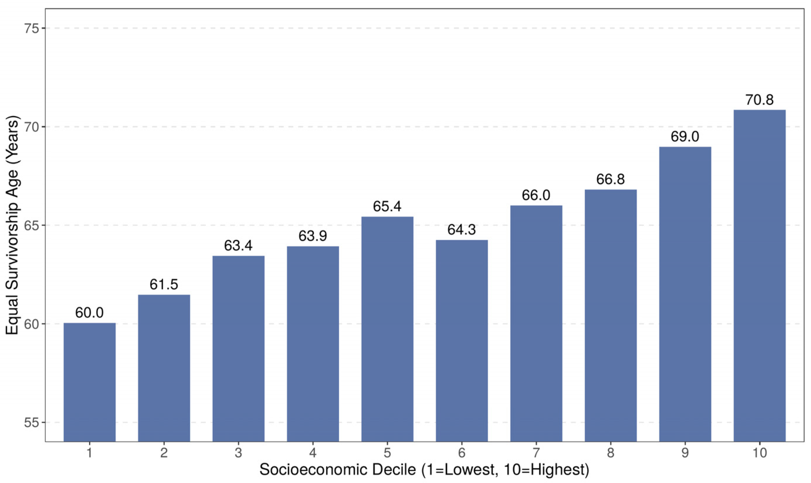
Figure 5 shows the ESA for all ten deciles in 2019. People at all the ages had the same probability of surviving from age 20. For example, people in decile 1 had the same probability of surviving from age 20 to age 60.0 as people in decile 10 had of surviving from age 20 to age 70.8.

4. Discussion

4.1. Policy Implications: The Regressivity of Retirement

The Social Security reform in the US that resulted in the increase in the normal pension age from 65 to 67 occurred in 1983 [24]. The ESA shows much smaller disparities across the socioeconomic deciles in that year. With the records and demographic methods at that time, it would have been difficult to predict what would happen. Now, the almost 11-year gap in the Equal Survivorship Age (ESA) exposes the increasingly regressive nature of raising the federal retirement age. Current proposals to increase the eligibility age are often justified by the “average” increase in life expectancy. However, our data show that raising the chronological threshold disproportionately penalizes low-SES workers who have already exhausted their survival reserves well before reaching the current cutoff.

4.2. Clinical Implications: Social-Determinant-Adjusted Geriatrics

The POAT data suggest that the onset of “old age” (defined by remaining years of life) occurs nearly 3 years earlier for those in the lowest decile compared to those in the highest (70.3 vs. 73.0 for both sexes combined). This suggests that it could be helpful to screen for geriatric syndromes (falls, dementia, sarcopenia) at an earlier age for more disadvantaged patients, rather than using fixed chronological ages to guide screening procedures.

4.3. Research Implications: Modeling Persistently Growing Inequality in Midlife

The ESA shows persistent increases in survival in the midlife. Explanations of this persistence must include factors where inequality also persistently increases. Education and income are factors commonly associated with longevity. This does not necessarily mean that education and income are factors associated with regularly increasing survival inequality seen in midlife. Income inequality does not change smoothly from year to year. The effects of the dot-com bust in 2000–2002 and the Great Recession in 2008–2009 are barely visible in the ESA figures. It is also unclear what role education plays in the persistent increases in the ESAs.
The persistent and comparatively regular increases in the ESAs favor considering cohort-based explanations such as Case and Deaton’s cumulative disadvantage hypothesis or Geronimus’ weathering hypothesis. Both of these require thinking about the determinants of survival differences in a dynamic context, and this requires new modeling that goes beyond studying the influences on survival rates at a moment in time.

4.4. Limitations of Ecological Correlations

Our analysis indicates growing inequality in survival by socio-economic decile, especially at midlife. The use of ecological correlation does not diminish the substantive importance of the large and persistent survivorship differentials documented in the paper. The results do support the conclusion that fixed chronological thresholds can mask major heterogeneity in mortality conditions across socioeconomic strata. What they do not support is a direct translation of these mortality patterns into individualized clinical or biological thresholds.

5. Conclusions

The United States is not aging as a single unit. While the wealthy enjoy a “longevity revolution” characterized by delayed aging and high survival certainty, the poor face a “longevity stagnation.” The introduction of the Equal Survivorship Age (ESA) clarifies this disparity: the poorest Americans are effectively running a longer race with a shorter timeline. To achieve health equity, we must move beyond the “myth of the average” and adopt flexible, prospective age thresholds in both clinical practice and social policy.
The object of this paper is to introduce the Equal Survivorship Age and demonstrate its usefulness in the analysis of survival inequality in combination with the HLI and the POAT. For clarity, we did not discuss gender differences here. Those differences are important for public policy, and the use of the Equal Survivorship Age to analyze them should be considered a priority. A full sex-specific presentation would have substantially expanded the scope of the manuscript and would have moved it toward a broader descriptive decomposition of mortality inequality rather than the more focused objective pursued here. We therefore chose not to add a full set of sex-specific figures in the present version.

Author Contributions

Conceptualization, W.S. and S.S.; methodology, W.S. and S.S.; software, W.S. and S.S.; validation, W.S. and S.S.; formal analysis, W.S. and S.S.; data curation, W.S. and S.S.; writing—original draft preparation, W.S. and S.S.; writing—review and editing, W.S. and S.S.; visualization, W.S. and S.S. All authors have read and agreed to the published version of the manuscript.

Funding

This research received no external funding.

Institutional Review Board Statement

Not applicable.

Informed Consent Statement

Not applicable.

Data Availability Statement

The data used in this study can be found at https://www.soa.org/resources/research-reports/2020/us-mort-rate-socioeconomic/ (accessed on 6 October 2025). Graphs were produced using Microsoft Excel.

Acknowledgments

The authors have reviewed and edited the output and take full responsibility for the content of this publication.

Conflicts of Interest

The authors declare no conflicts of interest.

Abbreviations

The following abbreviations are used in this manuscript:
HLIHuman Life Indicator
POATProspective Old Age Threshold
ESAEqual Survivorship Age
CACharacteristics Approach to the Study of Population Aging

References

  1. Chetty, R.; Stepner, M.; Lin, S.; Scuderi, B.; Turner, N.; Bergeron, A.; Cutler, D. The Association Between Income and Life Expectancy in the United States, 2001–2014. JAMA 2016, 315, 1750–1766. [Google Scholar] [CrossRef] [Scilit] [PubMed]
  2. Dwyer-Lindgren, L.; Baumann, M.M.; Li, Z.; Kelly, Y.O.; Schmidt, C.; Searchinger, C.; La Motte-Kerr, W.; Bollyky, T.J.; Mokdad, A.H.; Murray, C.J.L. Ten Americas: A systematic analysis of life expectancy disparities in the USA. Lancet 2024, 404, 2299–2313. [Google Scholar] [CrossRef] [Scilit] [PubMed]
  3. Case, A.; Deaton, A. Mortality and morbidity in the 21st century. Brook. Pap. Econ. Act. 2017, 2017, 397–476. [Google Scholar] [CrossRef] [Scilit] [PubMed]
  4. Case, A.; Deaton, A. The Great Divide: Education, Despair, and Death. Annu. Rev. Econ. 2022, 14, 1–21. [Google Scholar] [CrossRef] [Scilit] [PubMed]
  5. Sanderson, W.C.; Scherbov, S. Prospective Longevity: A New Vision of Population Aging; Harvard University Press: Cambridge, MA, USA, 2019. [Google Scholar]
  6. Eames, M.; Ben-Shlomo, Y.; Marmot, M.G. Social deprivation and premature mortality: Regional comparison across England. Br. Med. J. 1993, 307, 1097–1102. [Google Scholar] [CrossRef] [Scilit] [PubMed]
  7. Carstairs, V.; Morris, R. Deprivation: Explaining differences in mortality between Scotland and England and Wales. Br. Med. J. 1989, 299, 886–889. [Google Scholar] [CrossRef] [Scilit] [PubMed]
  8. Singh, G.K.; Siahpush, M. Widening socioeconomic inequalities in US life expectancy, 1980–2000. Int. J. Epidemiol. 2006, 35, 969–979. [Google Scholar] [CrossRef] [Scilit] [PubMed]
  9. Singh, G.K.; Siahpush, M. Widening Rural–Urban Disparities in Life Expectancy, U.S., 1969–2009. Am. J. Prev. Med. 2014, 46, e19–e29. [Google Scholar] [CrossRef] [Scilit] [PubMed]
  10. Dwyer-Lindgren, L.; Bertozzi-Villa, A.; Stubbs, R.W.; Morozoff, C.; Mackenbach, J.P.; van Lenthe, F.J.; Mokdad, A.H.; Murray, C.J.L. Inequalities in Life Expectancy Among US Counties, 1980 to 2014: Temporal Trends and Key Drivers. JAMA Intern. Med. 2017, 177, 1003–1011. [Google Scholar] [CrossRef] [Scilit] [PubMed]
  11. Case, A.; Deaton, A. Rising morbidity and mortality in midlife among white non-Hispanic Americans in the 21st century. Proc. Natl. Acad. Sci. USA 2015, 112, 15078–15083. [Google Scholar] [CrossRef] [Scilit] [PubMed]
  12. Geronimus, A.T.; Hicken, M.; Keene, D.; Bound, J. ‘Weathering’ and Age Patterns of Allostatic Load Scores Among Blacks and Whites in the United States. Am. J. Public Health 2006, 96, 826–833. [Google Scholar] [CrossRef] [Scilit] [PubMed]
  13. Geronimus, A.T.; Bound, J.; Waidmann, T.A.; Rodriguez, J.M.; Timpe, B. Weathering, Drugs, and Whack-a-Mole: Fundamental and Proximate Causes of Widening Educational Inequity in U.S. Life Expectancy by Sex and Race, 1990–2015. J. Health Soc. Behav. 2019, 60, 222–239. [Google Scholar] [CrossRef] [Scilit] [PubMed]
  14. Crimmins, E.M.; Beltrán-Sánchez, H. Mortality and morbidity trends: Is there compression of morbidity? J. Gerontol. B Psychol. Sci. Soc. Sci. 2011, 66B, 75–86. [Google Scholar] [CrossRef] [Scilit] [PubMed]
  15. Ghislandi, S.; Sanderson, W.C.; Scherbov, S. A simple measure of human development: The Human Life Indicator. Popul. Dev. Rev. 2019, 45, 219–233. [Google Scholar] [CrossRef] [Scilit] [PubMed]
  16. van Raalte, A.A.; Sasson, I.; Martikainen, P. The case for monitoring life-span inequality. Science 2018, 362, 1002–1004. [Google Scholar] [CrossRef] [Scilit] [PubMed]
  17. Sasson, I. Trends in Life Expectancy and Lifespan Variation by Educational Attainment: United States, 1990–2010. Demography 2016, 53, 269–293. [Google Scholar] [CrossRef] [Scilit] [PubMed]
  18. WHO. World Report on Ageing and Health 2015; World Health Organization: Geneva, Switzerland, 2015. [Google Scholar]
  19. Sanderson, W.C.; Scherbov, S. The characteristics approach to the measurement of population aging. Popul. Dev. Rev. 2013, 39, 673–685. [Google Scholar] [CrossRef] [Scilit]
  20. Sanderson, W.C.; Scherbov, S. Measuring the speed of aging across population subgroups. PLoS ONE 2014, 9, e96289. [Google Scholar] [CrossRef] [Scilit]
  21. Sanderson, W.C.; Scherbov, S. Average remaining lifetimes can increase as human populations age. Nature 2005, 435, 811–813. [Google Scholar] [CrossRef] [Scilit] [PubMed]
  22. Barbieri, M. Socioeconomic Disparities Do Not Explain the U.S. International Disadvantage in Mortality. J. Gerontol. Ser. B 2022, 77, S158–S166. [Google Scholar] [CrossRef] [Scilit] [PubMed]
  23. Barbieri, M. Mortality by Socioeconomic Category in the United States; Society of Actuaries: Schaumburg, IL, USA, 2020. [Google Scholar]
  24. Social Security History. Social Security. Available online: https://www.ssa.gov/history/1983amend.html (accessed on 25 January 2026).
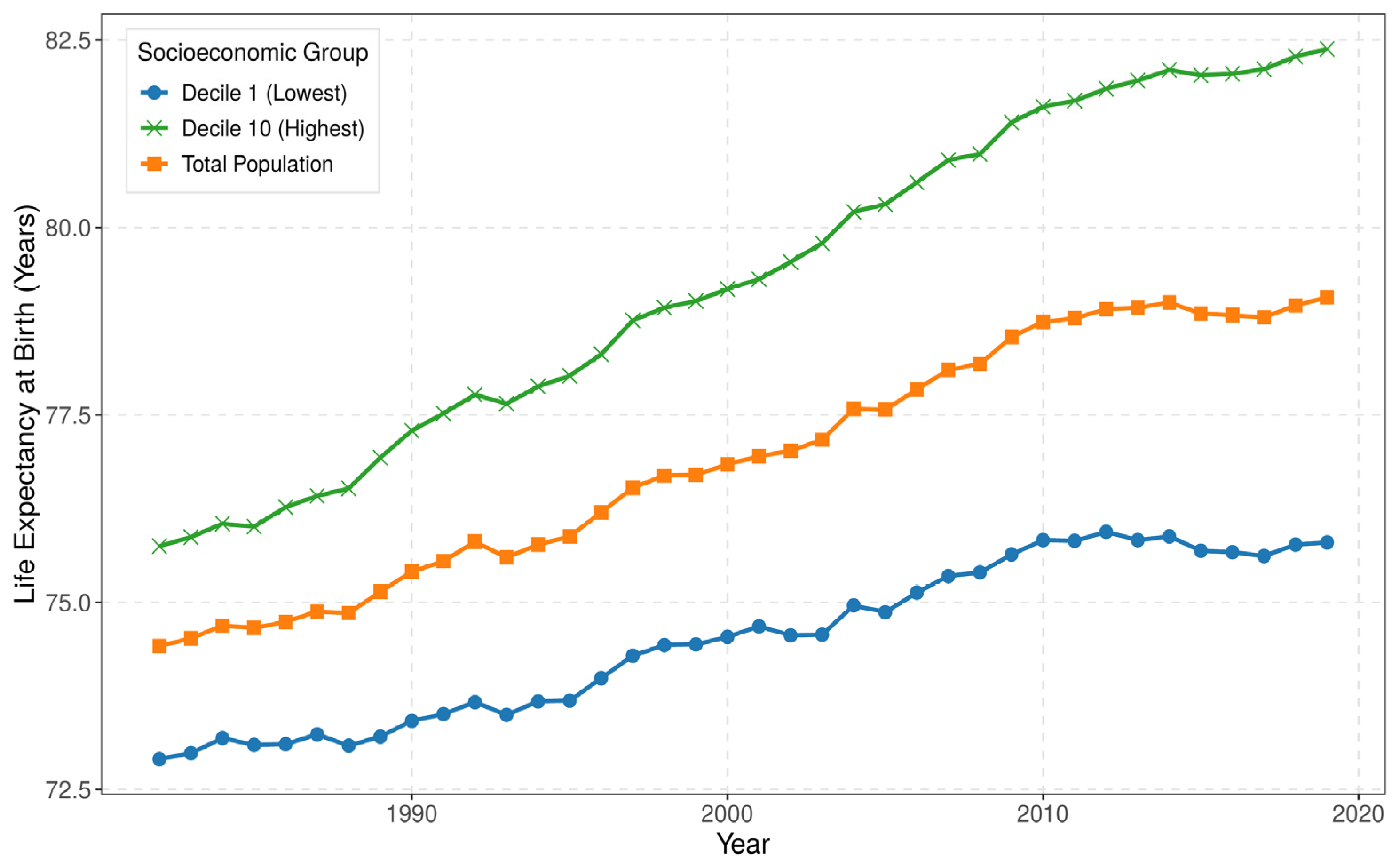
Figure 1. Trends in Life Expectancy at Birth by Socioeconomic Decile (1982–2019). This figure illustrates the “Great Divergence” in longevity between the highest socioeconomic decile (Decile 10), the lowest decile (Decile 1), and the total U.S. population. While the national average and the top decile show significant gains in life expectancy over nearly four decades, the bottom decile exhibits relative stagnation, resulting in a gap between the deciles that widened from 2.8 years in 1982 to 6.6 years by 2019.
Tph 01 00003 g001
Figure 2. Temporal Trends in Longevity Inequality (life expectancy at birth minus HLI) (1982–2019). Longevity inequality is measured here as the difference between life expectancy at birth (e0) and the Human Life Indicator (HLI). The Figure shows little change in inequality over time.
Tph 01 00003 g002
Figure 3. Evolution of the Prospective Old-Age Threshold (POAT) by Socioeconomic Status (1982–2019). Following the Sanderson–Scherbov framework, the POAT represents the age at which remaining life expectancy is exactly 15 years. This chart shows the increase in the inequality in that threshold prior to 2010.
Tph 01 00003 g003
Figure 4. Divergence of the Equal Survivorship Age (ESA) from the National Benchmark (1982–2019). This figure tracks the ESA over time, using the total population survival probability to age 65 as a fixed benchmark (represented by the horizontal “Total Population” line at 65.0). The chart highlights a critical social divergence: since 1982, the highest decile has gained nearly four years of survival parity, while the lowest decile has seen its survival parity regress from age 63 to age 60.
Tph 01 00003 g004
Figure 5. Gradient of the Equal Survivorship Age (ESA) Across Socioeconomic Deciles (2019). The bar chart displays the ESA for each decile, representing the chronological age at which that group reaches the same survival probability (from age 20) as the national average at age 65. The nearly 11-year gap between Decile 1 (60.0 years) and Decile 10 (70.8 years) demonstrates that individuals in the lowest socioeconomic strata exhaust their survival reserves more than a decade earlier than those in the highest strata.
Tph 01 00003 g005
Disclaimer/Publisher’s Note: The statements, opinions and data contained in all publications are solely those of the individual author(s) and contributor(s) and not of MDPI and/or the editor(s). MDPI and/or the editor(s) disclaim responsibility for any injury to people or property resulting from any ideas, methods, instructions or products referred to in the content.