Modeling Glucocorticoid-Induced Renin Regulation from Sparse Data Using Physics-Informed Neural Networks

Abstract

Glucocorticoid-induced hypertension affects over 30% of treated patients, yet its underlying mechanisms remain unclear, particularly how glucocorticoids regulate renin within the renin-angiotensin-aldosterone system (RAAS). Modeling these dynamics is difficult because only four dose-response measurements are available at a single 24-h timepoint (36 observations total), while the system depends on roughly eleven biochemical parameters spanning minutes-long receptor interactions to days-long protein secretion. Classical parameter estimation becomes unreliable in this extremely underdetermined setting, and purely data-driven methods offer limited biological interpretability. In this paper, we introduce a physics-informed neural network (PINN) framework that integrates ELISA measurements from As4.1 juxtaglomerular cells, ordinary differential equations describing glucocorticoid receptor signaling and renin transcription, and automatic differentiation to enforce mechanistic constraints. By systematically tuning synthetic-data weights (SW in {0.2, 0.3, 0.5}), we identify an intermediate value of SW = 0.3 that provides the best overall balance between predictive accuracy, accepted ensemble size, and biologically plausible parameter estimates among the tested configurations. The framework uses adaptive constraint scheduling with a plateau ramp to reduce premature convergence and introduces calibrated plausibility thresholds reflecting experimental noise. The accepted PINN ensemble (n = 5, 50% success rate) achieved R² = 0.803, compared with 0.759 for the SW = 0.5 baseline and −0.220 for the ODE-only baseline, with RMSE = 0.024. Key learned parameters (IC₅₀ = 2.925 ± 0.012 mg/dL, Hill = 1.950 ± 0.009) are biologically plausible within the model assumptions, and the best single accepted model attained R² = 0.891. Information criteria favored the PINN over the ODE model, with improvements of approximately 77× (AIC) and 5.9× (BIC). Despite training on a single timepoint, the PINN also infers full 48-h trajectories and reproduces non-monotonic dose-response behavior. This work presents, to our knowledge, the first PINN framework for glucocorticoid-mediated renin regulation and should be interpreted as a proof-of-concept approach for integrating sparse biomedical data with mechanistic constraints. The inferred parameters and temporal dynamics are best viewed as model-dependent, hypothesis-generating estimates rather than validated biological quantities.

1. Introduction

Glucocorticoid therapy, widely prescribed for autoimmune disorders, transplantation, and critical illness, paradoxically induces hypertension in over 30% of patients [1,2]. This is particularly puzzling for synthetic glucocorticoids like dexamethasone, which exhibit negligible mineralocorticoid effects yet still cause blood pressure elevation [3]. Recent evidence reveals complex, tissue-specific effects: while systemic RAAS is typically suppressed by glucocorticoid excess (as seen in Cushing’s syndrome with low plasma renin [4]), local tissue RAAS may paradoxically increase in adipose tissue and correlate with blood pressure elevation, and prenatal glucocorticoid exposure can program lifelong upregulation of renin, ACE, and AT₁ receptor expression in offspring [5]. Additionally, glucocorticoids suppress ACE2 expression in pancreatic tissue, disrupting the protective arm of the RAAS cascade [6]. Understanding this paradox requires investigating the RAAS, the master regulator of blood pressure homeostasis, where renin serves as the rate-limiting enzyme initiating the cascade to angiotensin II production and sodium retention [7].

The recent experimental work seen in [8] represents the first systematic in vitro investigation of glucocorticoid effects on renin expression, in an As4.1 cell model. Earlier studies had observed glucocorticoid-mediated changes in renin in vivo, but not with a comparable dose-response approach [9,10,11]. Using ELISA measurements at 24 h across four concentrations (0, 0.3, 3.0, 30.0 mg/dL), it was demonstrated in [8] a statistically significant, dose-dependent suppression with median renin decreasing from 28.1 ng/mL (control) to 25.7, 23.8, and 25.7 ng/mL, respectively (p < 0.05 for all comparisons). The non-monotonic response at the highest dose suggests complex regulatory mechanisms, including potential receptor saturation. However, critical questions remained regarding kinetic parameters, temporal dynamics beyond 24 h, rate-limiting mechanisms, and prediction capabilities for untested conditions.

The experimental data present formidable modeling challenges: only 4 dose points with 9 ELISA replicates each (36 total observations) at a single timepoint, yet the biological system involves at least 6 state variables (free/bound glucocorticoid receptors, cytoplasmic/nuclear complexes, renin mRNA, protein, secreted) governed by approximately 11 biochemical parameters (binding kinetics, translocation rates, transcription/translation/degradation rates, IC₅₀, Hill coefficient). This severe parameter-to-data ratio (~0.31) violates standard estimation requirements. Moreover, the system spans multiple timescales from receptor binding (seconds-minutes) to transcription (hours) and protein secretion (hours-days), yet observations collapse to one 24-h snapshot.

Traditional ODE fitting becomes unreliable in this setting: with 36 observations and 11 parameters, multiple parameter sets can produce near-identical fits while implying substantially different biological interpretations [12,13]. The corresponding loss landscapes may exhibit flat regions, multiple local minima, and ill-conditioning, which further complicate parameter estimation [14]. Standard least-squares approaches provide point estimates without directly addressing parameter uncertainty, while Bayesian methods face substantial computational and identifiability challenges in such sparse-data regimes [15,16]. Pure machine-learning alternatives can fit the available observations, but they are prone to overfitting, do not enforce biological constraints (e.g., non-negative concentrations), and cannot reliably infer time-courses from single-timepoint data alone [17].

PINNs, pioneered by the authors in [18], embed mechanistic knowledge directly into neural network training through unified optimization. Recent comprehensive reviews have systematically analyzed PINN developments, with the authors in [19] establishing a three-dimensional analytical framework showing 230% convergence acceleration in Navier-Stokes solutions through adaptive optimization and 72% cost reduction compared to FEM in high-dimensional spaces. Rather than treating differential equations and data separately, PINNs minimize composite loss functions simultaneously enforcing: (1) data fidelity through squared errors against measurements, (2) physical law compliance via ODE residuals computed through automatic differentiation, and (3) initial condition satisfaction [20].

The key innovation replaces expensive numerical ODE solvers with automatic differentiation, enabling enforcement of physical constraints at thousands of collocation points without explicitly solving equations [21]. Unknown biochemical parameters are jointly optimized with network weights, ensuring only dynamically consistent solutions minimize the loss [22]. This addresses sparse data through physics-based inductive bias, temporal information propagation from single timepoints, and built-in uncertainty quantification via Monte Carlo dropout [23,24]. Recent applications have successfully tackled biological systems with similar data sparsity, including epidemiological models achieving robust parameter estimation from limited observations [25], physiological signal processing from scarce clinical data [26], and chemical reaction networks with automatic model reduction [27].

Therefore, the glucocorticoid-renin system is ideal for PINN methodology due to well-characterized biochemistry providing strong prior knowledge, sparse yet high-quality multi-scale data enabling constraint at multiple biological scales, and immediate clinical relevance for personalized hypertension risk prediction and therapeutic dosing optimization.

This work makes three main contributions:

• We present a PINN framework for modeling glucocorticoid-mediated renin regulation from extremely sparse data by integrating 24-h ELISA measurements with a mechanistic ODE system. Across the tested synthetic-data weights (SW in {0.2, 0.3, 0.5}), the intermediate configuration SW = 0.3 provided the best overall balance among the tested settings. The accepted ensemble (n = 5, 50% success rate) achieved R² = 0.803, compared with R² = 0.759 for the conventional PINN baseline and R² = −0.220 for the ODE-only baseline, with RMSE = 0.024. Information criteria also favored the PINN over the ODE baseline by factors of 77× (AIC) and 5.9× (BIC).
• We show that joint optimization of approximately 50,000 network weights and 11 biochemical parameters yields biologically plausible parameter estimates and enables inference of model-consistent temporal trajectories from single-timepoint data. The accepted ensemble produced IC₅₀ = 2.925 ± 0.012 mg/dL and Hill coefficient = 1.950 ± 0.009, while also reproducing the experimentally observed non-monotonic high-dose response.
• We provide a transparent evaluation of the framework under severe data scarcity through comparisons across PINN configurations, benchmarking against ODE-only and pure neural-network baselines, and additional validation analyses. These include residual analysis, leave-one-dose-out (LODO) evaluation, deterministic ensemble assessment, and explicit discussion of limitations such as weak identifiability and unstable global sensitivity analysis. Together, these results position the framework as a proof-of-concept methodology for sparse biomedical modeling rather than a definitive biological model.

The paper is organized as follows. Section 2 reviews the biological and computational background relevant to glucocorticoid-mediated renin regulation, including RAAS physiology, glucocorticoid signaling, experimental findings, and physics-informed modeling foundations. Section 3 presents the proposed framework, including the ODE system, neural-network architecture, loss formulation, and training methodology. Section 4 reports the main experimental results, including parameter estimates, dose-response behavior, temporal trajectories, and comparative evaluation against baseline approaches. Section 5 discusses biological interpretation, uncertainty, limitations, and broader implications of the framework. Section 6 concludes the study and outlines future directions.

2. State-of-the-Art

This section summarizes the biological and computational background relevant to glucocorticoid-mediated renin regulation, including RAAS physiology, glucocorticoid signaling, the experimental foundation of the present study, traditional computational approaches, and PINNs.

2.1. The RAAS

The RAAS [28] is one of the best-studied endocrine cascades in physiology, originally described by the authors in [29], and remains clinically central to the treatment of hypertension, heart failure, and chronic kidney disease. The cascade begins with renin, an aspartyl protease synthesized by specialized juxtaglomerular cells in renal afferent arterioles. In response to decreased perfusion pressure, reduced macula densa sodium delivery, or beta1-adrenergic stimulation, these cells release renin into circulation, where it cleaves hepatic angiotensinogen to generate angiotensin I. Angiotensin-converting enzyme (ACE) subsequently converts angiotensin I to angiotensin II, a potent vasoconstrictor that raises blood pressure directly and indirectly through aldosterone-mediated sodium retention [30].

The clinical importance of the RAAS is underscored by the widespread use of ACE inhibitors, angiotensin receptor blockers (ARBs), and direct renin inhibitors [31]. Beyond the classical systemic pathway, accumulating evidence indicates the existence of tissue-specific RAAS systems. The authors in [7] reviewed multiple organs expressing complete or partial RAAS components capable of local angiotensin II generation. In Cushing’s syndrome, adipose tissue has been shown to exhibit increased renin gene expression and protein levels despite suppressed circulating renin, with adipose renin correlating significantly with blood pressure [4]. In addition, developmental programming studies demonstrate that prenatal dexamethasone exposure can upregulate renin, prorenin receptor, ACE, and AT1R expression in adult offspring, contributing to later hypertension [5]. These findings highlight the complexity of glucocorticoid-RAAS interactions beyond the classical systemic cascade. At the transcriptional level, the mouse Ren-1c promoter contains multiple mapped transcription factor binding sites, with the proximal promoter region (~200 bp upstream) showing basal activity through critical HOX-PBX sites at positions −72 to −50 that are essential for cell-type specificity [32].

RAAS complexity also extends to alternative processing pathways. Angiotensin-converting enzyme 2 (ACE2), identified by the authors in [33], cleaves angiotensin II to generate angiotensin-(1-7), which acts through the Mas receptor and exerts vasodilatory and anti-fibrotic effects that oppose angiotensin II. The balance between the ACE/Ang II axis and the ACE2/Ang-(1-7)/Mas axis is therefore important for hypertension pathophysiology [34].

2.2. Glucocorticoid Signaling Mechanisms

Glucocorticoids are steroid hormones synthesized in the adrenal cortex zona fasciculata and regulate metabolism, immunity, stress responses, and development. Endogenous cortisol follows circadian secretion patterns controlled by hypothalamic corticotropin-releasing hormone and pituitary adrenocorticotropic hormone. Synthetic glucocorticoids such as dexamethasone exhibit substantially greater potency than cortisol, essentially no mineralocorticoid activity, and longer half-life [35,36].

At the molecular level, glucocorticoids diffuse across the plasma membrane and bind cytoplasmic glucocorticoid receptors (GR, encoded by NR3C1), members of the nuclear receptor superfamily that reside in complexes with heat shock proteins [37]. Ligand binding induces conformational changes, chaperone dissociation, exposure of nuclear localization signals, and active nuclear transport. Nuclear ligand-bound GR predominantly homodimerizes and binds glucocorticoid response elements (GREs), typically palindromic sequences in promoter or enhancer regions [38].

Clinically, recent guidelines from the European Society of Endocrinology and the Endocrine Society indicate that glucocorticoid doses exceeding daily hydrocortisone equivalents of 15–25 mg may pose a risk for adrenal insufficiency, underscoring the narrow therapeutic window [1]. Glucocorticoid-induced adrenal insufficiency can occur with any formulation, with no firmly established safe threshold [2]. At the same time, the mechanisms underlying glucocorticoid-induced hypertension remain incompletely understood, particularly for synthetic glucocorticoids with minimal mineralocorticoid activity [3]. Recent studies further suggest that dexamethasone can suppress ACE2 expression in pancreatic beta-cells, thereby impairing the protective ACE2/Ang-(1-7)/Mas axis [6]. In inflammatory settings such as sepsis, dexamethasone markedly reduces Ang II levels in plasma, lung, and kidney tissues while downregulating AT2R expression [39]. Together, these findings support the view that glucocorticoids modulate the RAAS in a tissue- and context-dependent manner.

2.3. Experimental Foundation

Latia’s dissertation [8] provides the main experimental foundation for the present study and represents a systematic in vitro investigation of glucocorticoid effects on renin expression. Earlier in vivo studies had already shown that glucocorticoids can modulate renin, including chronic cortisol infusion in fetal sheep, suppressing renal renin mRNA by approximately 77% [9], maternal dexamethasone lowering plasma renin in pregnant ewes [10], and cortisol-renin dynamics being examined in teleost fish [11]. Motivated by clinical observations of hypertension with altered renin under glucocorticoid treatment, Latia [8] used As4.1 cells, a juxtaglomerular-like cell line isolated by Sigmund et al. [40] from transgenic mice expressing endogenous Ren-1c.

In that experimental design, four dexamethasone concentrations spanning three orders of magnitude were tested: 0 mg/dL (control), 0.3 mg/dL, 3.0 mg/dL, and 30.0 mg/dL. Cells were cultured in DMEM with 10% fetal calf serum at 37 degrees C and 5% CO₂ for 24-h stimulation. Mouse prorenin/renin ELISA was used to quantify secreted renin in culture supernatants. Nine replicates per condition were obtained through three independent experiments with technical triplicates. The control median was 28.1 ng/mL (IQR 26.0–28.8), decreasing to 25.7 ng/mL at 0.3 mg/dL (IQR 24.6–27.0), 23.8 ng/mL at 3.0 mg/dL (IQR 23.2–24.8), and partially recovering to 25.7 ng/mL at 30.0 mg/dL (IQR 19.7–27.7). Wilcoxon signed-rank tests showed significant suppression at all tested doses (p < 0.05).

The most notable feature of the dataset is the non-monotonic dose-response, with maximal suppression at 3.0 mg/dL and partial recovery at 30.0 mg/dL. This pattern suggests that simple monotonic inhibition may be insufficient and that receptor saturation, competing regulatory mechanisms, or altered GR sensitivity at high doses may contribute. The finding is broadly consistent with evidence that glucocorticoid effects on RAAS components depend on tissue context, developmental timing, and exposure duration [4,5]. At the same time, the dataset remains extremely sparse from a modeling perspective, with only four dose conditions measured at a single timepoint. Similar sparse-data challenges have been addressed in other biological settings using PINNs [25,26] and Bayesian approaches [15], but not specifically for the glucocorticoid-renin system.

2.4. Traditional Computational Approaches

Quantitative biochemical modeling has evolved from Michaelis-Menten kinetics to modern systems biology formulations based on coupled ordinary differential equations (ODEs), in which each species $i$ follows a rate equation ${dy}_i/dt={\mathrm{\Sigma }}_j{v}_j\left(y,\theta \right)$, where $v_j$ denotes reaction rates and theta denotes biochemical parameters [41].

Given time-series measurements, the inverse problem seeks parameters θ that minimize residuals between model predictions and observations. Recent advances include weak-form estimation methods that improve robustness to noise [12] and sparse Bayesian frameworks for discovering interpretable dynamics [42]. However, when the number of measurements $N$ is small relative to the number of parameters $p$, standard asymptotic approximations break down, and overfitting becomes severe [43]. A central issue is parameter identifiability: whether parameters can be uniquely determined from the available data. The authors in [44] showed that even moderately complex models may exhibit substantial non-identifiability under typical experimental conditions. Recent Bayesian approaches attempt to address this through sparse priors and more efficient computation, but the problem remains difficult in severely underdetermined regimes [16].

Several recent methods explicitly target sparse-data scenarios. The Weak-form Estimation of Nonlinear Dynamics (WENDy) approach estimates ODE parameters using weak-form constraints and can outperform traditional least-squares under noisy conditions [12]. Other approaches combine machine learning with mechanistic constraints to identify governing equations from limited observations [13,22], while elastic net and group lasso have been used for sparse recovery in first-order reaction systems [45]. Nevertheless, for endocrine datasets with only a few dose conditions and a single timepoint, traditional approaches remain strongly limited by identifiability and data sparsity.

2.5. PINN Foundations and Applications

PINNs arose from combining three ideas: neural networks are universal function approximators for differential equation solutions, automatic differentiation enables efficient derivative computation, and physical laws can be incorporated as soft constraints during training. The authors in [18] showed that neural networks could solve forward and inverse problems for differential equations by minimizing losses that combine data fidelity and equation residuals.

For a differential equation $Nu=f\left(x\right)$ on domain $\Omega$ with boundary conditions $Bu=g\left(x\right)$ on $\partial \Omega$, a neural network $u_{NN}\left(x;w\right)$ with parameters $w$ can approximate $u$ by minimizing a loss of the form $L_{total}=L_{data}+{\lambda }_{phisics}·L_{phisics}+{\lambda }_{BC}·L_{BC}$ [46]. Recent theoretical advances established convergence guarantees and approximation error bounds for PINNs [47], while reviews in [19,21] summarized their methodological evolution and applications. In sparse-data settings, a central challenge is balancing competing objectives in the composite loss. Physics constraints can guide learning when data are scarce, but overly restrictive weighting may reduce the success rate of solutions that satisfy both data fidelity and biological plausibility. This balance is problem-dependent and usually requires empirical calibration.

Recent methodological developments include stacked PINN architectures for multifidelity learning [20], adaptive weighting schemes for balancing loss components [48], and training strategies such as re-initialization for stiff problems [49]. PINNs have also shown promise in biological applications with limited observations. The authors in [25] developed compartmental epidemiological models, achieving robust parameter estimation from sparse data. The authors in [50] predicted 3D soft-tissue dynamics from 2D imaging, and the authors in [26] modeled physiological time series for cuffless blood pressure estimation, both showing that physics-based constraints can improve learning from limited ground truth. Related work on chemical reaction networks has demonstrated automatic model reduction while maintaining predictive accuracy [27].

Monte Carlo dropout is one practical approach for uncertainty quantification in neural models and has also been explored in PINN settings [23,24,51]. However, uncertainty quantification remains challenging in sparse-data PINNs. In particular, small ensemble sizes or single successful runs may give an overly optimistic impression of stability. This issue becomes especially important when comparing configurations with different success rates, because a single passing model may not be representative of the overall method.

2.6. Recent PINN Developments

PINN methodology has advanced rapidly in recent years. Reviews have reported improvements in convergence speed and computational efficiency through adaptive optimization and improved training strategies [19]. The authors in [52] developed physics-informed CNNs for PDEs on spheres, and trainable embedding approaches have been proposed for nonlinear PDEs in quantum systems [53]. Boundary-condition handling has also been refined, with comparisons between soft and hard enforcement strategies [54], while domain decomposition approaches such as XPINNs enable parallelization and treatment of complex geometries [55]. More broadly, the integration of PINNs with operator-learning approaches and neural operators continues to expand the range of physics-informed machine-learning methods [56].

2.7. GAP Analysis and Contributions

Important gaps remain at the intersection of RAAS biology and computational modeling. While qualitative evidence for glucocorticoid-mediated renin regulation is increasing, quantitative kinetic parameters remain poorly characterized [57]. The experimental work in [8] provides a valuable systematic dose-response dataset, but it is limited to a single 24-h timepoint with few effective conditions for model calibration. Existing biological PINN applications have generally focused on systems with richer validation data, while some recent sparse-data biological applications rely on image-based spatial densities rather than the discrete low-n measurements typical of endocrine assays [58]. To our knowledge, neither joint learning of ODE dynamics and biochemical parameters from this type of sparse glucocorticoid-renin dataset nor systematic calibration of physics-informed constraints in such an underdetermined setting has been demonstrated [48].

Recent physics-informed approaches have begun addressing sparse-data challenges through multi-objective optimization [59], but the balance between data fidelity and physics compliance remains problem-dependent [60]. Stronger constraints can guide learning, yet they may also reduce the number of solutions that remain both numerically stable and biologically plausible. In addition, ensemble size requirements for statistically meaningful comparison remain insufficiently discussed in sparse-data PINN studies [61]. These issues motivate the present work.

Accordingly, the aim of this study is not to claim definitive biological identification from limited data, but to evaluate whether a physics-informed framework can provide more stable and biologically plausible estimates than ODE-only fitting or unconstrained learning in a severely data-limited setting. The present work, therefore, focuses on integrating sparse experimental measurements with a mechanistic ODE model, calibrating the relative strength of data and physics constraints, and assessing variability across accepted model runs under explicit identifiability limitations.

3. Proposed Framework

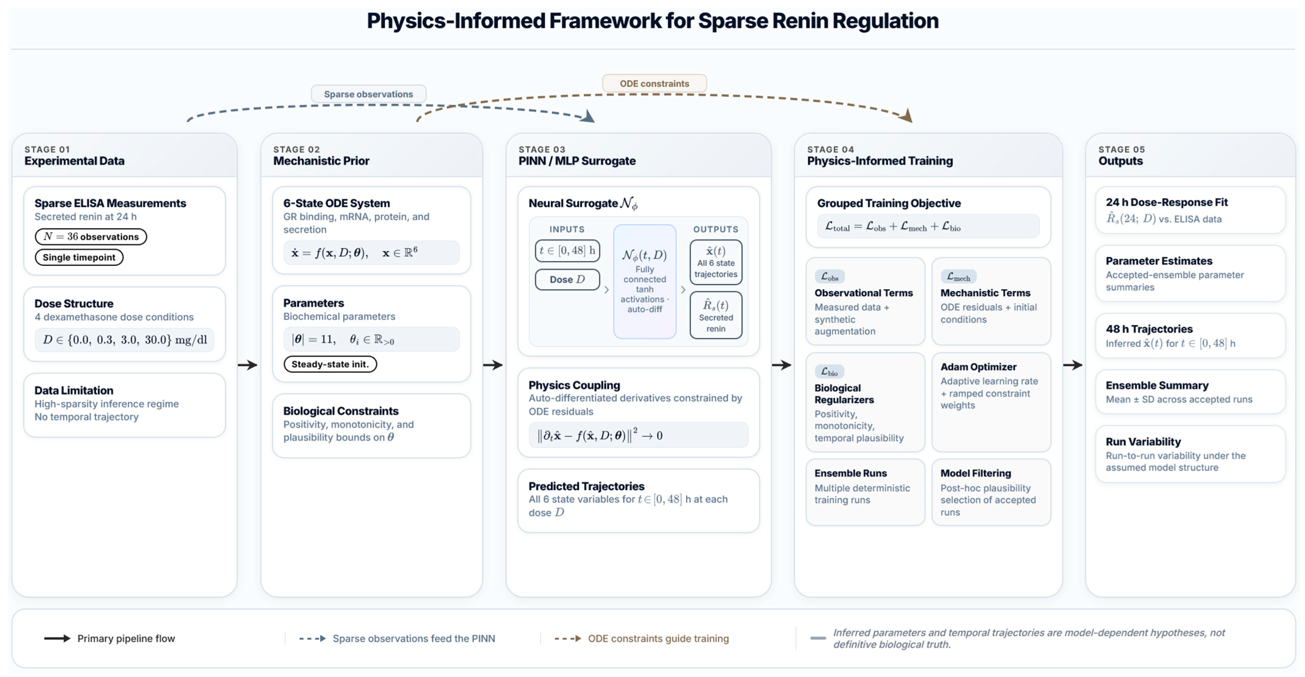
This section presents our PINN framework for modeling glucocorticoid regulation of renin from sparse experimental data. The framework integrates mechanistic ordinary differential equations capturing receptor dynamics and gene regulation with neural network function approximation and automatic differentiation for parameter learning. To clarify the overall workflow of the proposed approach, Figure 1 summarizes how sparse experimental measurements, mechanistic ODE constraints, and the neural surrogate are integrated during training to produce dose-response predictions, parameter estimates, and inferred temporal trajectories.

3.1. ODE System Formulation

The biological system involves glucocorticoid receptor activation and subsequent renin gene regulation spanning multiple molecular processes and timescales. We formulate a six-state ODE system capturing these dynamics with state variables representing free cytoplasmic glucocorticoid receptor concentration ${\mathrm{GR}}_{\mathrm{free}}$, cytoplasmic GR-ligand complex concentration ${\mathrm{GR}}_{\mathrm{cyto}}$, nuclear GR-ligand complex concentration ${\mathrm{GR}}_{\mathrm{nuc}}$, renin mRNA concentration $\mathrm{mRNA}$, intracellular renin protein concentration $\mathrm{Protein}$, and extracellular secreted renin concentration $\mathrm{Secreted}$.

The glucocorticoid receptor dynamics follow ligand binding, nuclear translocation, and turnover according to Equations (1)–(3) [62,63,64,65]:

$$\begin{array}{c}{\displaystyle \frac{d\left[{\mathrm{GR}}_{\mathrm{free}}\right]}{dt}}=k_{\mathrm{synth},\mathrm{GR}}-k_{\mathrm{deg},\mathrm{GR}}\left[{\mathrm{GR}}_{\mathrm{free}}\right]\\ -k_{\mathrm{bind}}\left[{\mathrm{GR}}_{\mathrm{free}}\right]\left[\mathrm{Dex}\right]+k_{\mathrm{unbind}}\left[{\mathrm{GR}}_{\mathrm{cyto}}\right]\end{array}$$

(1)

where $k_{\mathrm{synth},\mathrm{GR}}$ is the glucocorticoid receptor synthesis rate (${\mathrm{h}}^{-1}$), $k_{\mathrm{deg},\mathrm{GR}}$ is the receptor degradation rate (${\mathrm{h}}^{-1}$), $k_{\mathrm{bind}}$ is the GR-dexamethasone binding rate (${\mathrm{h}}^{-1}$ ${\mathrm{m}\mathrm{g}}^{-1}$ dL), $\left[\mathrm{Dex}\right]$ is the dexamethasone concentration (mg/dL), and $k_{\mathrm{unbind}}$ is the dissociation rate (${\mathrm{h}}^{-1}$).

$$\begin{array}{c}{\displaystyle \frac{d\left[{\mathrm{GR}}_{\mathrm{cyto}}\right]}{dt}}=k_{\mathrm{bind}}\left[{\mathrm{GR}}_{\mathrm{free}}\right]\left[\mathrm{Dex}\right]\\ -k_{\mathrm{unbind}}\left[{\mathrm{GR}}_{\mathrm{cyto}}\right]-k_{\mathrm{nuclear}}\left[{\mathrm{GR}}_{\mathrm{cyto}}\right]\end{array}$$

(2)

where $k_{\mathrm{nuclear}}$ is the nuclear translocation rate (${\mathrm{h}}^{-1}$) governing transport of cytoplasmic GR-ligand complexes into the nucleus through active nuclear pore transport.

$${\displaystyle \frac{d\left[{\mathrm{GR}}_{\mathrm{nuc}}\right]}{dt}}=k_{\mathrm{nuclear}}\left[{\mathrm{GR}}_{\mathrm{cyto}}\right]-k_{\mathrm{deg},\mathrm{GR}}\left[{\mathrm{GR}}_{\mathrm{nuc}}\right]$$

(3)

where nuclear GR complexes undergo degradation at rate $k_{\mathrm{deg},\mathrm{GR}}$ through proteasomal pathways.

The renin expression cascade incorporates transcriptional repression via nuclear GR through Hill-type dose-response according to Equations (4)–(6) [66,67,68,69]:

$${\displaystyle \frac{d\left[\mathrm{mRNA}\right]}{dt}}={\displaystyle \frac{k_{\mathrm{synth},\mathrm{renin}}}{1+{\left(\frac{\left[\mathrm{Dex}\right]}{{\mathrm{IC}}_{50}}\right)}^h}}-k_{\mathrm{deg},\mathrm{renin}}\left[\mathrm{mRNA}\right]$$

(4)

where $k_{\mathrm{synth},\mathrm{renin}}$ is the basal renin mRNA synthesis rate (${\mathrm{h}}^{-1}$), ${\mathrm{IC}}_{50}$ is the half-maximal inhibitory concentration (mg/dL) representing dexamethasone potency, $h$ is the Hill coefficient (dimensionless) characterizing cooperativity of repression, and $k_{\mathrm{deg},\mathrm{renin}}$ is the mRNA degradation rate (${\mathrm{h}}^{-1}$).

$$\begin{array}{c}{\displaystyle \frac{d\left[\mathrm{Protein}\right]}{dt}}=k_{\mathrm{translation}}\left[\mathrm{mRNA}\right]\\ -k_{\mathrm{secretion}}\left[\mathrm{Protein}\right]-k_{\mathrm{deg},\mathrm{protein}}\left[\mathrm{Protein}\right]\end{array}$$

(5)

where $k_{\mathrm{translation}}$ is the translation rate (${\mathrm{h}}^{-1}$) governing ribosomal protein synthesis from mRNA templates, $k_{\mathrm{secretion}}$ is the secretion rate (${\mathrm{h}}^{-1}$) controlling protein release into extracellular space through constitutive exocytosis, and $k_{\mathrm{deg},\mathrm{protein}}$ is the intracellular protein degradation rate (${\mathrm{h}}^{-1}$), which we assume equals $k_{\mathrm{secretion}}$ for simplicity.

$${\displaystyle \frac{d\left[\mathrm{Secreted}\right]}{dt}}=k_{\mathrm{secretion}}\left[\mathrm{Protein}\right]$$

(6)

where extracellular secreted renin accumulates without degradation over the 24-h experimental timeframe, as degradation of extracellular renin occurs on much slower timescales (days) than measurement duration.

Table 1. Biochemical parameters and definitions.

Parameter	Symbol	Units	Description	Fixed/Learned
IC50	IC50	$\mathrm{m}\mathrm{g}/\mathrm{d}\mathrm{L}$	Half-maximal inhibitory concentration	Learned
Hill coefficient	$h$	dimensionless	Cooperativity of dose-response
GR synthesis rate	$k_{synth,GR}$	${\mathrm{h}}^{-1}$	Glucocorticoid receptor synthesis
GR degradation rate	$k_{deg,GR}$		Glucocorticoid receptor degradation
GR-ligand binding rate	$k_{bind}$	${\mathrm{h}}^{-1}·\mathrm{m}{\mathrm{g}}^{-1}·\mathrm{d}\mathrm{L}$	Dexamethasone binding to GR	Fixed (10.0)
GR-ligand unbinding rate	$k_{unbind}$	${\mathrm{h}}^{-1}$	GR-dexamethasone dissociation	Learned
Nuclear translocation rate	$k_{nuclear}$		Cytoplasmic to nuclear transport
Renin mRNA synthesis rate	$k_{synth,renin}$		Basal transcription rate
Renin mRNA degradation rate	$k_{deg,renin}$		mRNA turnover rate
Translation rate	$k_{translation}$		Protein synthesis from mRNA
Secretion rate	$k_{secretion}$		Protein release to extracellular space
Protein degradation rate	$k_{deg,protein}$		Intracellular protein turnover	$\mathrm{Assumed}=k_{secretion}$

summarizes all biochemical parameters governing system dynamics.

Here, the parameters $k_{\mathrm{synth},\mathrm{GR}}$ and $k_{\mathrm{deg},\mathrm{GR}}$ control glucocorticoid receptor synthesis and degradation rates, respectively, determining steady-state receptor levels in unstimulated cells. The binding rate $k_{\mathrm{bind}}$ governs GR-dexamethasone complex formation while $k_{\mathrm{unbind}}$ controlling dissociation, with their ratio defining the dissociation constant $K_d=k_{\mathrm{unbind}}/k_{\mathrm{bind}}$. Nuclear translocation is governed by $k_{\mathrm{nuclear}}$ representing active transport through nuclear pores. For the renin expression cascade, $k_{\mathrm{synth},\mathrm{renin}}$ controls basal mRNA synthesis rate in the absence of glucocorticoid stimulation, $k_{\mathrm{deg},\mathrm{renin}}$ governs mRNA turnover, determining transcript half-life, $k_{\mathrm{translation}}$ controls protein synthesis from mRNA, and $k_{\mathrm{secretion}}$ governs protein release into extracellular space. The dose-response parameters ${\mathrm{IC}}_{50}$ and Hill coefficient $h$ characterize transcriptional repression potency and cooperativity, respectively, with ${\mathrm{IC}}_{50}$ representing the dexamethasone concentration producing 50% maximal suppression and $h>1$ indicating positive cooperativity in repression.

At $t=0$, the system is assumed to be at steady-state with no dexamethasone present. Free cytoplasmic receptors equilibrate according to Equation (7) [62]:

$${\mathrm{GR}}_{\mathrm{free}}={\displaystyle \frac{k_{\mathrm{synth},\mathrm{GR}}}{k_{\mathrm{deg},\mathrm{GR}}}}$$

(7)

where the ratio of synthesis to degradation determines steady-state receptor concentration. Ligand-bound receptor compartments are empty with ${\mathrm{GR}}_{\mathrm{cyto}}=0$ and ${\mathrm{GR}}_{\mathrm{nuc}}=0$. Renin mRNA reaches transcription-degradation balance according to Equation (8):

$$\mathrm{mRNA}={\displaystyle \frac{k_{\mathrm{synth},\mathrm{renin}}}{k_{\mathrm{deg},\mathrm{renin}}}}$$

(8)

where steady-state mRNA level equals the ratio of synthesis to degradation rates.

Intracellular protein equilibrates to translation-secretion balance expressed by Equation (9):

$$\mathrm{Protein}={\displaystyle \frac{k_{\mathrm{translation}}{k}_{\mathrm{synth},\mathrm{renin}}}{k_{\sec \mathrm{retion}}{k}_{\mathrm{deg},\mathrm{renin}}}}$$

(9)

where steady-state protein concentration depends on both upstream mRNA production and downstream secretion rates. Extracellular secreted renin begins at zero with $\mathrm{Sec}\mathrm{reted}=0$ as measurements are performed on fresh culture medium. All concentrations are subsequently normalized to baseline protein levels for comparison with experimental ELISA data reporting fold-changes relative to control.

This formulation captures essential regulatory mechanisms while remaining identifiable from sparse data. The Hill equation phenomenologically represents transcriptional repression without requiring detailed specification of glucocorticoid response element binding kinetics, co-repressor recruitment, and chromatin remodeling, processes that would introduce additional unidentifiable parameters. The separation of intracellular and secreted protein enables direct comparison with ELISA measurements of extracellular renin. Nuclear GR concentration implicitly modulates transcription through the dose-dependent Hill term, linking receptor dynamics to gene expression without explicit mechanistic coupling that would further complicate the parameter space.

3.2. Neural Network Architecture

We employ a fully connected multilayer perceptron (MLP) to approximate the solution of the ODE system. The architecture is designed to balance sufficient expressiveness for capturing nonlinear dynamics against the substantial overfitting risk inherent to sparse data. The input layer contains 2 neurons accepting time $t$ and dexamethasone concentration $\left[\mathrm{Dex}\right]$. Four hidden layers each contain 128 neurons with hyperbolic tangent (tanh) activation functions, providing smooth, bounded, and differentiable nonlinearity. The output layer contains 6 neurons producing normalized concentrations. The network represents the mapping $f_{\mathrm{NN}}:(t,[\mathrm{Dex}\left]\right)$ to $(y_1,y_2,y_3,y_4,y_5,y_6)$, where $y_i$ corresponds to the normalized concentration of state variable $i$.

Table 2. Neural network layer specifications.

Layer	Type	Input Dimension	Output Dimension	Activation	Parameters
Input	Dense	2	2	None	0
Hidden 1			128	tanh	384
Hidden 2		128			16,512
Hidden 3
Hidden 4
Output			6	Linear	645
Total	-	-	-	-	50,694

details the layer specifications, comprising approximately 50,694 trainable weights distributed across layers.

The 4-layer by 128-neuron configuration was selected through preliminary experiments, balancing several considerations. Deeper networks with 5–6 layers showed marginal performance gains but increased training time and convergence difficulty. Shallower networks with 2–3 layers exhibited insufficient capacity to capture multi-timescale dynamics spanning receptor binding (minutes), transcription (hours), and protein secretion (hours-days). A width of 128 neurons per layer provided adequate representational power while remaining computationally tractable on single-GPU hardware. The tanh activation was preferred over ReLU because boundedness helps prevent extreme-value instabilities during automatic differentiation, smoothness indicates well-defined temporal derivatives, and symmetry around zero facilitates learning both increasing and decreasing dynamics.

Because the number of trainable weights greatly exceeds the number of distinct experimental conditions, this neural representation would be highly prone to overfitting in a purely data-driven setting. In the present framework, this risk is mitigated by coupling the MLP to mechanistic ODE residuals, initial-condition constraints, and biologically motivated regularization, such that only dynamically consistent trajectories achieve low loss.

The network is implemented in PyTorch, leveraging automatic differentiation for efficient gradient computation. Weights are initialized using Xavier (Glorot) uniform initialization, scaled for tanh activation according to $w\sim \mathcal{U}(-\sqrt{6/(n_{\mathrm{in}}+n_{\mathrm{out}})},\sqrt{6/(n_{\mathrm{in}}+n_{\mathrm{out}})})$ where $n_{\mathrm{in}}$ and $n_{\mathrm{out}}$ denote input and output dimensions, respectively. Biases are initialized to zero. All computations utilize CUDA acceleration on NVIDIA GPU hardware.

3.3. Loss Function Design

The PINN training objective combines multiple loss terms enforcing data fidelity, physical law compliance, initial condition satisfaction, parameter regularization, synthetic data augmentation, and biological constraints. For clarity, these terms can be grouped into three categories: observational terms (experimental data and synthetic augmentation), mechanistic terms (ODE residuals and initial conditions), and biological regularizers (parameter guidance and qualitative biological constraints). The composite loss function is expressed by Equation (10) [18,21]:

$$\begin{array}{c}{L}_{total}={\lambda }_{data}{L}_{data}+{\lambda }_{physics}{L}_{physics}+{\lambda }_{IC}{L}_{IC}+\\ {\lambda }_{param}{L}_{param}+{\lambda }_{synthetic}{L}_{synthetic}+{\lambda }_{biological}{L}_{biological}\end{array}$$

(10)

where ${\lambda }_{\mathrm{data}}$, ${\lambda }_{\mathrm{physics}}$, ${\lambda }_{\mathrm{IC}}$, ${\lambda }_{\mathrm{param}}$, ${\lambda }_{\mathrm{synthetic}}$, and ${\lambda }_{\mathrm{biological}}$ are weighting coefficients balancing competing objectives.

Weights were determined through systematic exploration across SW in {0.2, 0.3, 0.5}, with SW = 0.3 (shown below in

Table 3. Loss function weights for best overall SW = 0.3 configuration.

Component	Symbol	Weight	Description
Data fidelity	λdata	1.0	Experimental ELISA measurements (n = 36)
Physics compliance	λphysics	5.0	ODE residuals at 512 collocation points
Initial conditions	λIC	0.5	Steady-state at t = 0 across dose range
Parameter regularization	λparam	0.005	Soft IC50/Hill guidance toward targets
Synthetic augmentation	λsynthetic	0.3	Plausible region samples (24/epoch)
Biological constraints	λbiological	22.0	Overall biological constraint weight
Monotonicity gradient	λgradient	8.0	Negative ∂(renin)/∂(dose) enforcement
Temporal suppression	λsuppression	20.0	Late ≤ early for treated conditions
Temporal derivative	λtemporal	8.0	Non-increasing trajectories
High-dose matching	λhighdose(t)	9.0 to 18.0	Ramped from 50% to 100% (Equation (17))

) providing the best overall balance between predictive accuracy, biological plausibility, and accepted ensemble size among the tested configurations.

Here, the high-dose weight employs adaptive scheduling, ramping from 9.0 to 18.0 over epochs 200–1400 to reduce premature convergence.

The data loss measures mean squared error between network predictions and experimental ELISA measurements at 24 h using Equation (11) [48]:

$${\mathcal{L}}_{\mathrm{data}}={\displaystyle \frac{1}{N_{\mathrm{data}}}}{\sum }_{i=1}^{N_{\mathrm{data}}}{\left({\displaystyle \frac{y_{\sec \mathrm{reted}}^{\mathrm{pred}}(t=24,{\left[\mathrm{Dex}\right]}_i)-y_{\mathrm{s}\mathrm{e}\mathrm{c}reted,i}^{obs}}{{\sigma }_i}}\right)}^2$$

(11)

where $N_{\mathrm{data}}=4$ is the number of dose conditions, $y_{\sec \mathrm{reted}}^{\mathrm{pred}}$ denotes network-predicted secreted renin concentration, $y_{\sec \mathrm{reted}}^{\mathrm{obs}}$ are normalized ELISA measurements, and ${\sigma }_{i }$ are experimental standard deviations providing measurement uncertainty weighting such that higher precision measurements with smaller $\sigma$ receive greater weight.

To regularize parameter learning and provide additional temporal constraints, we augment the sparse experimental data with synthetic observations sampled from plausible regions identified through baseline temporal validation. The synthetic loss is expressed by Equation (12):

$${\mathcal{L}}_{\mathrm{synthetic}}={\displaystyle \frac{1}{N_{\mathrm{synthetic}}}}{\sum }_{k=1}^{N_{\mathrm{synthetic}}}{\left(y_{\sec \mathrm{reted}}^{\mathrm{pred}}(t_k,{\left[\mathrm{Dex}\right]}_k)-{\tilde{y}}_k\right)}^2$$

(12)

where $N_{\mathrm{synthetic}}$ = 24 samples per epoch are drawn from pre-computed plausible regions at multiple doses and times. Synthetic targets ${\tilde{y}}_k$ are perturbed with Gaussian noise (σ = 0.03) to prevent overfitting. These synthetic observations are used as soft regularizers rather than as pseudo-ground-truth labels. The synthetic weight ${\lambda }_{\mathrm{synthetic}}$ determines the relative importance of these augmented observations versus experimental measurements, with systematic exploration revealing that ${\lambda }_{\mathrm{synthetic}}$ = 0.3 optimally balances accuracy and parameter alignment.

The physics loss enforces ODE compliance throughout the temporal domain by penalizing residuals at $N_{\mathrm{colloc}}$ collocation points, as seen in Equation (13) [48]:

$${\mathcal{L}}_{\mathrm{physics}}={\displaystyle \frac{1}{6N_{\mathrm{colloc}}}}{\sum }_{j=1}^{N_{\mathrm{colloc}}}{\sum }_{k=1}^6{\left|{\displaystyle \frac{\partial y_k}{\partial t}}{|}_{t_j}-f_k\left(y\right(t_j),[\mathrm{Dex}];\theta )\right|}^2$$

(13)

where $f_k$ represents the right-hand side of ODE equation $k$ from previous equations, $y_k$ denotes network output for state variable $k$, temporal derivatives $\partial y_k/\partial t$ are computed via automatic differentiation, and collocation points $t_j\in \left[\mathrm{0,48}\right]$ hours are uniformly distributed with $N_{\mathrm{colloc}}=512$ providing dense temporal coverage.

The initial condition loss enforces steady-state initial conditions according to Equation (14) [48]:

$${\mathcal{L}}_{\mathrm{IC}}={\sum }_{k=1}^6{\left(y_k(t=0,[\mathrm{Dex}]=0)-y_k^{\mathrm{steady}}\right)}^2$$

(14)

where $y_k^{\mathrm{steady}}$ are analytical steady-state expressions derived from the ODE system.

To guide biochemical parameters toward biologically plausible ranges, we include soft constraints on IC₅₀ and Hill coefficient expressed by Equation (15):

$$L_{param}={(I{C}_{50}^{learned}-I{C}_{50}^{t\mathrm{a}\mathrm{r}\mathrm{g}et})}^2+{(h^{learned}-h^{target})}^2$$

(15)

where ${\mathrm{IC}}_{50}^{\mathrm{target}}=2.88$ mg/dL and $h^{\mathrm{target}}=1.92$ represent expected values from literature. The regularization weight ${\lambda }_{\mathrm{param}}$ = 0.005 provides gentle guidance without forcing exact matches, allowing data-driven deviations when supported by experimental observations.

To enforce qualitative biological knowledge, we penalize violations of monotonicity (renin should decrease with increasing dexamethasone) and temporal suppression (renin at late times should not exceed early times for treated conditions). The biological loss is expressed by Equation (16):

$$\begin{array}{c}{L}_{biological}=L_{monotonic}+{\lambda }_{gradient}{L}_{gradient}+\\ {\lambda }_{suppression}{L}_{suppression}+{\lambda }_{temporal}{L}_{temporal}+\\ {\lambda }_{highdose}\left(t\right)L_{highdose}\end{array}$$

(16)

Here, the monotonicity loss penalizes positive differences in renin predictions across dose levels at fixed times. The gradient loss enforces negative dose-response slopes through automatic differentiation. The suppression loss constrains treated conditions so that late-time renin does not exceed early-time renin beyond tolerance. The temporal loss penalizes increasing trajectories over time for non-control doses. The high-dose loss enforces agreement with experimentally observed suppression pattern at 30 mg/dL, with time-dependent weighting ${\lambda }_{highdose}\left(t\right)$ described below. Specific weights are ${\lambda }_{gradient}$ = 8.0, ${\lambda }_{suppression}$ = 20.0, ${\lambda }_{temporal}$ = 8.0, and ${\lambda }_{biological}$= 22.0 as the overall biological constraint weight.

To prevent premature convergence to biologically implausible solutions, we implement an adaptive scheduling mechanism for high-dose constraints that gradually increases enforcement strength during training. The high-dose constraint weight follows a two-phase schedule expressed by Equation (17):

$${\lambda }_{\mathrm{highdose}}(t)=\left\{\begin{array}{cc}{\lambda }_{\mathrm{low}}& \mathrm{if} t<t_{\mathrm{plateau}}\\ {\lambda }_{\mathrm{low}}+({\lambda }_{\mathrm{target}}-{\lambda }_{\mathrm{low}})\cdot {\displaystyle \frac{t-t_{\mathrm{plateau}}}{T-t_{\mathrm{plateau}}}}& \mathrm{if} t\ge t_{\mathrm{plateau}}\end{array}\right.$$

(17)

where $t$ is the current epoch, $t_{\mathrm{plateau}}=200$ is the plateau duration, $T=1400$ is total training epochs, ${\lambda }_{\mathrm{low}}=9.0$ is the initial reduced weight (50% of target), and ${\lambda }_{\mathrm{target}}=18.0$ is the final full-strength weight.

During the plateau phase (epochs 0–200, representing 14% of training), the network learns approximate dose-response dynamics with relaxed constraints. The subsequent linear ramp phase (epochs 200–1400) gradually enforces strict high-dose suppression, preventing the network from immediately converging to trivial solutions that satisfy constraints but fail to capture experimental observations. Preliminary calibration experiments indicated that constant high-dose weighting increased plausibility failures compared to the ramped schedule, motivating the plateau ramp mechanism.

Similarly, all biological constraints are multiplied by a ramp factor expressed by Equation (18):

$${\gamma }_{bio}(t)=min\left(1.0,{\displaystyle \frac{t}{f_{ramp}\cdot T}}\right)$$

(18)

where $f_{ramp}$ = 0.4 controls the ramp duration. This ensures biological penalties increase gradually over the first 40% of training (560 epochs), allowing the network to establish approximate dynamics before enforcing strict biological constraints.

To identify the best overall balance between data fidelity and synthetic data augmentation, we conducted systematic exploration across three synthetic weight configurations: SW ∈ {0.2, 0.3, 0.5}. For each configuration, we trained ensembles of 5–10 models with different random initializations (network weights: seeds 1700–1709; synthetic sampling: seeds 1900–1909). Models were evaluated against calibrated plausibility criteria (described below), and only those passing all checks were retained for ensemble aggregation. The success rate was defined as the percentage of trained models passing plausibility. The three configurations exhibited distinct characteristics: (a) SW = 0.2 (heavy constraints): strongest synthetic data influence, yielding tightest parameter alignment (IC₅₀ gap = 0.041, Hill gap = 0.029) but lowest success rate (20%, n = 1/5 passing). Insufficient ensemble size (n = 1) prevented reliable statistical inference; (b) SW = 0.3 (best overall balance): intermediate synthetic weight achieving highest success rate (50%, n = 5/10 passing) while simultaneously improving both prediction accuracy (R² = 0.803 vs. 0.759 baseline, +6%) and parameter alignment (~10% tighter gaps). Adequate ensemble size (n = 5) enables robust mean ± std estimation; c) SW = 0.5 (baseline): lighter synthetic influence yielding moderate success rate (40%, n = 4/10 passing) with good accuracy (R² = 0.759) but larger parameter gaps (IC₅₀ gap = 0.050, Hill gap = 0.034). The non-monotonic relationship between constraint strength and ensemble quality reveals that best overall performance occurs at an intermediate calibration (SW = 0.3) that breaks the typical accuracy-fidelity trade-off. This “Goldilocks zone” balances sufficient synthetic data regularization to guide parameter learning while avoiding over-constraint that reduces plausibility success rates. We establish n ≥ 3 as the minimum ensemble size for reliable mean ± standard deviation inference. Configurations with n < 3 (e.g., SW = 0.2 with n = 1) are reported as exploratory only, as single-model results cannot distinguish genuine performance from fortunate initialization. All primary results presented in Section 4 correspond to the SW = 0.3 configuration with n = 5 ensemble members.

To encourage biological plausibility while accommodating experimental variance, we define calibrated plausibility criteria evaluated during training. At regular intervals, predicted dose-response curves are evaluated against six criteria across all four experimental doses (0, 0.3, 3.0, 30.0 mg/dL): (a) non-negativity: all concentrations remain ≥0 throughout simulation; (b) boundedness: maximum renin secretion ≤ 1.8 (allowing 12.5% excursion above experimental maximum); (c) smoothness: maximum temporal derivative ≤ 0.15 (25% looser than strict 0.12 threshold); (d) steady-state: final 12-h window shows std ≤ 0.06 (convergence criterion); (e) temporal suppression: for treated conditions, renin at t = 48 h ≤ renin at t = 0 h + ε_suppression; (f) dose monotonicity: at any fixed time, renin(dose_i + 1) ≤ renin(dose_i) + ε_suppression where ε_suppression = 0.03 is a tolerance parameter accommodating experimental variance. Thresholds were calibrated using the observed experimental variance structure. The 30 mg/dL condition exhibited 5-fold higher standard deviation (5.93 ng/mL) compared to 3.0 mg/dL (1.17 ng/mL), motivating the suppression tolerance ε_suppression = 0.03 (3% of normalized scale). The derivative threshold of 0.15 accommodates natural fluctuations in temporal trajectories while preventing unphysical oscillations. The maximum value of 1.8 allows models to slightly exceed experimental observations (maximum normalized renin ≈ 1.06) while preventing unbounded growth.

Training terminates if plausibility checks fail repeatedly (5 consecutive epochs) or if R² degrades for extended periods (350 epochs) after initial improvement, preventing wasted computation on models that will not satisfy biological constraints. We employ fixed loss weights determined through preliminary grid search with ${\lambda }_{\mathrm{data}}=1.0$, ${\lambda }_{\mathrm{physics}}=5.0$, and ${\lambda }_{\mathrm{IC}}=0.5$, where the relatively high ${\lambda }_{\mathrm{IC}}$ helps promote convergence to physically meaningful initial states and lower ${\lambda }_{\mathrm{physics}}$ prevents physics constraints from overwhelming sparse data signals early in training. The 11 biochemical parameters are learned jointly with network weights through end-to-end gradient descent. To ensure positivity and improve optimization landscape conditioning, parameters are reparameterized in log-space ${\theta }_{\mathrm{physical}}=\mathrm{e}\mathrm{x}\mathrm{p}\left({\theta }_{\log }\right)$ where ${\theta }_{\log }$ are unconstrained optimization variables and ${\theta }_{\mathrm{physical}}$ are physical parameter values, guaranteeing ${\theta }_{\mathrm{physical}}>0$ automatically. Specifically, log-parameters are initialized to reasonable biological values with $\mathrm{l}\mathrm{o}\mathrm{g}\left({\mathrm{IC}}_{50}\right)$ initialized to $\mathrm{l}\mathrm{o}\mathrm{g}\left(3.0\right)\approx 1.1$, $\mathrm{l}\mathrm{o}\mathrm{g}\left(h\right)$ initialized to $\mathrm{l}\mathrm{o}\mathrm{g}\left(2.0\right)\approx 0.69$, and kinetic rates initialized to $\mathrm{l}\mathrm{o}\mathrm{g}\left(0.1\right)\approx -2.3$. Small random perturbations uniformly distributed in $[-0.1,+0.1]$ are added to break symmetry. The binding rate $k_{\mathrm{bind}}$ is fixed at 10.0 h⁻¹ mg⁻¹ dL to reduce parameter space dimensionality. Total loss gradients with respect to both network weights $w$ and log-parameters ${\theta }_{\log }$ are computed via backpropagation using ${\nabla }_w{\mathcal{L}}_{\mathrm{total}}, \nabla {\theta }_{\log }{\mathcal{L}}_{\mathrm{total}}$ where the chain rule propagates gradients through the exponential parameter transformation and the automatic differentiation of ODE residuals, enabling simultaneous optimization of network weights and biochemical parameters.

3.4. Training Protocol and Optimization

We employ the Adam optimizer [70,71] with initial learning rate $\alpha ={10}^{-3}$, exponential decay rates ${\beta }_1=0.9$ and ${\beta }_2=0.999$, and numerical stability constant $ϵ={10}^{-8}$. A step decay schedule reduces learning rate by a factor of 0.5 every 2000 epochs. Networks are trained for 1400 epochs on NVIDIA GeForce RTX 4090 GPU with CUDA acceleration. Physics loss employs 512 collocation points uniformly sampled in time $t$ ∈ [0, 48] hours and log-uniformly in dexamethasone concentration $\left[Dex\right]$ ∈ [0.01, 30] mg/dL at each epoch. Initial condition loss uses 128 points at $t$ = 0 across the dose range. Synthetic data loss samples 24 points per epoch from pre-computed plausible regions with Gaussian noise ($\sigma$ = 0.03).

For each synthetic weight configuration (SW ∈ {0.2, 0.3, 0.5}), we train 5–10 models with different random initializations. Network weights are initialized using Xavier uniform initialization scaled for tanh activation. Biochemical parameters are initialized in log-space near expected values with small random perturbations (uniform in [−0.1, +0.1]) to break symmetry. Models passing all plausibility checks are retained for ensemble aggregation. The SW = 0.3 configuration yielded 5 passing models (50% success rate) used for all primary results.

To summarize variability, we use deterministic ensemble aggregation across accepted models. Dropout layers with probability $p=0.1$ are inserted after each hidden layer during training and remain active during inference. By performing $T=100$ forward passes with different dropout masks, we obtain $T$ stochastic predictions. For each parameter ${\theta }_i$, we compute mean and standard deviation using Equation (19) [23,24]:

$$\begin{array}{c}{\widehat{\theta }}_i={\displaystyle \frac{1}{T}}\sum _{t=1}^T{\theta }_i^{\left(t\right)},\\ {\sigma }_{{\theta }_i}=\sqrt{{\displaystyle \frac{1}{T-1}}\sum _{t=1}^T{({\theta }_i^{\left(t\right)}-{\widehat{\theta }}_i)}^2}\end{array}$$

(19)

where variability is summarized descriptively as $[\mu -1.96\sigma ,\mu +1.96\sigma ]$ for 95% confidence.

Monte Carlo dropout was explored separately as an auxiliary analysis arising from finite training data and model capacity, though aleatoric uncertainty representing irreducible measurement noise is not explicitly modeled. For configurations with n ≥ 3 passing models, ensemble mean and standard deviation are computed across members. For each metric or parameter θ, the ensemble statistics are as seen in Equation (20):

$$\overline{\theta }={\displaystyle \frac{1}{n}}{\sum }_{i=1}^n{\theta }_i,{\sigma }_{\theta }=\sqrt{{\displaystyle \frac{1}{n-1}}{\sum }_{i=1}^n{({\theta }_i-\overline{\theta })}^2}$$

(20)

The ensemble mean provides robust point estimates less sensitive to individual model idiosyncrasies, while ensemble standard deviation quantifies model-to-model variability. For accepted ensembles, we report mean ± standard deviation as $[\overline{\theta }-1.96{\sigma }_{\theta },\overline{\theta }+1.96{\sigma }_{\theta }]$ assuming approximate normality. For $\mathrm{n}<3$, ensemble statistics are not computed, and results are reported as exploratory only.

Training and inference are performed on NVIDIA GeForce RTX 4090 GPU with 24 GB VRAM, enabling approximately 100-fold speedup versus CPU execution. The implementation employs Python 3.14, PyTorch 2.9.0+cu130 for automatic differentiation and GPU acceleration, NumPy 2.3.4 for numerical computations, SciPy 1.16.2 for ODE solvers in baseline comparison, and Matplotlib 3.10.7 for visualization. All experiments use fixed random seeds (42 for Python, NumPy, and PyTorch), ensuring reproducible results. The code supporting this study is available in our GitHub repository [72].

3.5. Baseline Comparisons and Validation Strategy

To quantify the improvements from systematic calibration, we compare the optimized PINN configuration against baseline approaches representing traditional and conventional approaches.

We implement a nonlinear least-squares ODE fitting baseline using SciPy’s differential_evolution global optimizer combined with numerical ODE integration via solve_ivp with adaptive Runge-Kutta RK45 method. The baseline optimizes the same 11 biochemical parameters (Table 1) to minimize mean squared error against the 36 experimental measurements without physics-informed training. The loss function is seen in Equation (21):

$$L_{ODE}={\displaystyle \frac{1}{N}}{\sum }_{i=1}^N(y_i^{data}-y_i^{sim}\left(\theta \right){)}^2$$

(21)

where $y_i^{\mathrm{sim}}\left(\theta \right)$ is obtained by numerically solving the ODE system with parameters $\theta$ and evaluating at experimental timepoints. The baseline explicitly solves ODEs at each optimization iteration, creating computational expense. Optimization runs for 1000 generations with a population size of 45 and parameter bounds $[{\theta }_{\min },{\theta }_{\max }]$. This approach represents the standard computational biology workflow for sparse data.

To validate that the performance improvement comes from physics-informed constraints rather than simply the neural network architecture, we implement a pure neural network (NN) baseline with an identical architecture but without any physics constraints. This control experiment isolates the contribution of physics-informed training by removing all ODE residuals, initial condition constraints, and synthetic data augmentation. The pure NN is trained using only data MSE loss, as seen in Equation (22):

$${\mathcal{L}}_{\mathrm{pureNN}}={\displaystyle \frac{1}{N_{\mathrm{doses}}}}{\sum }_{i=1}^{N_{\mathrm{doses}}}{\left({\widehat{y}}_{\sec }(t=24h,D_i)-y_i^{\mathrm{obs}}\right)}^2$$

(22)

where all variables are defined as in Equation (11). To ensure biological plausibility, the output layer employs softplus activation ${\sigma }_{\mathrm{softplus}}\left(x\right)=\mathrm{l}\mathrm{n}(1+e^x)$ guaranteeing non-negative concentrations automatically, without explicit constraints. The baseline is trained for 1400 epochs using identical optimizer settings (Adam with learning rate 0.001) and hardware as the PINN. An ensemble of 5 models is trained with random seeds 6000–6004. This baseline represents what a purely data-driven neural network can achieve on severely sparse data without mechanistic knowledge, testing the hypothesis that physics constraints improve stability under this underdetermined regime.

PINN with lighter synthetic data weight (${\lambda }_{\mathrm{synthetic}}=0.5$) represents typical configurations without systematic exploration. This baseline uses identical network architecture, loss components, adaptive constraint scheduling, and training protocol, differing only in the synthetic augmentation weight. The SW = 0.5 configuration reflects standard practice where synthetic data provides regularization but is not systematically optimized. This baseline achieved 40% success rate (n = 4/10 passing models) with ensemble mean R² = 0.759. PINN with intermediate synthetic data weight (${\lambda }_{\mathrm{synthetic}}=0.3$), achieved 50% success rate (n = 5/10 passing models), and serves as the primary result throughout Section 4. All loss weights for this configuration are specified earlier in this paper in Table 3. Both PINN configurations and the ODE baseline are evaluated using coefficient of determination $R^2=1-\mathrm{RSS}/\mathrm{TSS}$ where RSS is residual sum of squares and TSS is total sum of squares, $\mathrm{RMSE} =\sqrt{{\displaystyle \frac{1}{N}}\sum _{i=1}^N{\left(y_i-{\widehat{y}}_i\right)}^2}$, $\mathrm{MAE}={\displaystyle \frac{1}{N}}\sum _{i=1}^N\left|y_i-{\widehat{y}}_i\right|$, Akaike Information Criterion AIC = $2k-2\mathrm{l}\mathrm{n}\left(\widehat{L}\right)$ where $k$ is parameter count and $\widehat{L}$ is maximum likelihood, and Bayesian Information Criterion BIC = $k\ln \left(N\right)-2 \mathrm{l}\mathrm{n}\left(\widehat{L}\right)$ with stronger complexity penalty. For PINN ensembles, we additionally compute parameter alignment metrics quantifying the absolute deviations of learned IC₅₀ and Hill coefficient from biological targets (IC₅₀ target: 2.88 mg/dL from literature, Hill target: 1.92). Given single-timepoint experimental data, we employ several complementary validation approaches. LODO cross-validation [73] sequentially withholds each of four dose conditions, trains on remaining three, and evaluates held-out dose prediction accuracy. Comprehensive residual diagnostics include Shapiro-Wilk [74,75] and Jarque-Bera [76,77,78] tests for normality, Durbin-Watson test [79] for autocorrelation with values near 2 indicating independence, runs test for randomness of residual signs, Breusch-Pagan test [80] for heteroscedasticity, and Q-Q plots for visual normality assessment. Physics consistency checks verify positivity with all concentrations remaining non-negative, mass conservation of total GR, steady-state convergence in long-time simulations, and monotonicity of dose-response curves. Parameter plausibility compares learned values against literature ranges with IC₅₀ expected in 1–10 mg/dL, Hill coefficient typically 1–3, and rate constants yielding hour-scale timescales. These plausibility criteria are implemented with calibrated thresholds accommodating experimental variance structure: derivative threshold 0.15, maximum value 1.8, suppression tolerance 0.03. Global sensitivity analysis using Sobol indices [81,82] quantifies output variance distribution across parameters to identify dominant regulatory nodes controlling system behavior. For ensemble configurations with n ≥ 3 passing models, we compute mean and standard deviation across members. Performance differences between configurations (SW = 0.3 vs. SW = 0.5) are assessed using non-parametric statistical comparison on ensemble member metrics. Configurations with n < 3 (e.g., SW = 0.2 with n = 1) are reported as exploratory only, as single-model results cannot distinguish genuine performance from fortunate initialization.

Concluding, this framework integrates mechanistic ODE modeling with PINNs, enabling joint learning of dynamics and parameters from sparse data. The composite loss function balances six objectives: data fidelity, physical law compliance, initial conditions, parameter regularization, synthetic data augmentation, and biological constraints. Systematic exploration across synthetic weights identified SW = 0.3 as best overall balance among the tested configurations, achieving both largest accepted ensemble and strongest overall performance. Adaptive constraint scheduling prevents premature convergence through plateau ramp mechanisms. Log-space parameter reparameterization ensures positivity while improving optimization. Deterministic ensemble aggregation provides the primary uncertainty summary used in this study. Comprehensive validation assesses performance against baseline approaches and biological plausibility. The next section presents results from applying this framework to experimental data from the work in [8], demonstrating substantial performance improvements over baseline approaches and generation of model-consistent hypotheses from severely sparse measurements.

3.6. Supplementary Validation Studies

Additional validation analyses, including ramp ablation, leave-one-dose-out evaluation, and limited hyperparameter sensitivity studies, are provided in the Supplementary Materials.

4. Experimental Setup and Results

This section presents the results obtained by applying the proposed PINN framework to the experimental data from the work in [8]. Following the comparison strategy described in Section 3.5, we summarize data preprocessing, learned parameter estimates, dose-response behavior, temporal trajectories inferred from single-timepoint measurements, residual analysis, baseline comparisons, and complementary validation analyses. Unless otherwise specified, all primary results correspond to the accepted PINN ensemble with SW = 0.3 (n = 5 members).

4.1. Experimental Data

The experimental dataset comprises ELISA measurements of secreted renin collected 24 h after dexamethasone stimulation across four concentration levels. Control wells without dexamethasone showed median renin concentration of 28.1 ng/mL with an interquartile range of 26.0–28.8 ng/mL based on nine replicates. Treatment with 0.3 mg/dL dexamethasone reduced the median to 25.7 ng/mL (interquartile range 24.6–27.0 ng/mL), representing 91.5% of the control. The 3.0 mg/dL dose produced the strongest suppression with a median of 23.8 ng/mL (interquartile range 23.2–24.8 ng/mL), corresponding to 84.7% of control. The highest dose, 30.0 mg/dL, showed partial recovery to 25.7 ng/mL (interquartile range 19.7–27.7 ng/mL), returning to 91.5% of control with substantially wider variance.

Converting interquartile ranges to approximate standard deviations using the relationship IQR ≈ 1.35σ yields estimates of 2.08, 1.78, 1.17, and 5.93 ng/mL for the four conditions, respectively. All measurements were normalized to the control median, transforming absolute concentrations into fold-changes suitable for comparison with model predictions.

Table 4. Experimental data summary.

Dose (mg/dL)	Renin (ng/mL)	Std Dev	Normalized	Replicates	p-Value
0 (Control)	28.1 ng/mL	2.08 ng/mL	1.000	n = 9 1	-
0.3 (Low)	25.7 ng/mL	1.78 ng/mL	0.915		0.0039
3.0 (Medium)	23.8 ng/mL	1.17 ng/mL	0.847
30.0 (High)	25.7 ng/mL	5.93 ng/mL	0.915		0.0391

¹ Note: renin values are medians from n = 9 replicates per dose. Standard deviations were approximated as IQR/1.35. Normalized values were computed relative to the control median. p-values were reported from the original experimental analysis in [8]. The 30 mg/dL condition shows approximately 5-fold higher variance than the 3.0 mg/dL condition.

summarizes the processed experimental data.

4.2. Training Protocol and Convergence

The accepted PINN ensemble with SW = 0.3 was trained for up to 1400 epochs using a composite loss balancing six objectives: data fidelity (${\lambda }_{\mathrm{data}}$ = 1.0), physics constraints (${\lambda }_{\mathrm{physics}}$ = 5.0), initial conditions (${\lambda }_{\mathrm{IC}}$ = 0.5), parameter regularization (${\lambda }_{\mathrm{param}}$ = 0.005), synthetic data augmentation (${\lambda }_{\mathrm{synthetic}}$ = 0.3), and biological constraints (${\lambda }_{\mathrm{biological}}$ = 22.0). Ten models were trained with different random initializations (network weight seeds 1700–1709, synthetic sampling seeds 1900–1909). Five models (members 0, 3, 5, 7, and 9) passed all plausibility checks (50% success rate) and were retained for ensemble aggregation. Member 9, corresponding to seeds 1709 and 1909, is reported descriptively as the strongest single accepted model.

Training losses decreased substantially over the course of optimization, with total loss falling from approximately 1.5 at epoch 0 to approximately 0.04 by the end of training. The data loss component decreased from approximately 0.9 to 0.016, the physics loss from approximately 0.6 to 4.6 × 10⁻⁵, and the initial-condition loss from approximately 0.001 to 0.0001. Synthetic data loss decreased from approximately 0.3 to 0.008, biological constraint loss from approximately 0.4 to 0.002, and parameter regularization loss from approximately 0.05 to 0.003, indicating that the accepted models simultaneously reduced all six loss components during training. Members exhibited varying convergence epochs: Member 0 converged at epoch 215, Member 3 completed the full 1400 epochs, Member 5 at epoch 164, Member 7 at epoch 1160, and Member 9 at epoch 338. Early stopping was triggered when R² degraded for 350 consecutive epochs, limiting unnecessary training of runs that no longer improved.

4.3. Learned Biochemical Parameters

The learned biochemical parameters are presented in

Table 5. Learned parameter comparison across configurations.

Parameter	ODE Baseline	Conventional PINN (SW = 0.5)	Accepted PINN Ensemble (SW = 0.3)	Member 9	Target
IC50 (mg/dL)	3.12 ± 0.45	2.930 ± 0.029	2.925 ± 0.012	2.904	2.88
Hill coefficient	2.31 ± 0.28	1.981 ± 0.025	1.950 ± 0.009	1.934	1.92
IC50 gap (log units) 1	0.132	0.050	0.045	0.024	-
Hill gap (log units)	0.188	0.034	0.030	0.014	-

¹ Note: values for PINN configurations are shown as mean ± standard deviation across accepted ensemble members. Gaps are defined as |log(learned) − log(target)|. Member 9 is shown only as the strongest single accepted model and not as the primary reported result.

.

For PINN configurations, values are summarized as mean ± standard deviation across accepted deterministic ensemble members. The best single accepted model (Member 9) is reported descriptively only.

The accepted PINN ensemble recovered biologically plausible parameter values from sparse data. The learned IC₅₀ = 2.925 ± 0.012 mg/dL differs by approximately 1.6% from the literature target of 2.88 mg/dL, while the Hill coefficient = 1.950 ± 0.009 differs by approximately 1.6% from the target of 1.92. Relative to the conventional PINN baseline (SW = 0.5), the accepted SW = 0.3 ensemble showed slightly improved parameter alignment, with the IC₅₀ gap decreasing from 0.050 to 0.045 log units and the Hill gap decreasing from 0.034 to 0.030 log units. In contrast, the ODE baseline produced IC₅₀ = 3.12 ± 0.45 mg/dL and Hill = 2.31 ± 0.28, indicating substantially poorer alignment and much larger variability. The strongest single accepted model, Member 9, yielded IC₅₀ = 2.904 mg/dL and Hill = 1.934 while achieving R² = 0.891 and satisfying all plausibility checks. However, this model is reported descriptively only, whereas the accepted ensemble remains the main result because it is less sensitive to seed-dependent local minima. These narrow ensemble spreads should not be interpreted as evidence of strong biological identifiability. Rather, they reflect agreement among accepted models within the assumed ODE structure, training objective, and plausibility criteria under extremely sparse observations.

4.4. Predictive Performance Metrics

The accepted PINN ensemble (SW = 0.3, n = 5 members) outperformed both the ODE-only baseline and the conventional PINN configuration across the main predictive metrics, as shown in

Table 6. Predictive performance comparison across configurations.

Metric	ODE Baseline	Conventional PINN (SW = 0.5)	Accepted PINN Ensemble (SW = 0.3)	Member 9	Target
R2	−0.220	0.759 ± 0.028	0.803 ± 0.063 1	0.891	≥0.70
RMSE	0.060	0.027 ± 0.003	0.024 ± 0.004	0.018	≤0.028
MAE	0.052	0.025 ± 0.002	0.022 ± 0.005	0.011	-
AIC	245.3	-	3.2 ± 1.5	-	-
BIC	256.8	-	43.8 ± 2.1	-	-

¹ Note: the SW = 0.3 and SW = 0.5 values shown in this table correspond to ensemble-level predictive metrics. Member 9 is reported descriptively only as the strongest single accepted model.

.

Across accepted individual members, R² values ranged from 0.734 to 0.891. The accepted SW = 0.3 ensemble achieved R² = 0.803, RMSE = 0.024, and MAE = 0.022. Relative to the ODE-only baseline, this represents a substantial improvement in predictive fit, with the ODE model yielding R² = −0.220, indicating performance worse than the experimental mean predictor. Relative to the conventional PINN configuration (SW = 0.5), the accepted SW = 0.3 ensemble showed modest but consistent improvement, with R² increasing from 0.759 to 0.803 and RMSE decreasing from 0.027 to 0.024. The strongest single accepted model, Member 9, achieved R² = 0.891, RMSE = 0.018, and MAE = 0.011, but it is reported only descriptively. The ensemble remains the primary result because it is less sensitive to seed-dependent variation and provides a more stable summary across accepted runs.

Information criteria also favored the accepted SW = 0.3 ensemble over the ODE baseline. AIC decreased from 245.3 to 3.2, corresponding to an approximately 77-fold improvement, while BIC decreased from 256.8 to 43.8, corresponding to an approximately 5.9-fold improvement. These values support the conclusion that the physics-informed framework provides a substantially better fit to the observed data than ODE-only calibration in this sparse-data setting.

4.5. Pure Neural Network Baseline: Validating the Role of Physics Constraints

To assess whether the observed performance gains arise from physics-informed training rather than neural-network architecture alone, we trained an ensemble of pure neural networks (n = 5, seeds 6000–6004) with identical architecture but without physics constraints. These models optimize only data MSE loss (Equation (22)) and therefore represent a purely data-driven baseline under the same sparse-data conditions. The softplus output activation ensures non-negative concentrations automatically.

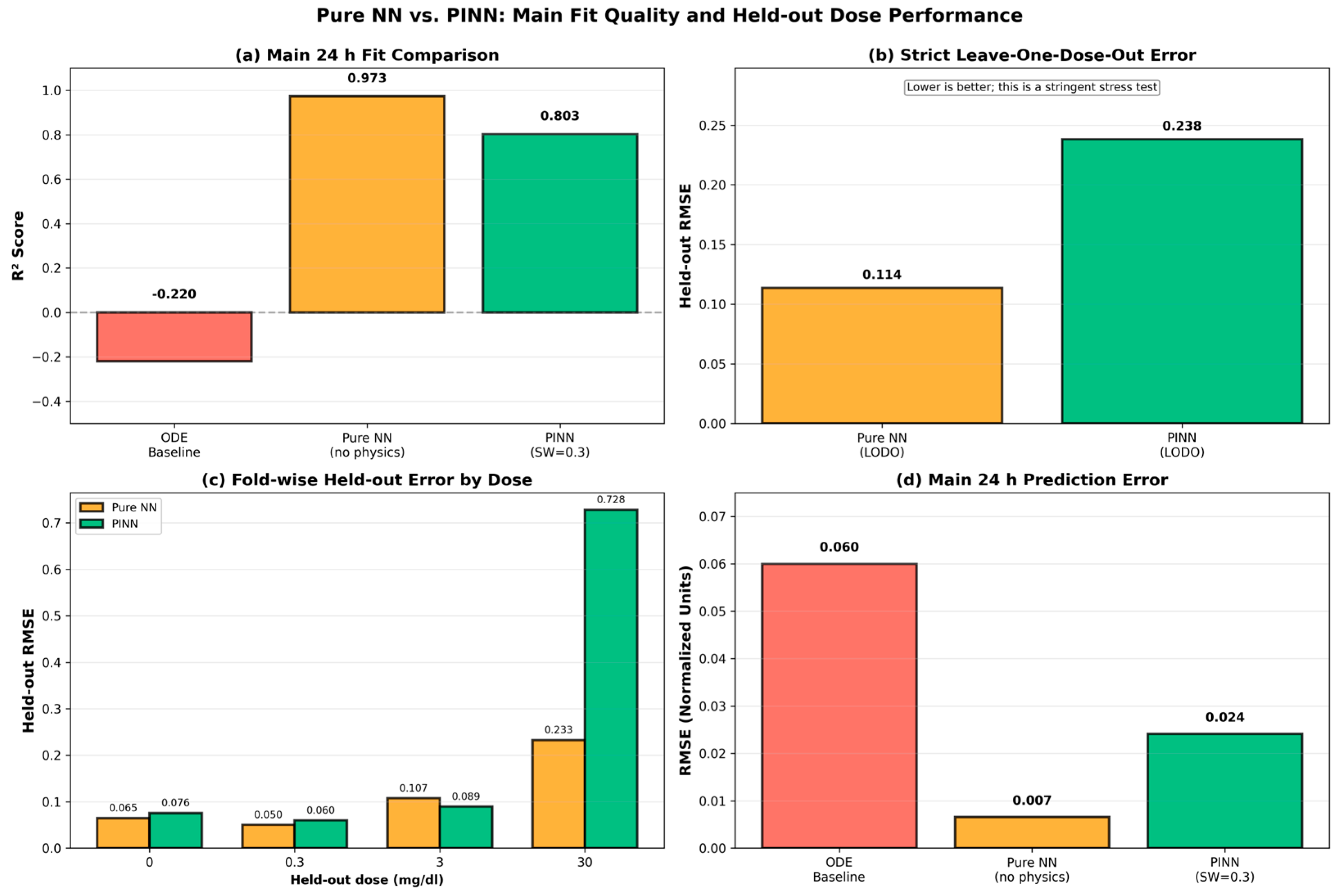
The pure NN ensemble showed clear overfitting behavior. Training performance was very strong, with mean training R² = 0.973 ± 0.040, indicating near-perfect fitting of the observed training data. The corresponding training RMSE was 0.007 ± 0.006, substantially lower than that of the PINN. However, LODO evaluation showed much weaker held-out performance, with mean test RMSE = 0.114. Because each held-out fold contains only one test point, fold-level test R² values are not informative and are therefore not emphasized here.

Table 7. Pure NN vs. PINN performance comparison ¹.

Metric	Pure NN (No Physics)	Accepted PINN Ensemble (SW = 0.3)
Training R2	0.973 ± 0.040	-
Training RMSE	0.007 ± 0.006	-
Held-out RMSE (LODO)	0.114	0.238
Main 24 h ensemble RMSE	-	0.024
Main 24 h ensemble R2	-	0.803

¹ Note: The pure NN values summarize training performance and LODO held-out error. The PINN values distinguish between strict held-out-dose evaluation (LODO RMSE = 0.238) and the main accepted ensemble fit to the full 24 h dataset (RMSE = 0.024, R² = 0.803). Because each held-out fold contains only one test point, fold-level test R² values are not emphasized.

summarizes the contrast between the pure NN baseline and the accepted PINN ensemble.

Fold-level analysis further illustrates the instability of the pure NN baseline under held-out-dose evaluation: Fold 1 (0.0 mg/dL) produced test RMSE = 0.065, Fold 2 (0.3 mg/dL) test RMSE = 0.050, Fold 3 (3.0 mg/dL) test RMSE = 0.107, and Fold 4 (30.0 mg/dL) test RMSE = 0.233. These results indicate that the pure NN can fit the observed training points well, but does not reliably recover dose-level structure from such limited data.

At the same time, the softplus activation successfully enforced non-negativity, showing that simple architectural constraints can prevent obviously unphysical outputs. However, this alone was insufficient to produce stable predictions under sparse observations. Taken together, these results support the role of physics-informed regularization in improving biological consistency relative to an unconstrained neural baseline, while also underscoring that held-out-dose generalization remains difficult for all methods in this severely data-limited setting.

Figure 2 compares Pure NN and PINN performance across four complementary views: main 24 h fit quality, strict LODO error, fold-wise held-out error by dose, and main 24 h prediction error.

Together, these results show that the pure NN fits the observed training data extremely well, whereas the PINN provides the strongest biologically constrained fit to the full dataset, but neither approach generalizes strongly under strict held-out-dose evaluation.

4.6. Pareto Frontier Analysis

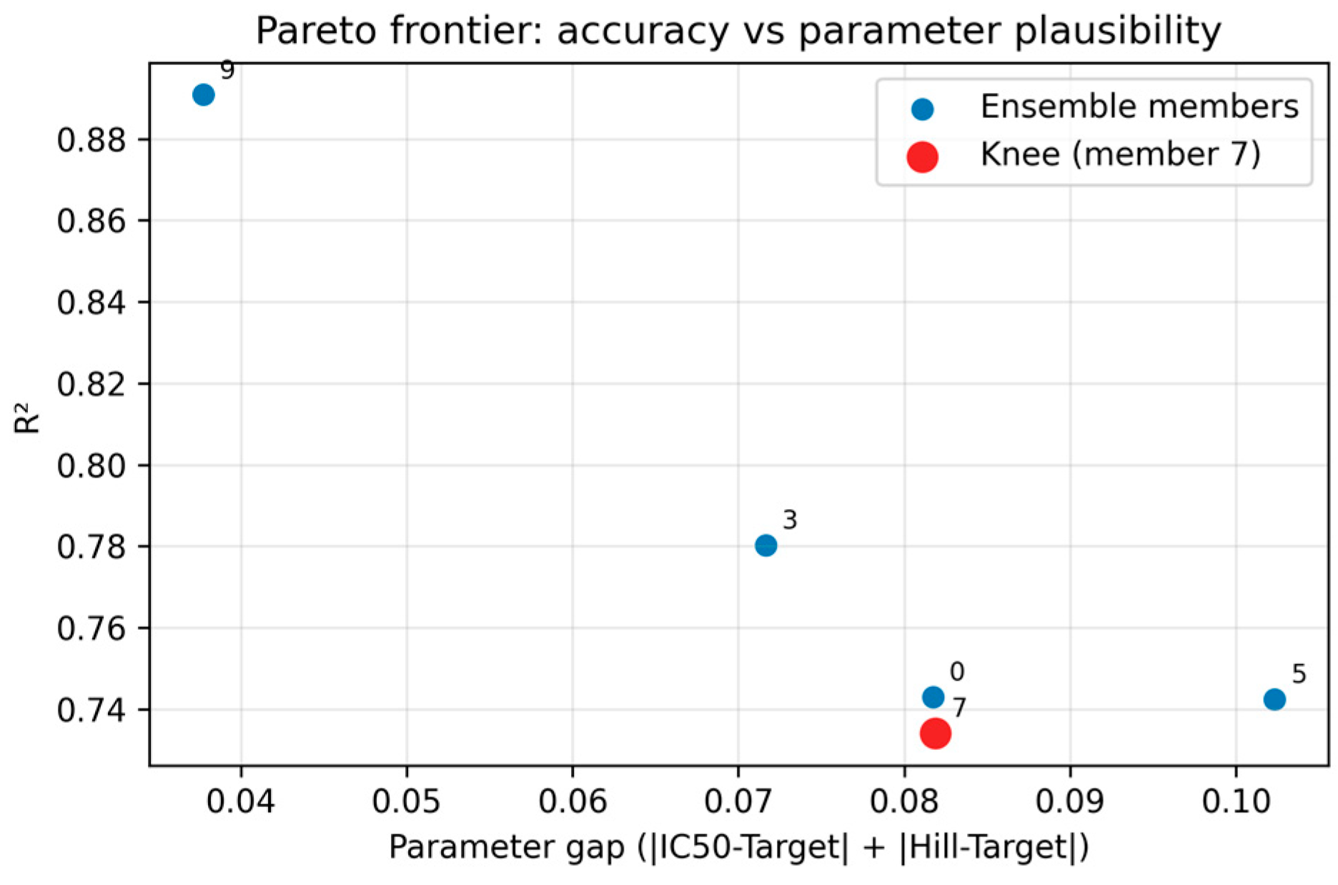
The trade-off between predictive accuracy and parameter plausibility across accepted ensemble members is shown in Figure 3.

The Pareto-style comparison highlights meaningful variation across accepted models. Member 9 represents the strongest single accepted solution, whereas Members 0, 3, 5, and 7 illustrate the initialization sensitivity that remains under severe data sparsity. The spread in member performance (R² ranging from 0.734 to 0.891) supports reporting the accepted ensemble as the primary result rather than relying on a single model. More broadly, this analysis suggests that the SW = 0.3 configuration can produce models that jointly achieve good predictive fit and plausible parameter values, although these solutions should still be interpreted as model-dependent and initialization-sensitive.

4.7. Dose-Response Analysis

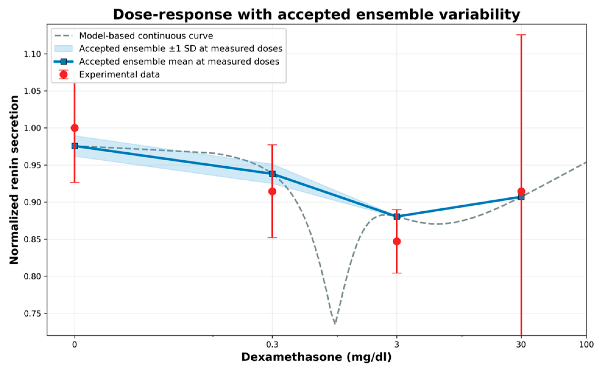
The dose-response relationship predicted by the PINN ensemble is shown in Figure 4.

The model captures the main pattern observed at all four measured doses: (i) control (0 mg/dL), predicted 0.976 ± 0.012 versus observed 1.000; (ii) low dose (0.3 mg/dL), predicted 0.938 ± 0.012 versus observed 0.915; (iii) medium dose (3.0 mg/dL), predicted 0.880 ± 0.001 versus observed 0.847; and (iv) high dose (30.0 mg/dL), predicted 0.907 ± 0.0004 versus observed 0.915. The dose-response profile suggests an overall inhibitory relationship centered near the learned IC₅₀ = 2.925 mg/dL, while also preserving the partial high-dose recovery seen experimentally. Because only four dose conditions were measured, the detailed shape of the interpolated curve between observed points should be interpreted cautiously as a model-dependent trajectory rather than a directly validated biological response.

4.8. Temporal Dynamics Inference

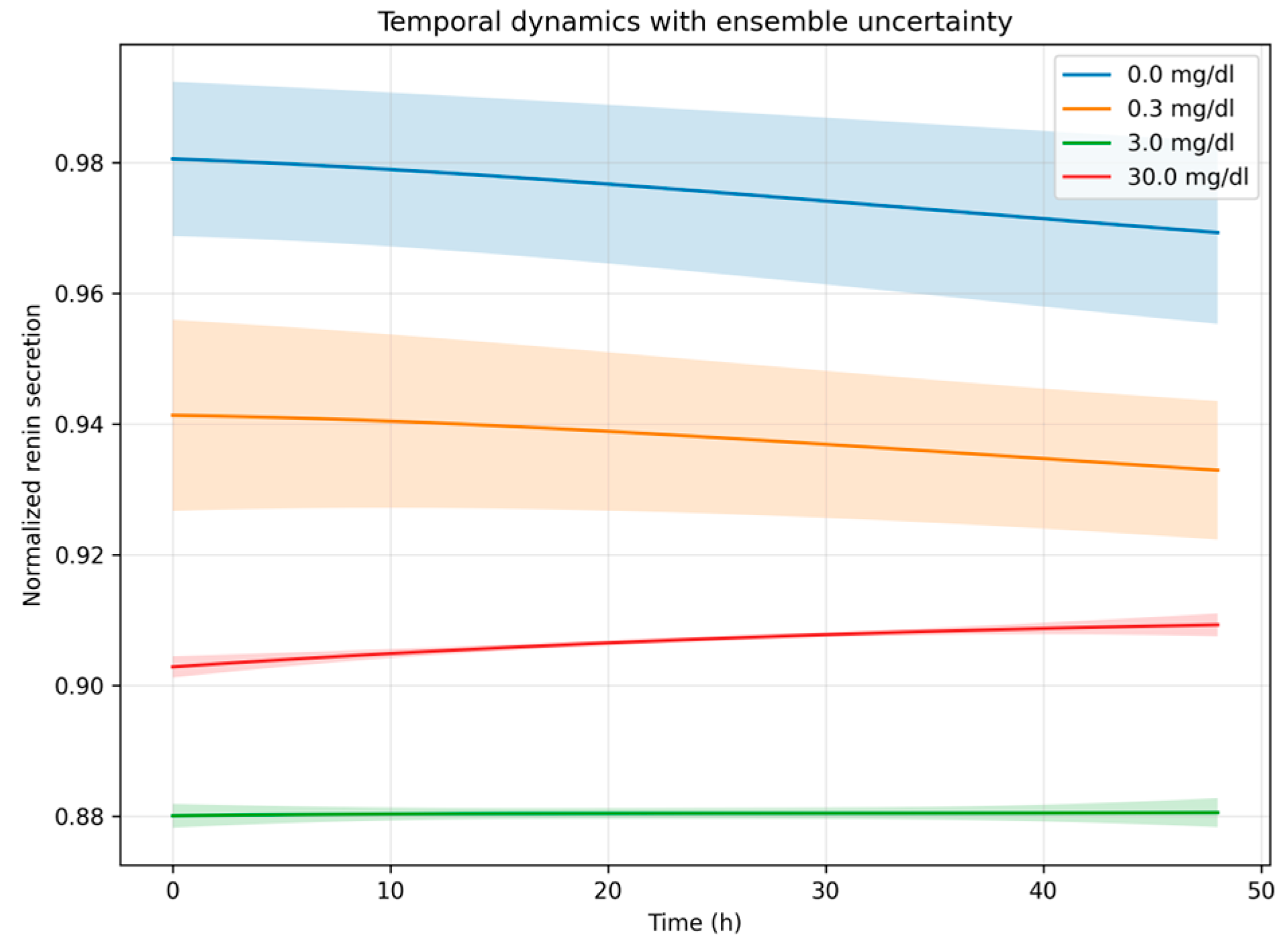
Despite training exclusively on 24-h measurements, the PINN infers complete 48-h time-courses through enforcement of ODE constraints at 512 collocation points. Figure 5 shows the predicted time-courses for secreted renin concentration.

At the control condition (0 mg/dL), secreted renin shows a slight decrease from approximately 0.981 at t = 0 h to 0.969 at t = 48 h. At low dose (0.3 mg/dL), the predicted trajectory decreases modestly from 0.941 to 0.933 over the same interval. At medium dose (3.0 mg/dL), the predicted trajectory remains nearly flat around 0.880, with very small variability across accepted ensemble members. At high dose (30.0 mg/dL), the predicted trajectory shows a slight increase from 0.903 at t = 0 h to 0.909 at t = 48 h, which is qualitatively consistent with the partial high-dose recovery seen in the measured dose-response.

At the training timepoint t = 24 h, the predicted values are 0.975 (control), 0.938 (0.3 mg/dL), 0.880 (3.0 mg/dL), and 0.907 (30.0 mg/dL), matching the ensemble predictions used in the dose-response and performance analyses.

Because no experimental time-series measurements were available, these temporal trajectories should be interpreted as model-dependent, hypothesis-generating solutions consistent with the ODE structure and the 24-h observations, rather than as directly validated biological time-courses.

4.9. Residual Analysis

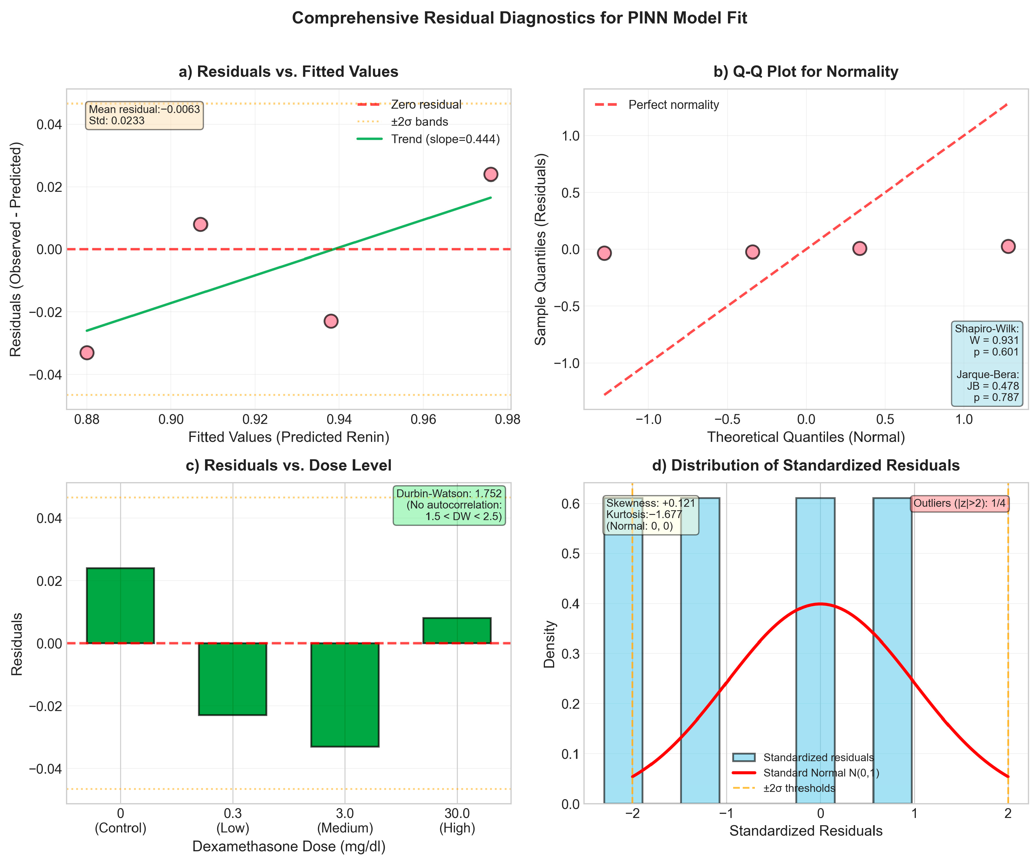
A comprehensive residual analysis was performed to assess model adequacy and to identify possible systematic patterns, as shown in Figure 6.

Residuals (observed minus predicted) were +0.024 (control), −0.024 (0.3 mg/dL), −0.033 (3.0 mg/dL), and +0.008 (30.0 mg/dL). Their absolute magnitudes were small relative to the normalized response scale. Standardized residuals were +1.05, −1.01, −1.44, and +0.32, respectively, with none exceeding ±2. The largest standardized residual occurred at 3.0 mg/dL, where the experimental variance was smallest, and therefore small absolute deviations carry greater relative weight.

Table 8. Residual diagnostic test results.

Test	Statistic	p-Value	Result	Interpretation
Shapiro–Wilk	W = 0.931	0.601	Pass	No strong evidence against normality
Jarque–Bera	JB = 0.478	0.787
Durbin–Watson	DW = 1.752	-		No strong evidence of autocorrelation
Runs Test	z = −1.22	0.221		Residual signs appear broadly random

presents the statistical diagnostic tests.

Shapiro-Wilk (W = 0.931, p = 0.601) and Jarque-Bera (JB = 0.478, p = 0.787) do not reject normality at alpha = 0.05, but these results should be interpreted cautiously because the sample size is only four. The Durbin-Watson statistic, DW = 1.752, does not indicate obvious autocorrelation, and the runs test (z = −1.22, p = 0.221) does not indicate a strong departure from random residual signs. Overall, the residual diagnostics are consistent with an adequate fit to the four observed dose conditions, while remaining too small in sample size to support strong distributional conclusions.

Table 9. Residual distribution statistics.

Statistic	Value
Mean	−0.0063
Std Dev	0.0233
Min	−0.0335
Max	+0.0243
Q1	−0.0260
Median	−0.0080
Q3	+0.0117
Skewness	+0.121
Kurtosis	−1.677

presents summary statistics for the residual distribution.

The mean residual of −0.0063 indicates slight average underestimation, while the residual standard deviation of 0.0233 corresponds to a small spread on the normalized response scale. The skewness and kurtosis values are broadly consistent with an approximately symmetric distribution, but interpretation remains limited by the very small number of observations.

4.10. Cross-Validation and Robustness

A strict LODO analysis was performed as a held-out-dose stress test under extreme data scarcity. In each fold, one of the four dose conditions was withheld, the model was trained on the remaining three conditions, and prediction error was evaluated on the omitted dose. The resulting held-out absolute errors were 0.076 for the control dose (0 mg/dL), 0.060 for 0.3 mg/dL, 0.089 for 3.0 mg/dL, and 0.728 for 30.0 mg/dL.

The average held-out error across folds was 0.238, indicating that cross-dose generalization remains challenging in this setting. In particular, the large error on the 30.0 mg/dL fold shows that the model does not reliably extrapolate high-dose behavior when that condition is absent from training. These results should therefore be interpreted as evidence of limited held-out-dose robustness rather than strong generalization. At the same time, the lower errors for the control, 0.3 mg/dL, and 3.0 mg/dL folds suggest that the framework retains partial interpolation capability among nearby observed dose conditions.

4.11. Validation Against Plausibility Criteria

All five accepted ensemble members (0, 3, 5, 7, and 9) passed the predefined plausibility checks across all four experimental doses. These checks included: (a) non-negativity, with all concentrations remaining ≥ 0 throughout the 48-h simulations; (b) boundedness, with maximum renin secretion ≤ 1.8; (c) smoothness, with maximum temporal derivative ≤ 0.15; (d) approximate steady-state convergence, with the final 12-h window showing std ≤ 0.06; (e) temporal suppression, requiring renin(t = 48 h) ≤ renin(t = 0 h) + 0.03 for treated conditions; and (f) approximate dose monotonicity, requiring renin(dose_{i + 1}) ≤ renin(dose_i) + 0.03 at fixed time. The overall acceptance rate for the SW = 0.3 configuration was 50% (5 of 10 trained models), indicating that these plausibility criteria were selective enough to exclude many candidate solutions while retaining a stable accepted ensemble.

The accepted PINN ensemble, therefore, satisfied both predictive and plausibility-based criteria under the chosen modeling assumptions. At the same time, passing these checks should not be interpreted as proof of biological correctness, but rather as evidence that the accepted solutions remained consistent with the imposed mechanistic and qualitative constraints. Section 5 discusses the biological interpretation of these findings together with the remaining limitations of the approach.

4.12. Supplementary Experiments Results

Supplementary Further methodological checks, including supplementary experiment results for ramped weighting, held-out-dose evaluation, and hyperparameter sensitivity, are reported in the Supplementary Materials.

4.13. Statistical Comparison of Ensemble Configurations

Detailed non-parametric statistical comparison of the SW = 0.3 and SW = 0.5 ensemble configurations is provided in the Supplementary Materials.

4.14. Attempted Global Sensitivity Analysis

The attempted global sensitivity analysis and its limitations under the present sparse-data regime are reported in the Supplementary Materials.

5. Discussion

This section interprets the results within the broader context of glucocorticoid-RAAS biology and computational methodology, addresses limitations revealed through validation, and discusses the broader implications of the framework. Importantly, this study should be interpreted primarily as a proof-of-concept methodological investigation rather than a definitive biological model of glucocorticoid-mediated renin regulation. Because the available data consist of four dose conditions measured at a single 24-h timepoint, neither the biochemical parameters nor the inferred temporal trajectories are uniquely identifiable. Accordingly, the learned parameters and time-courses are best viewed as model-dependent, hypothesis-generating estimates that are consistent with the assumed ODE structure and observed measurements.

5.1. Biological Interpretation of Learned Parameters

The PINN framework recovered parameter values from sparse experimental data that are biologically plausible and useful for generating mechanistic hypotheses about glucocorticoid-renin regulation.

The learned half-maximal inhibitory concentration, IC₅₀ = 2.925 ± 0.012 mg/dL, represents the dexamethasone concentration associated with 50% maximal suppression in the fitted model and lies close to the expected target value used for weak biological regularization. The learned Hill coefficient, h = 1.950 ± 0.009, is also close to the target value and is consistent with a cooperative repression process in the fitted dose-response relationship. In biological terms, h > 1 is compatible with mechanisms such as receptor dimerization, cooperative DNA binding to glucocorticoid response elements, or multi-component transcriptional regulation, all of which are known to occur in glucocorticoid signaling [37,38].

However, these estimates should not be interpreted as uniquely validated biochemical constants, but rather as constrained parameter values supported by the present model and data.

Direct comparison with literature remains difficult because few studies have quantified these specific kinetic parameters in juxtaglomerular cells. Nevertheless, several qualitative points of contact are encouraging. Glucocorticoid receptor nuclear translocation times of 10–20 min have been reported in various cell types using fluorescence microscopy [62,63], which is broadly consistent with the inferred characteristic time of approximately 15 min ($k_{\mathrm{nuclear}}$ = 3.95 h⁻¹). mRNA half-lives for regulatory genes often fall in the range of 0.5 to 2 h in mammalian cells [66], and the inferred renin mRNA half-life of approximately 0.60 h ($k_{\mathrm{deg},\mathrm{renin}}$ = 1.15 h⁻¹) is compatible with a rapidly regulated transcript. Similarly, protein secretion rates in endocrine systems commonly operate on timescales of tens of minutes to about an hour [68], which is broadly consistent with the inferred secretion half-life of 0.46 h ($k_{\mathrm{secretion}}$ = 1.51 h⁻¹).

The inferred kinetic rate constants also reflect the multi-timescale character of the modeled cascade. Renin mRNA turnover occurs on the order of less than an hour, supporting rapid transcriptional responsiveness while maintaining baseline expression through constitutive synthesis ($k_{\mathrm{synth},\mathrm{renin}}$ = 1.31 h⁻¹). Translation proceeds with a characteristic timescale of approximately 26 min ($k_{\mathrm{translation}}$ = 2.28 h⁻¹), while secretion occurs with a half-life of approximately 0.46 h. These values are broadly consistent with a system in which transcription, translation, and secretion remain dynamically coupled over the 24- to 48-h window of the model.

The glucocorticoid receptor-related parameters are also biologically plausible within the model. Nuclear translocation [37] is rapid, with a characteristic time of about 15 min, while receptor turnover occurs with a half-life of approximately 0.62 h ($k_{\mathrm{deg},\mathrm{GR}}$ = 1.12 h⁻¹). The inferred dissociation constant $K_d=k_{\mathrm{unbind}}/k_{\mathrm{bind}}$ = 0.132 mg/dL suggests a relatively high-affinity dexamethasone-receptor interaction in the fitted system, which is qualitatively consistent with the potent activity of synthetic glucocorticoids relative to endogenous cortisol [35,36].

Relative to the ODE-only baseline, the physics-informed framework produced substantially better predictive fit (R² = 0.803 versus −0.220, RMSE = 0.024 versus 0.060) together with tighter agreement across accepted runs. The ODE baseline yielded IC₅₀ = 3.12 ± 0.45 mg/dL and Hill = 2.31 ± 0.28, indicating much larger variability and poorer alignment with expected values. This contrast is consistent with the idea that, under severe data scarcity, unconstrained parameter estimation remains highly unstable.

The improvement obtained by the PINN should be understood as the result of strong regularization rather than proof of full identifiability. In the present framework, ODE residuals at 512 collocation points, initial-condition constraints, and biological plausibility criteria together restrict the space of admissible solutions and favor dynamically consistent trajectories. This helps stabilize parameter estimation in an otherwise ill-posed inverse problem. At the same time, the narrow spread of the accepted ensemble should not be interpreted as evidence that the true biological parameters have been uniquely identified from the available data.

5.2. Calibration of the PINN Objective

One of the main methodological findings of this study is that the intermediate synthetic-data weight SW = 0.3 provided the best overall balance among the tested configurations, yielding the strongest combination of predictive performance, parameter plausibility, and accepted ensemble size.

Systematic exploration across SW ∈ {0.2, 0.3, 0.5} revealed a non-monotonic relationship between synthetic-data weighting and accepted ensemble quality.

Table 10. Success rate and performance across synthetic weight configurations.

Configuration	Trained	Passed	Success Rate	Ensemble Size	R2	Interpretation
SW = 0.2	5	1	20%	n = 1	N/A 1	Exploratory only
SW = 0.3	10	5	50%	n = 5	0.803	Best overall among tested settings
SW = 0.5	10	4	40%	n = 4	0.759	Baseline comparison

¹ Note: Success rate denotes the percentage of trained models passing all plausibility checks. For SW = 0.2, only one model passed, so stable ensemble statistics could not be computed.

summarizes the configuration comparison.

The SW = 0.2 configuration yielded the tightest parameter alignment in the single accepted run, but its low acceptance rate made that result exploratory only. The SW = 0.5 configuration achieved a moderate acceptance rate and good predictive accuracy, but with somewhat weaker parameter alignment. The intermediate SW = 0.3 configuration produced the largest accepted ensemble (n = 5) together with the strongest overall predictive fit (R² = 0.803) and slightly improved parameter alignment relative to SW = 0.5.

These results suggest that synthetic-data weighting should be calibrated rather than assumed to improve performance monotonically. If the synthetic term is too weak, it may provide insufficient guidance; if it is too restrictive, it may reduce the number of solutions that remain both plausible and well-fitted. In the present study, SW = 0.3 provided the most favorable compromise across these competing demands.

The plateau-ramp mechanism for the high-dose constraint also contributed to training stability. By keeping the high-dose penalty weaker during the early phase of training and increasing it gradually, the model was able to learn approximate dose-response behavior before stronger biological constraints were enforced. This is consistent with the supplementary ramp-ablation study, in which ramped weighting improved the plausibility pass rate relative to constant weighting.

A further practical point is that ensemble size matters. The SW = 0.2 configuration illustrates that a single successful run is not sufficient for stable ensemble-level interpretation, even if that individual run appears promising. For this reason, the accepted SW = 0.3 ensemble is emphasized throughout the manuscript: it provided both the strongest overall performance among the tested configurations and a sufficient number of accepted members to support a more stable summary across runs.

Overall, this calibration analysis supports the broader methodological conclusion that, in sparse-data PINN settings, reporting only the best single run is insufficient. Predictive metrics, accepted ensemble size, and plausibility pass rate should all be considered when comparing configurations.

5.3. Non-Monotonic Dose-Response and Possible Saturation Effects

One of the most notable experimental observations is the non-monotonic dose-response curve, with maximal suppression at 3.0 mg/dL and partial recovery at 30.0 mg/dL. The accepted PINN ensemble reproduces this overall pattern, with predicted values of 0.976 for control, 0.938 at 0.3 mg/dL, 0.880 at 3.0 mg/dL, and 0.907 at 30.0 mg/dL. At the same time, both the residual analysis and the large variance observed at the highest dose indicate that the underlying biology is not fully resolved by the current model.

Recent studies point to highly context-dependent glucocorticoid effects on the RAAS: systemic renin suppression in Cushing’s syndrome with simultaneous adipose renin upregulation [4]; developmental RAAS programming after prenatal dexamethasone exposure [5]; dexamethasone-mediated suppression of ACE2 in pancreatic tissue [6], and reduced Ang II levels in inflammatory settings such as sepsis [39]. These findings support the possibility that the partial recovery at high dose reflects multiple interacting mechanisms rather than a single monotonic repression process.

Several non-exclusive biological explanations are consistent with the observed pattern. One possibility is receptor saturation, whereby increasing ligand concentration beyond a certain level no longer yields proportional additional repression because receptor occupancy, nuclear binding capacity, or co-regulator availability becomes limiting. A second possibility is engagement of additional pathways at very high concentrations, including off-target receptor effects or stress-response pathways that partially counteract renin suppression. A third possibility is adaptive regulation of glucocorticoid receptor responsiveness during high-dose exposure, for example, through altered receptor abundance or receptor-state regulation. The present data do not allow these mechanisms to be distinguished directly, but the observed partial recovery at 30.0 mg/dL is qualitatively consistent with such possibilities.

The experimental variance structure is also informative. The standard deviation at 30.0 mg/dL (5.93 ng/mL) is approximately fivefold larger than at 3.0 mg/dL (1.17 ng/mL), indicating much greater heterogeneity at the highest dose. This may be consistent with heterogeneous saturation or heterogeneous cellular responsiveness, although alternative explanations are also possible. Because the measurements are bulk ELISA readouts rather than single-cell trajectories, the variance increase should be interpreted cautiously.

The current model captures the overall non-monotonic pattern but does so through a relatively simple phenomenological suppression structure. In principle, the model could be extended to include explicit residual suppression terms, receptor-pool limitations, or adaptive receptor-regulation dynamics. Such extensions might provide a more explicit mechanistic representation of high-dose behavior. However, adding further parameters to a model trained on only four dose conditions would substantially worsen identifiability and increase overfitting risk.

For this reason, the current study does not attempt to discriminate formally among alternative saturation or compensation mechanisms. Instead, the non-monotonic response is best interpreted as an experimentally constrained feature that the physics-informed model is able to reproduce, while the precise biological explanation remains open. Future work with richer dose sampling, multi-timepoint measurements, and perturbation experiments will be needed to test whether receptor saturation, compensatory signaling, or other mechanisms are responsible for the partial high-dose recovery.

5.4. Temporal Dynamics Inference from Single Timepoints

A notable capability of the PINN framework is that it produces complete 48-h trajectories despite being trained only on measurements at 24 h. This temporal inference arises because the neural-network surrogate is constrained not only by the observed data but also by the ODE residuals evaluated across the full simulation window and by the initial-condition constraints.

The key idea is that differential equations impose structural links between behavior at different times. For a dynamical system $dy/dt=f(y,t,\theta )$, agreement with the governing equations at dense collocation points constrains the set of admissible trajectories even when direct measurements are sparse. In the present framework, the data term constrains predictions at $t$ = 24 h, while the physics loss and initial-condition loss require consistency across the full temporal domain. This is what allows the model to generate temporally continuous trajectories from single-timepoint observations.

At the same time, these inferred time-courses cannot be treated as directly validated biological dynamics. Without experimental time-series measurements, the temporal profiles remain model-dependent extrapolations. Several features of the inferred trajectories are nevertheless qualitatively plausible: they are smooth, internally consistent across doses, and compatible with the timescales implied by the fitted kinetic parameters. The predicted trajectories also remain numerically stable over longer simulation windows, which supports the internal consistency of the learned solution.

Even so, the inferred temporal dynamics should be interpreted as one plausible family of trajectories rather than as the uniquely correct biological time-course. Alternative parameter sets or alternative mechanistic formulations could produce different temporal behavior while remaining consistent with the same 24-h measurements. This limitation is intrinsic to the sparse-data setting and cannot be removed by the PINN alone.

The temporal predictions are therefore most useful as experimentally testable hypotheses. For example, the model suggests early renin mRNA dynamics on the scale of hours, relatively stable secreted-renin trajectories between 12 and 48 h, and rapid glucocorticoid receptor-related dynamics at early times. These predictions can guide future experiments, including multi-timepoint qRT-PCR, intracellular protein measurements, and subcellular receptor localization assays. Such experiments would provide the direct time-series information needed to confirm, refine, or reject the model-inferred trajectories.

5.5. Uncertainty Quantification and Ensemble Aggregation

The final framework summarizes uncertainty primarily through deterministic ensemble aggregation across multiple accepted models with different initializations. Monte Carlo dropout was explored separately as an auxiliary analysis, but it is not the primary uncertainty result used in the final interpretation of this study.

The narrow spread of some parameter estimates (IC₅₀: σ = 0.012, Hill: σ = 0.009) most likely reflects strong regularization from the physics-informed objective and the restricted set of accepted solutions, rather than genuine certainty about the underlying biological parameters. In other words, agreement across accepted models should not be confused with full identifiability.

Ensemble aggregation across n = 5 accepted models provides three practical benefits. First, the ensemble mean provides a more stable summary than any single model, reducing sensitivity to initialization-specific behavior. Second, ensemble standard deviation provides a descriptive measure of model-to-model variability across accepted runs. Third, comparison across individual accepted members helps reveal the extent to which the results depend on optimization path or initialization, as illustrated by the spread from R² = 0.734 to R² = 0.891 across accepted models.

At the same time, the uncertainty captured here is only partial. Ensemble spread reflects sensitivity to initialization and optimization under the assumed model structure, but it does not account for all important sources of uncertainty. In particular, it does not fully capture measurement-noise uncertainty, structural uncertainty arising from simplifications in the ODE model, or uncertainty associated with alternative mechanistic formulations. For this reason, the current uncertainty summary should be interpreted as a practical descriptive measure rather than a full probabilistic uncertainty decomposition.

The tighter ensemble agreement observed near some dose conditions, such as 3.0 mg/dL, likely reflects stronger constraint from the available data and the fitted dynamics in those regions, whereas wider spread at other conditions reflects greater ambiguity. However, even these patterns should be interpreted cautiously, since model misspecification and sparse observations may produce overconfident uncertainty estimates. A more complete uncertainty treatment would require hierarchical or Bayesian formulations that explicitly account for measurement noise and structural model uncertainty.

5.6. Clinical Implications and Translational Potential

The ability to model glucocorticoid effects on renin expression may eventually have translational relevance for hypertension risk during glucocorticoid therapy, although the present study remains far from direct clinical application.

Approximately 30% of patients receiving chronic glucocorticoid therapy develop hypertension [1,2], yet predicting individual susceptibility remains difficult. Recent clinical studies in Cushing’s syndrome support the idea that systemic and tissue-specific RAAS regulation may diverge during glucocorticoid excess [4]. Together with developmental studies showing long-term RAAS consequences of prenatal dexamethasone exposure [5], these findings suggest that glucocorticoid effects on renin and related pathways may be clinically important, but also highly context-dependent.

The learned IC₅₀ = 2.925 mg/dL places the fitted dose-response in a concentration range where changes in dexamethasone exposure could meaningfully alter modeled renin suppression. In principle, this suggests a possible future role for integrating mechanistic response models with pharmacokinetic information to estimate individual glucocorticoid exposure-response relationships. Such an approach could eventually support more personalized monitoring strategies, especially in patients at elevated cardiovascular risk.

At the same time, any translational interpretation must remain highly cautious. The present model is based on an in vitro mouse juxtaglomerular-like cell line, a simplified ODE structure, and measurements taken at only one experimental timepoint. It does not capture the full physiological complexity of blood-pressure regulation, including systemic feedback loops, tissue-specific RAAS signaling, sympathetic control, vascular effects, or the contributions of non-renal renin sources. It also focuses specifically on dexamethasone and therefore cannot be assumed to generalize directly to other glucocorticoids with different receptor-binding and pharmacokinetic profiles.

For these reasons, the current work should not be interpreted as a basis for clinical dosing decisions or intervention strategies. Rather, its translational value lies in showing that physics-informed modeling may help organize sparse mechanistic data and generate testable hypotheses about glucocorticoid-RAAS interactions. A realistic translational pathway would require additional validation in human-relevant cellular systems, richer time-resolved datasets, integration with pharmacokinetics, and ultimately, prospective clinical studies.

5.7. Broader Methodological Relevance

Beyond the specific glucocorticoid-renin application, this study illustrates several methodological lessons for modeling under severe data scarcity in biology. Many biomedical problems share the same general structure: partial mechanistic knowledge, limited and expensive measurements, and a parameter space that is too large for stable estimation using standard approaches alone.

In such settings, purely data-driven models can fit sparse observations but may generalize poorly and need not respect biological constraints, whereas classical mechanistic parameter estimation can remain highly unstable because many parameter combinations produce similarly acceptable fits. Physics-informed learning offers a useful intermediate strategy by embedding mechanistic structure directly into the training objective.

Several practical lessons from the present study may generalize to other sparse-data applications. First, calibration of the loss terms matters: the relative weighting of observational, mechanistic, and biological constraints can materially affect both fit quality and model acceptance. Second, adaptive training schedules can improve stability when different constraints become important at different stages of optimization. Third, ensemble-based reporting is preferable to single-model reporting in underdetermined settings because it exposes initialization sensitivity and provides a more stable summary across accepted runs. Fourth, explicit plausibility criteria help make the modeling assumptions transparent, even though they do not resolve the deeper identifiability problem.

These ideas may be relevant to other hormone-regulated or signaling-driven systems in which mechanistic structure is known but dense longitudinal data are unavailable. Potential examples include aldosterone signaling, thyroid hormone regulation, insulin-response pathways, and other endocrine or signaling networks that operate across multiple timescales. In such settings, the precise model structure would differ, but the general workflow of combining sparse measurements with ODE-based constraints could still be useful.

At the same time, the broader methodological promise of PINNs in biology should not be overstated. Several important limitations remain. The results depend on the assumed ODE structure, so model misspecification remains a major concern. Computational cost can also be substantial when multiple configurations and ensembles must be trained. More fundamentally, physics-informed regularization can improve stability without guaranteeing true parameter identifiability. Finally, biological constraint design still requires substantial domain knowledge and is not yet automatic.

For these reasons, the present work is best viewed as a proof-of-concept example of how physics-informed modeling can be used to organize sparse biological data into mechanistically constrained hypotheses. Its broader contribution is methodological: it shows a workable approach for combining mechanistic priors, sparse measurements, and ensemble-based evaluation in situations where neither purely data-driven nor purely mechanistic fitting is satisfactory on its own.

5.8. Limitations and Future Improvements

Several important limitations should be emphasized. First, the training data are extremely sparse: only four dose conditions were measured, all at a single 24-h timepoint. This severely limits identifiability and prevents direct validation of the inferred temporal dynamics. Additional dose levels, especially between 0.3 and 3.0 mg/dL, together with multi-timepoint measurements, would be the most important improvement for future work.

Second, the mechanistic model is intentionally simplified. The six-state ODE system does not include several potentially relevant regulatory processes, such as post-transcriptional regulation, chromatin-state effects, or broader RAAS feedback mechanisms. Although adding these mechanisms might improve biological realism, doing so with the current dataset would likely worsen overfitting and identifiability problems.

Third, the study is based on a single mouse juxtaglomerular-like cell line, As4.1 (8), (40). Species differences, cell-line adaptation, and the transformed nature of the model system may all limit generalizability to primary human cells or in vivo physiology. Future validation in additional experimental systems, especially human-relevant systems, will therefore be necessary.

Fourth, uncertainty quantification remains incomplete. The current results summarize variability across accepted ensemble members, but they do not provide a full uncertainty decomposition that includes measurement noise, structural model uncertainty, and alternative mechanistic formulations. Likewise, the attempted Sobol analysis was unstable, reinforcing that parameter sensitivity and identifiability remain difficult to characterize in this sparse-data regime.

Fifth, the strict LODO analysis showed limited held-out-dose robustness, particularly when the 30.0 mg/dL condition was omitted. This indicates that the current framework should not be interpreted as strongly generalizing across dose conditions, especially in extrapolative settings.

Several future directions are particularly promising. The most important is richer experimental design: multi-dose, multi-timepoint measurements would immediately improve identifiability and allow direct testing of the model-inferred dynamics. Multi-assay integration, for example, combining ELISA with mRNA, intracellular protein, or receptor-localization measurements, could further constrain the latent states. Single-cell measurements could help clarify whether the high-dose variance reflects heterogeneous cellular responses. Mechanistic perturbation experiments could also help discriminate between possible explanations for the non-monotonic high-dose behavior. Finally, extension to human-relevant systems and eventual coupling to pharmacokinetic models would be natural next steps if richer validation data become available.

Overall, the present study should be viewed as a constrained proof-of-concept under severe data scarcity. Its main value lies in showing that a physics-informed framework can organize sparse measurements into mechanistically structured, testable hypotheses, while also making clear where the current data are insufficient for stronger biological claims.

6. Conclusions

This work presents, to our knowledge, the first application of a physics-informed neural network to model glucocorticoid-mediated renin regulation from severely sparse experimental data. By combining a mechanistic ODE system with a neural-network surrogate, the framework enabled joint estimation of latent dynamics and biochemical parameters from only 36 observations collected at a single 24-h timepoint.

Among the tested configurations, the intermediate synthetic-data weight SW = 0.3 provided the best overall balance between predictive fit, parameter plausibility, and accepted ensemble size. The accepted ensemble achieved R² = 0.803 and RMSE = 0.024, compared with R² = 0.759 for the SW = 0.5 PINN baseline and R² = −0.220 for the ODE-only baseline. Information criteria also favored the PINN over the ODE baseline, with approximately 77× improvement in AIC and 5.9× improvement in BIC. The accepted ensemble yielded IC₅₀ = 2.925 ± 0.012 mg/dL and Hill coefficient = 1.950 ± 0.009, values that are biologically plausible within the assumptions of the model.

The framework also reproduced the experimentally observed non-monotonic dose-response pattern, including partial recovery at the highest tested dose, and generated complete 48-h trajectories despite being trained only at 24 h. However, these inferred temporal dynamics should be interpreted as model-dependent, hypothesis-generating trajectories rather than directly validated biological time-courses. Likewise, the narrow spread of some parameter estimates reflects strong regularization and agreement across accepted models, not definitive proof of full identifiability.

Several limitations remain important. The data are restricted to four dose conditions at one timepoint, the mechanistic model is simplified, the biological system is a mouse cell line rather than a human system, and the strict held-out-dose analysis showed limited cross-dose robustness, especially at the highest dose. The attempted global sensitivity analysis was also unstable, further underscoring the weak identifiability of the present setting.

Overall, the study should be viewed as a proof-of-concept methodological contribution rather than a definitive biological model of glucocorticoid-renin regulation. Its main contribution is to show that physics-informed learning can provide a structured and transparent way to combine sparse measurements with mechanistic constraints when traditional fitting approaches are unstable and purely data-driven models are poorly constrained. Future work should prioritize richer multi-timepoint experiments, human-relevant validation systems, stronger uncertainty quantification, and experimental testing of the model-generated hypotheses. The full Python implementation, together with supporting figures, tables, and data, is available in the GitHub repository cited in [72].