Atmospheric Exposures and Cardiovascular Mortality in United States Counties: Formaldehyde and Wet-Bulb Temperature as Leading Predictors

Abstract

Cardiovascular disease (CVD) is the leading cause of mortality in the United States, yet the role of atmospheric exposures as independent predictors of county-level CVD mortality remains poorly characterized. We integrated satellite-derived atmospheric data alongside socioeconomic, demographic, and livestock predictors across 24,487 county-year observations in the contiguous United States (2012–2019) and applied an XGBoost model with SHAP-based interpretability to identify the leading predictors of county-level CVD mortality (Test R² = 0.706, RMSE = 29.55 per 100,000 persons). Four of the top ten predictors came from CAMS/ERA5. Ambient formaldehyde exposure frequency ranked second among all 43 predictors, exceeded only by educational attainment and surpassing poverty rate. Wet-bulb temperature ranked third, Leaf Area Index for High Vegetation ranked seventh, and sulphate aerosol mixing ratio ranked eighth. These variables added county-level prediction information beyond socioeconomic covariates. Integrating atmospheric exposure monitoring into county-level CVD surveillance alongside socioeconomic indicators may improve the identification of high-risk geographies.

1. Introduction

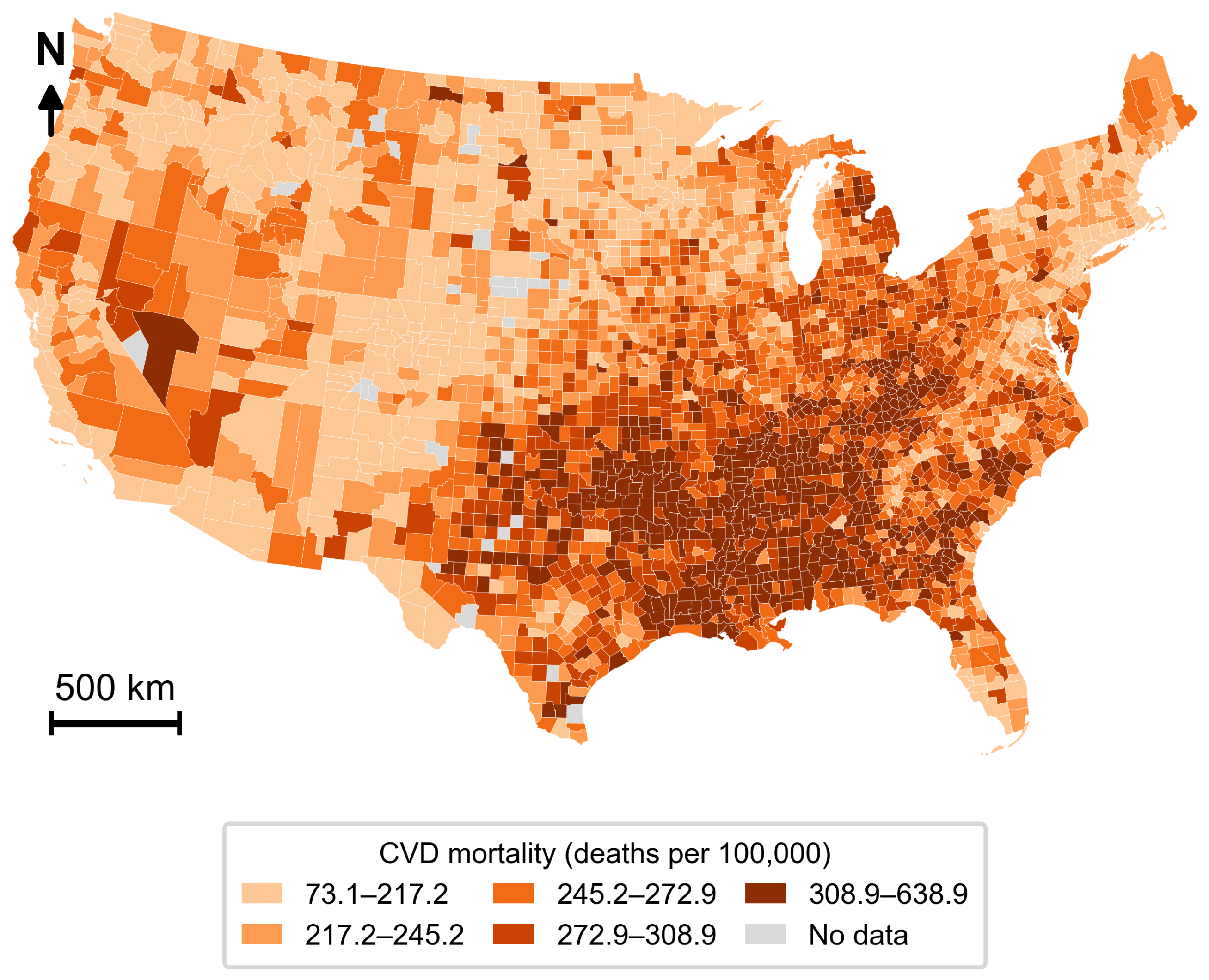
Cardiovascular disease (CVD) is the leading cause of mortality in the United States, responsible for 941,652 deaths in 2022, surpassing all forms of cancer and unintentional injuries combined [1]. Despite substantial declines in age-standardized CVD mortality rates over the past four decades, progress has been unevenly distributed across the country. County-level analyses reveal persistent geographic disparities in CVD burden, with the highest mortality concentration extending from southeastern Oklahoma along the Mississippi River Valley to eastern Kentucky [2]. As shown in Figure 1, county-level CVD mortality rates in 2019 ranged from approximately 73 to 639 deaths per 100,000 persons. These patterns suggest that CVD mortality reflects not only individual clinical risk factors but also place-based socioeconomic and environmental conditions that remain incompletely characterized.

The socioeconomic determinants of CVD mortality are well established. Lower socioeconomic position is associated with greater prevalence of cardiovascular risk factors and higher CVD incidence and mortality [3], with low socioeconomic status conferring cardiovascular risk comparable to traditional clinical risk factors [4]. Socioeconomic disadvantage is also associated with higher rates of smoking, physical inactivity, and poor diet, each of which amplifies cardiovascular risk [5]. Higher educational attainment, in turn, is linked to better employment prospects, greater health literacy, and improved access to preventive care [6]. Despite the predictive strength of these socioeconomic factors, they do not fully account for the geographic variation in CVD mortality observed across US counties, pointing to a role for environmental exposures that operate independently of socioeconomic conditions.

Atmospheric exposures have emerged as an independent class of cardiovascular disease determinants. Air pollutants, including fine particulate matter (PM_2.5) and nitrogen dioxide, promote oxidative stress, immune cell activation, and vascular endothelial dysfunction, all established pathways to cardiovascular disease [7]. PM_2.5 is a mixture of particles and chemical constituents, including heavy metals, that can intensify oxidative stress and vascular injury [8,9]. Long-term PM_2.5 exposure has been associated with an 8.8% increase in cardiovascular disease mortality per 10 μg/m³ increase in concentration, based on a study of 53 million US Medicare beneficiaries, with no evidence of a lower safe threshold [10]. A 2026 umbrella review reported associations between PM_2.5 exposure and cardiovascular outcomes, including myocardial infarction, stroke, heart failure, arrhythmia, and cardiovascular mortality [11]. Formaldehyde, a ubiquitous indoor and ambient air pollutant, has received comparatively little attention in cardiovascular research. Like PM_2.5, it promotes oxidative stress through reactive oxygen species generation and glutathione depletion [12]. Experimental and epidemiological evidence further shows that formaldehyde exposure induces arrhythmia, myocardial infarction, heart failure, and atherosclerosis [13], and that ambient concentrations are associated with short-term increases in circulatory disease mortality [14]. Extreme heat and humidity, measured by wet-bulb temperature, also contribute to cardiovascular morbidity and excess mortality during heat events [7,15]. Similar exposure–mortality relationships have been studied outside the United States, including long-term air pollution exposure in Canada and temperature-related mortality across multiple countries [16,17]. Ground-based monitoring of ambient formaldehyde is spatially sparse across the United States [18,19]. Satellite-derived atmospheric reanalysis products fill this gap, enabling county-level exposure characterization at national scale.

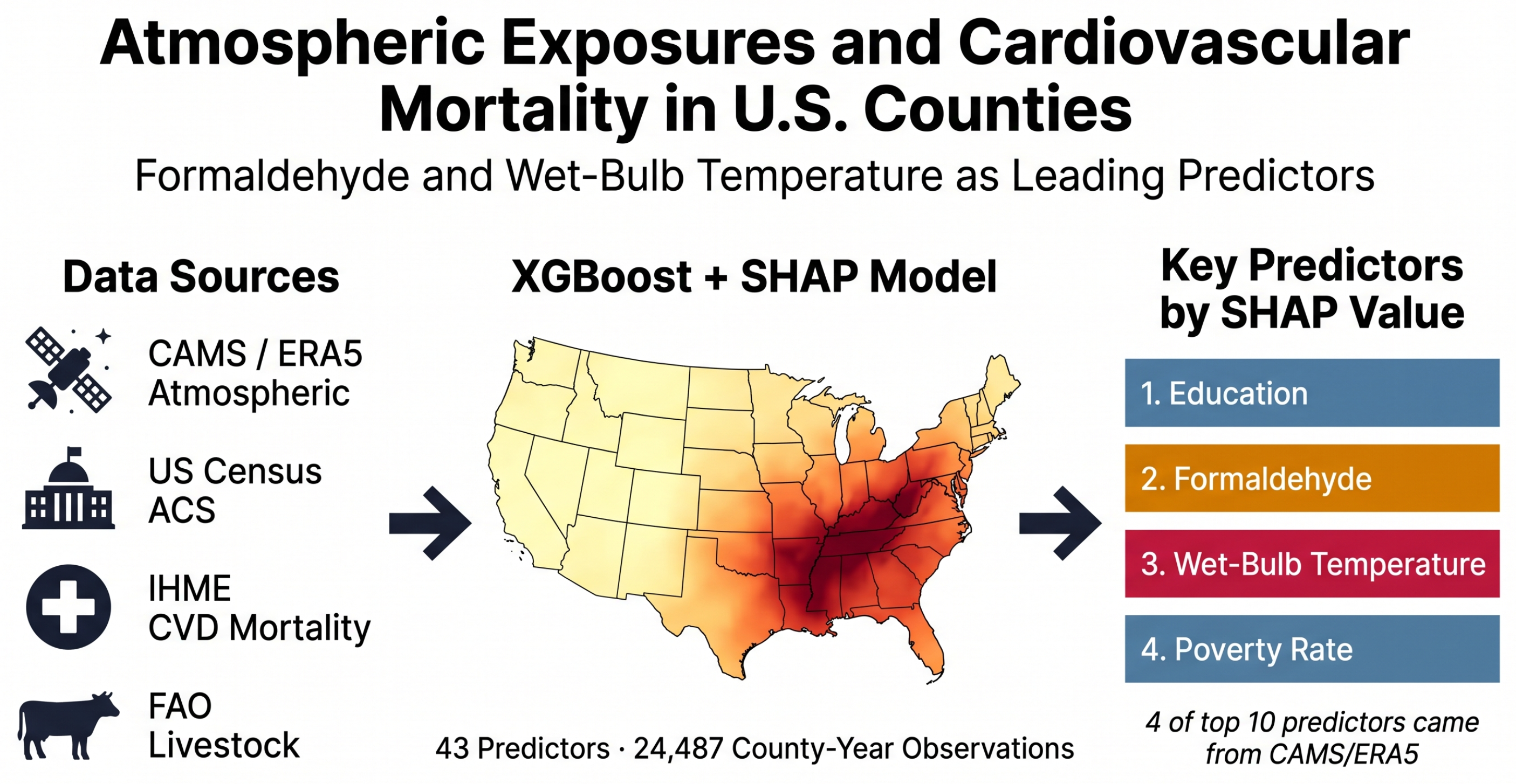
Despite growing evidence for both socioeconomic and atmospheric contributors to CVD mortality, to our knowledge, no prior study has integrated these exposure classes within a unified predictive framework at the US county level. We address this gap using an XGBoost model [20] with SHAP-based interpretability [21] and Bayesian hyperparameter optimization [22], applied to 24,487 county-year observations from 2012 to 2019. Our dataset integrates CVD mortality from the Institute for Health Metrics and Evaluation [23], socioeconomic data from the US Census American Community Survey [24], satellite-derived atmospheric and meteorological data from the Copernicus Atmosphere Monitoring Service and ERA5 reanalysis [25], and livestock density from the Food and Agriculture Organization Gridded Livestock of the World [26]. Among 43 predictors, educational attainment, ambient formaldehyde, and wet-bulb temperature were the three highest-ranked predictors of county-level CVD mortality, with implications for environmental surveillance and cardiovascular public health. The study workflow is shown in Figure 2. Code and processed data are publicly available at https://github.com/mi3nts/predicting-cvd (accessed on 15 June 2026).

2. Methodology

This study constructs a county-year panel dataset covering 3061 counties in the contiguous United States from 2012 to 2019. Four data sources were integrated to build the predictor and outcome variables: IHME cause-of-death estimates provided the target variable, the American Community Survey (ACS) contributed socioeconomic and demographic predictors, the Copernicus Atmosphere Monitoring Service (CAMS) and ERA5 reanalysis supplied atmospheric and meteorological predictors, and the Food and Agriculture Organization Gridded Livestock of the World (FAO GLW) provided livestock density features. An XGBoost regression model was trained with hyperparameters selected via Bayesian optimization. Model performance is reported as root mean square error (RMSE, in deaths per 100,000 persons) and the coefficient of determination (R²). Predictor contributions are quantified and ranked using SHAP values.

2.1. IHME Dataset

The target variable is the age-standardized cardiovascular disease (CVD) mortality rate, expressed as deaths per 100,000 persons. Counties with older populations naturally have higher CVD mortality. Age standardization adjusts for this, producing rates that are directly comparable across counties regardless of their age structure. Estimates were drawn from the IHME Cause of Death dataset (released June 2023), which integrates county-level vital registration records and population data to produce annual, cause-specific mortality estimates for the contiguous United States [23]. The dataset was accessed through the Global Health Data Exchange (GHDx), the public IHME data repository. The records were filtered to retain estimates for the total population across all racial groups and age-standardized mortality rates at the county level. The raw mortality proportion was converted to deaths per 100,000 persons for numerical stability and to conform with standard epidemiological reporting conventions. Data from 2012 to 2019 were selected to align temporally with the available predictor data from the ACS and CAMS sources.

2.2. American Community Survey Dataset

Socioeconomic and demographic predictors were obtained from the American Community Survey (ACS) five-year estimates, published by the US Census Bureau [24]. Five-year pooled estimates were used rather than one-year estimates because many counties, particularly rural ones, have populations too small for stable annual estimates, and for some smaller counties, one-year ACS data are not published at all. Pooling five years of survey data reduces margins of error and ensures full county coverage. The variables were retrieved from the Census Bureau ACS five-year API at the county level and covered poverty, income, educational attainment, unemployment, racial and ethnic composition, disability, and household characteristics. The complete list is provided in Appendix A. A total of 19 variables were initially retrieved. Ten were retained as predictors following the feature reduction procedure described in Section 2.5. Together, they cover the key socioeconomic determinants of CVD risk: income, education, poverty, and demographic composition.

2.3. CAMS and ERA5 Atmospheric Dataset

Atmospheric and meteorological predictor variables were derived from the CAMS EAC4 global reanalysis and the ERA5 reanalysis, both produced by the European Centre for Medium-Range Weather Forecasts (ECMWF) [25]. These products were used because many of the atmospheric and meteorological variables in this study are not measured by ground monitors in every county. Gridded reanalysis fills this gap by providing national coverage for every study year. CAMS EAC4 integrates satellite retrievals from the Ozone Monitoring Instrument (OMI), the Moderate Resolution Imaging Spectroradiometer (MODIS), and the Global Ozone Monitoring Experiment-2 (GOME-2) with atmospheric model assimilation to produce retrospective estimates of atmospheric composition at 0.75° × 0.75° horizontal resolution. ERA5 contributes relative humidity at 0.25° resolution, as this variable is not available in CAMS EAC4. The CAMS and ERA5 files were obtained from the Copernicus/ECMWF data services. Three-hourly model output was averaged to produce annual mean concentrations for each variable. Fraction-of-Time (FoT) metrics were also computed for selected variables, defined as the proportion of three-hourly readings in a given year that exceeded the 75th percentile of that variable’s long-term distribution. The 75th percentile marks values that are higher than typical for the full dataset. Counting how often a county is above this level captures repeated high-exposure periods during the year, not rare extreme events. Because FoT is computed at the county level, it should not be read as an individual person’s short-term exposure. Annual values at county locations were obtained by multilinear interpolation of grid-point output to county boundary sample points, then averaged across sample points to produce a single county-level annual estimate. A total of 46 candidate atmospheric variables were analyzed. Of these, 26 were retained following the feature reduction procedure described in Section 2.5.

2.4. Livestock Dataset

Livestock density data were obtained from the Food and Agriculture Organization Gridded Livestock of the World (FAO GLW) dataset [26], which provides gridded population estimates for seven species at approximately 10 km spatial resolution: cattle, pigs, chickens, horses, sheep, goats, and ducks. GLW is a modeled geospatial product, not a direct sensor measurement of animal locations. It disaggregates livestock census and statistical records to a regular grid using spatial covariates such as land cover and environmental suitability. County-level densities were computed using area-weighted zonal statistics applied to a 2019 National Land Cover Database (NLCD) land-use mask. GLW estimates are available at approximately five-year intervals (2010, 2015, and 2020). Values for the intervening years from 2012 to 2019 were obtained by linear interpolation. Livestock operations are a recognized source of ammonia (NH₃), methane (CH₄), and nitrous oxide (N₂O) emissions, which contribute to regional atmospheric degradation and may elevate ambient concentrations of secondary pollutants associated with cardiovascular disease burden [27]. Seven livestock density features were retained in the final dataset. The four data sources and retained feature counts are summarized in

Table 1. Summary of data sources used to construct the county-year panel dataset (2012–2019).

Source	Description	Features (N)
IHME	Age-standardized CVD mortality rate (deaths per 100,000)	1 (target)
ACS 5-year estimates	Socioeconomic and demographic predictors	10
CAMS/ERA5	Atmospheric and meteorological predictors	26
FAO GLW	Livestock density by species	7
Total predictors		43

.

2.5. Data Processing

The final integrated dataset includes 24,487 county-year observations across 3061 US counties from 2012 to 2019, assembled by merging the four source datasets on county FIPS code and year. Records with missing values were excluded via listwise deletion. Multicollinearity was reduced by identifying predictor pairs with $\left|r\right|>0.85$ and keeping one representative feature from each highly correlated pair. The retained feature was chosen based on stronger correlation with CVD mortality, lower variance inflation factor, and clearer physical or demographic interpretation. For atmospheric variables, this meant favoring measures that were easier to interpret as county-level environmental conditions when two products carried similar information. This reduced the initial candidate predictor pool to the 43 features retained in the final model. The dataset was partitioned into training and test sets using GroupShuffleSplit with a test fraction of 0.20 and county FIPS code as the grouping variable, so that no county appears in both partitions. This ensures the model is evaluated on counties not seen during training. The resulting partition yields 19,583 training observations across 2448 counties and 4904 test observations across 613 counties, with no county overlap between sets.

2.6. Modeling Approach

The modeling objective was to predict county-level age-standardized CVD mortality rates from the 43-feature predictor set. An XGBoost regression model [20] was trained as the primary estimator. Hyperparameters were selected using BayesSearchCV from the scikit-optimize library [22], which uses a Gaussian process surrogate model to explore the hyperparameter space more efficiently than grid or random search. The search ran for 30 iterations with 5-fold GroupKFold cross-validation, using county FIPS as the grouping variable to prevent data leakage across folds. Model selection was based on R² scoring.

Table 2. XGBoost hyperparameter search bounds and optimal values selected by BayesSearchCV.

Parameter	Search Range	Optimal Value
n_estimators	150–800	800
max_depth	3–7	5
learning_rate	0.03–0.25 (log-uniform)	0.03
subsample	0.60–0.90	0.7042
colsample_bytree	0.50–0.85	0.7814
reg_alpha	0.05–8.0 (log-uniform)	0.05
reg_lambda	0.50–8.0 (log-uniform)	8.00
min_child_weight	3–15	3
Best CV R2		0.7102

reports the search bounds and the optimal values selected by the procedure. Following hyperparameter selection, the model was refit on the full training set and evaluated on the held-out test set. RMSE is expressed in deaths per 100,000 persons.

2.7. Modeling Interpretability

Three complementary methods were applied to interpret the trained model and assess predictor importance. First, permutation importance was computed on the test set by randomly shuffling each predictor in turn and measuring the resulting drop in R². Second, SHAP values were computed for all test-set predictions using TreeExplainer [21], which calculates exact Shapley values for tree-based models. SHAP values quantify each feature’s positive or negative contribution to individual predictions. Dependence plots were generated for the three highest-ranked predictors to show how their contribution to predicted CVD mortality changes across their value range. Third, a feature ablation study was conducted by training separate models on the top 20, top 10, and top 5 predictors ranked by SHAP importance and comparing RMSE and R² across the reduced feature sets to assess how much predictive performance depends on the full predictor set. Residual analysis was performed on the full 43-feature model to examine whether prediction errors were randomly distributed or showed systematic patterns by geography or CVD mortality level.

2.8. Robustness and Validation Methods

CAMS EAC4 provides atmospheric data on a 0.75° × 0.75° grid. Because this grid is larger than many US counties, the analysis measured how many counties shared the same CAMS grid cell and how many grid cells overlapped each county. Temporal validation tested whether a model trained on earlier years could predict later years. The model was trained on observations from 2012–2016 and evaluated on observations from 2017–2019 using the fixed hyperparameters listed in Table 2.

A ranking derived from a single train–test split depends partly on which counties were assigned to training. To assess whether the formaldehyde ranking was stable, 5-fold GroupKFold cross-validation was used and the formaldehyde SHAP rank was recorded in each fold. Moran’s I is a spatial statistic that measures whether nearby locations have more similar values than expected by chance [28]. It was applied to the held-out test residuals to test whether prediction errors clustered geographically. A k-nearest-neighbor spatial weights matrix with $k=8$ was used to define county neighbors.

Livestock density values for years between GLW survey rounds were estimated by linear interpolation. To test whether this approximation affected the main findings, all seven livestock predictors were removed, the model was refit, and test R² and the formaldehyde SHAP rank were compared with the full 43-feature model. Because poverty could partly account for the formaldehyde pattern, formaldehyde SHAP values were examined separately within each poverty quartile of the held-out test set. A partial correlation between formaldehyde and CVD mortality was also computed while controlling for poverty rate and bachelor’s degree attainment. Model performance was compared across the four US Census regions (Northeast, Midwest, South, and West) to assess whether accuracy was similar across the country.

3. Results

3.1. Model Performance

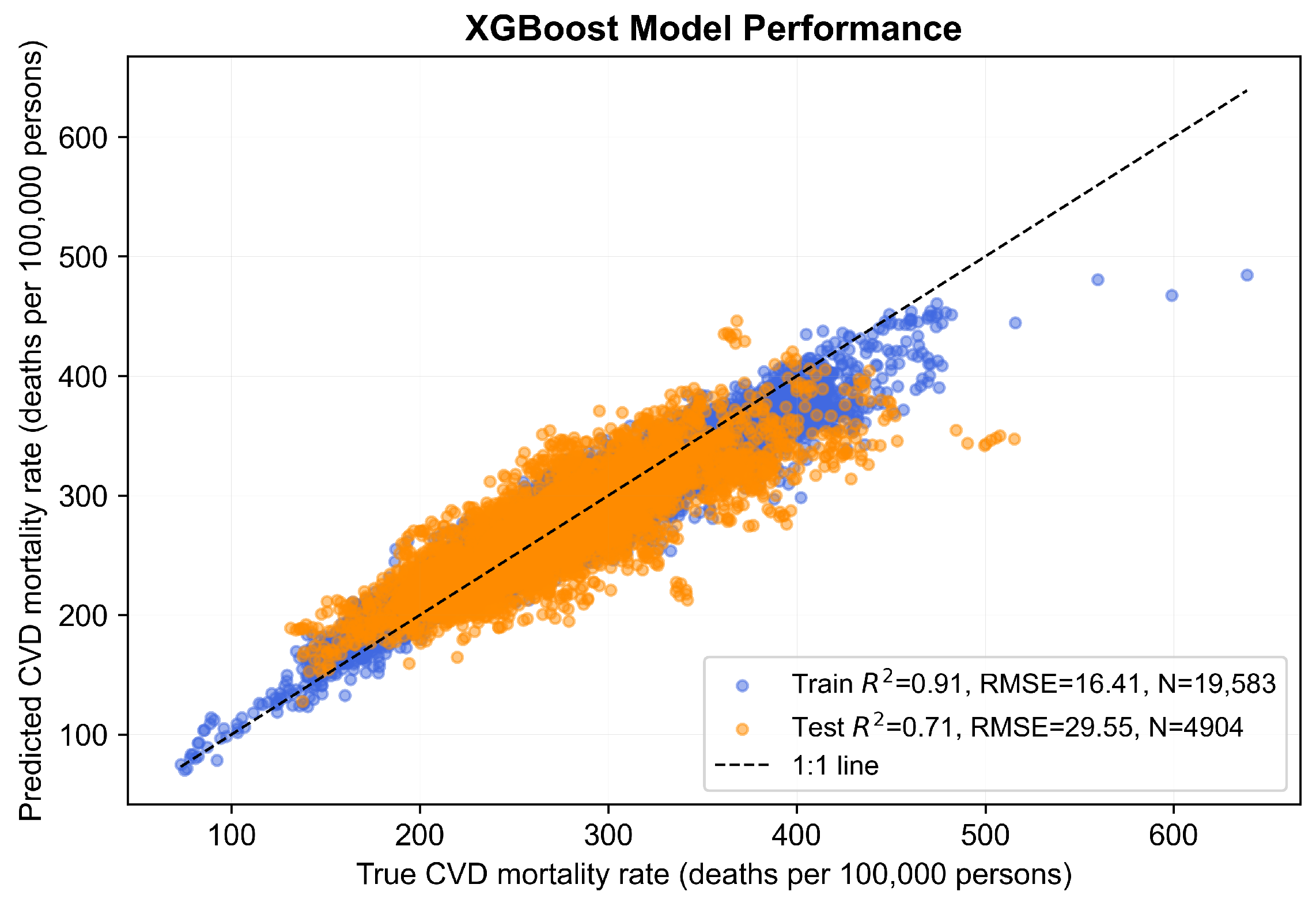
The full 43-feature model achieved a test R² of 0.706 and a test RMSE of 29.55 deaths per 100,000 persons, with a mean absolute error of 22.18 deaths per 100,000 persons on the held-out test set of 4904 county-year observations from 613 counties. The adjusted R² on the test set was 0.704, indicating that the result is not inflated by the number of predictors. On the training set, the model achieved R² = 0.911 and RMSE = 16.41 deaths per 100,000 persons across 19,583 county-year observations from 2448 counties. The gap between training and test R² was 0.205. All test counties were withheld from training, so test performance reflects prediction in counties not seen during model fitting. Predicted versus observed CVD mortality rates are shown in Figure 3.

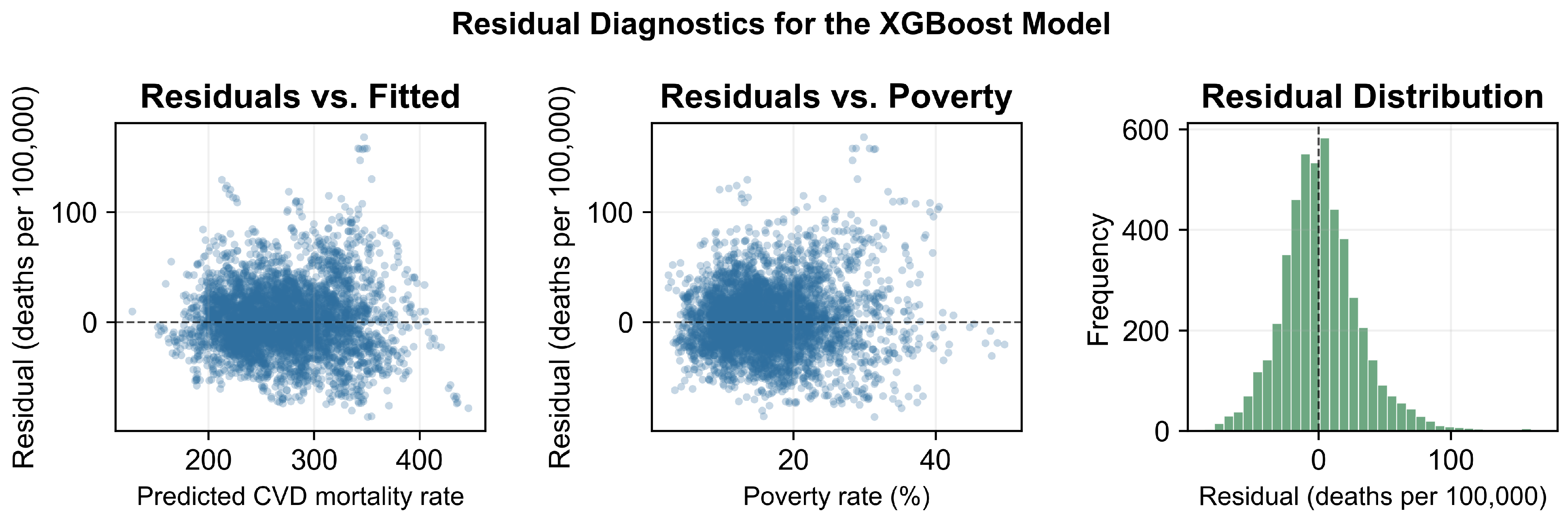
Residual diagnostics for the full 43-feature model are shown in Figure 4. Residuals were centered at zero across the full range of fitted values and showed no systematic relationship with poverty rate. The distribution of residuals was approximately normal. No directional bias was apparent at any level of predicted CVD mortality.

3.2. Feature Importance

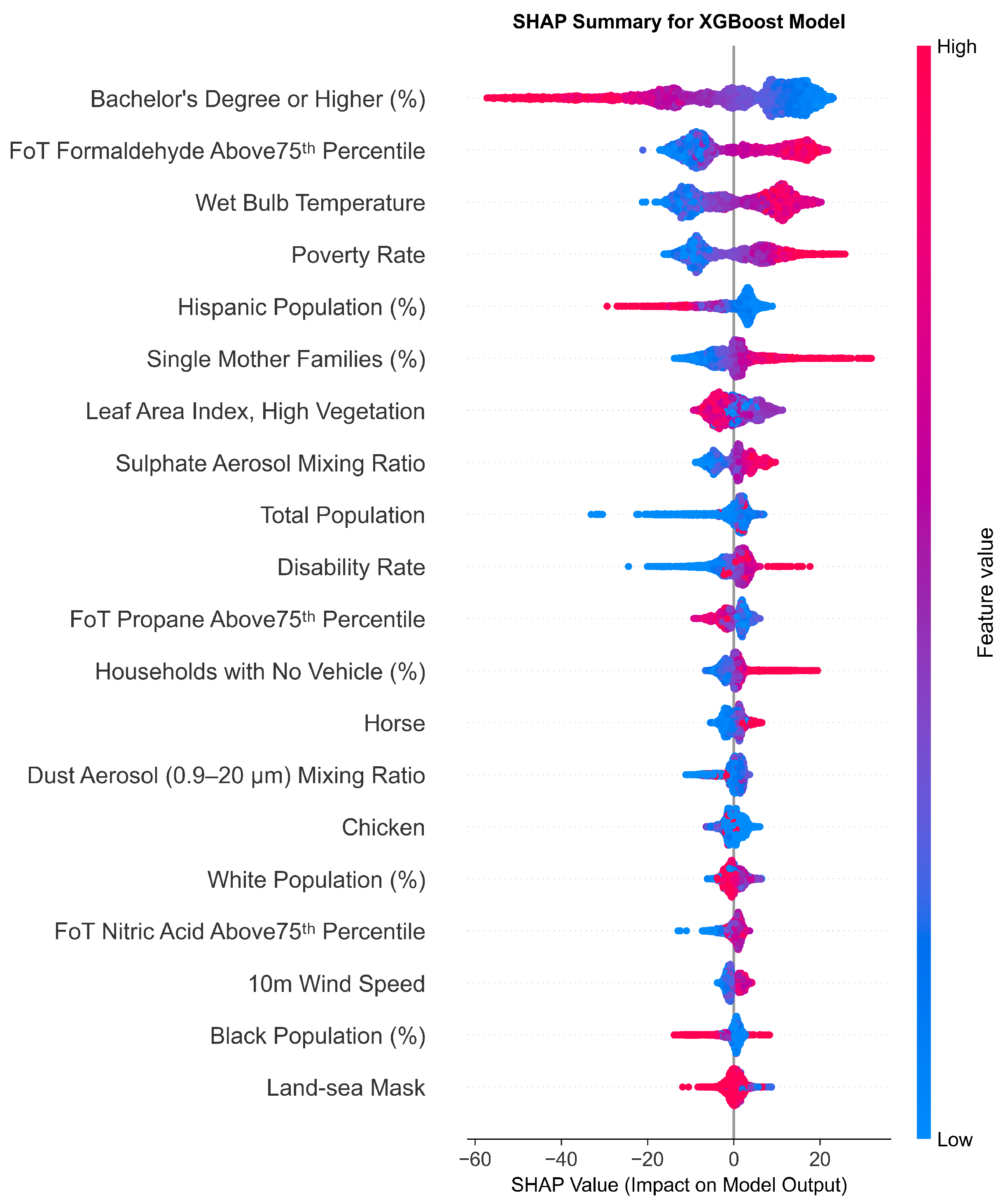
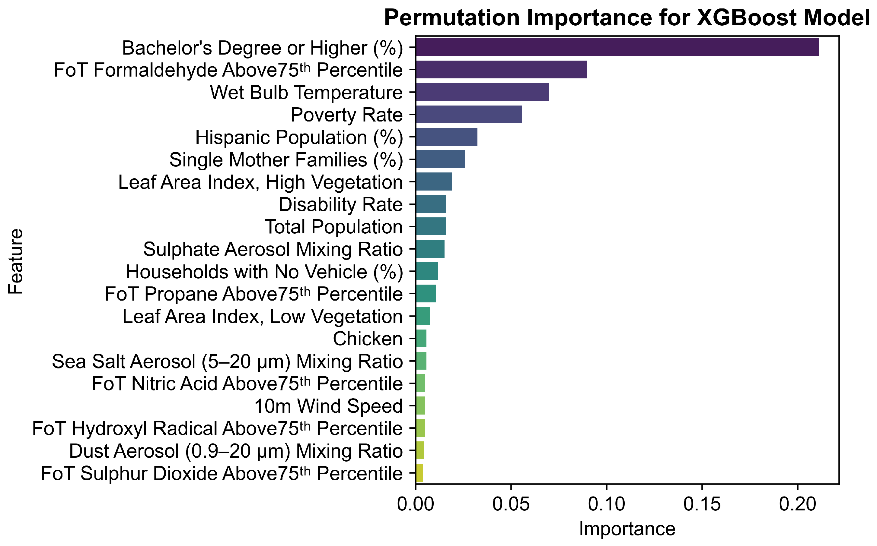
SHAP values were computed for all test-set predictions to rank predictors by their contribution to predicted CVD mortality. The SHAP beeswarm plot is shown in Figure 5. Permutation importance, computed independently on the test set, yielded consistent rankings for the top predictors (Figure 6).

The percentage of adults with a bachelor’s degree or higher (Bachelor’s Degree or Higher %) was the strongest predictor, with higher values associated with lower predicted CVD mortality. FoT Formaldehyde Above the 75th Percentile ranked second and Wet-bulb Temperature third. Both showed positive associations with predicted CVD mortality, with higher exposure corresponding to higher predicted mortality rates. Poverty Rate ranked fourth, with higher rates associated with higher predicted mortality. Among the top ten predictors, four were drawn from the CAMS/ERA5-derived predictor set (FoT Formaldehyde, Wet-bulb Temperature, Leaf Area Index for High Vegetation, and Sulphate Aerosol Mixing Ratio), four were socioeconomic, and two were demographic.

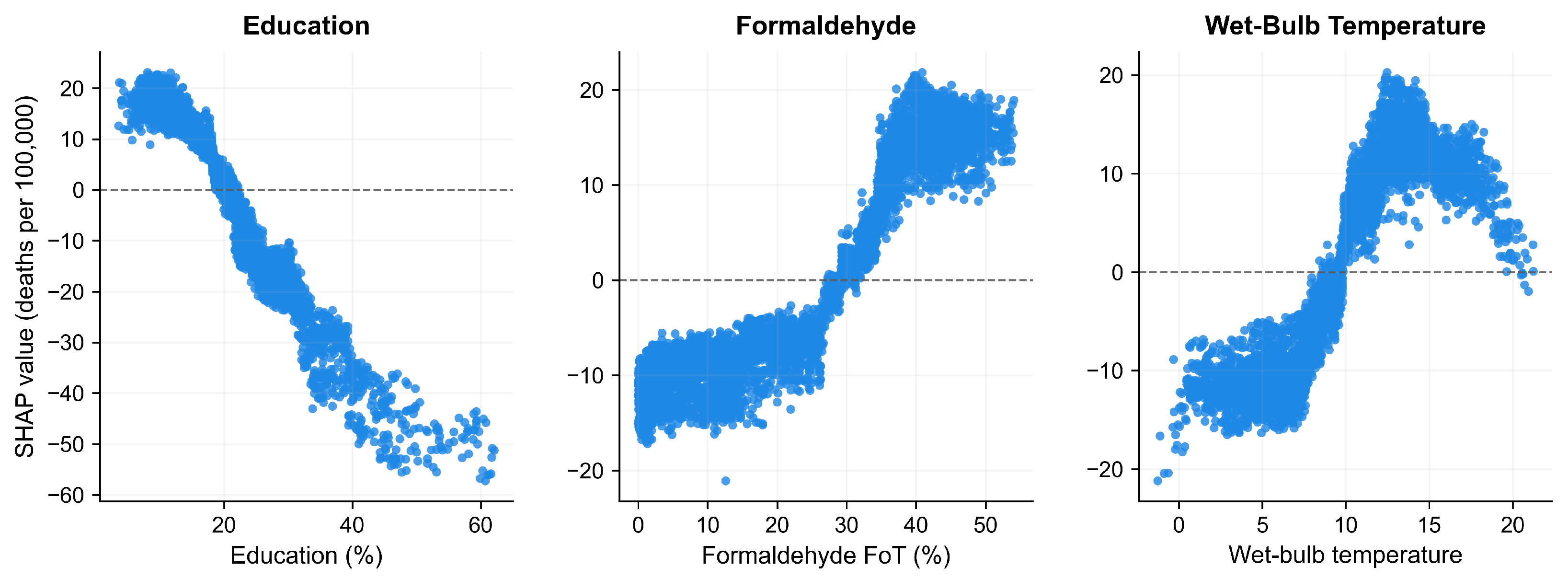
SHAP dependence plots for the three highest-ranked predictors are shown in Figure 7. Educational attainment showed a monotonic negative relationship with predicted CVD mortality. FoT Formaldehyde Above the 75th Percentile showed a positive SHAP pattern that steepened at higher exposure levels, consistent with a non-linear model response. Wet-bulb Temperature showed a positive association across its full observed range.

3.3. Feature Ablation Study

Table 3. Test-set performance across feature subsets. RMSE and MAE are expressed in deaths per 100,000 persons.

Feature Set	N	Test R2	Test Adj R2	Test RMSE	Test MAE
All features	43	0.706	0.704	29.55	22.18
Top 20	20	0.703	0.702	29.69	22.35
Top 10	10	0.679	0.678	30.90	22.98
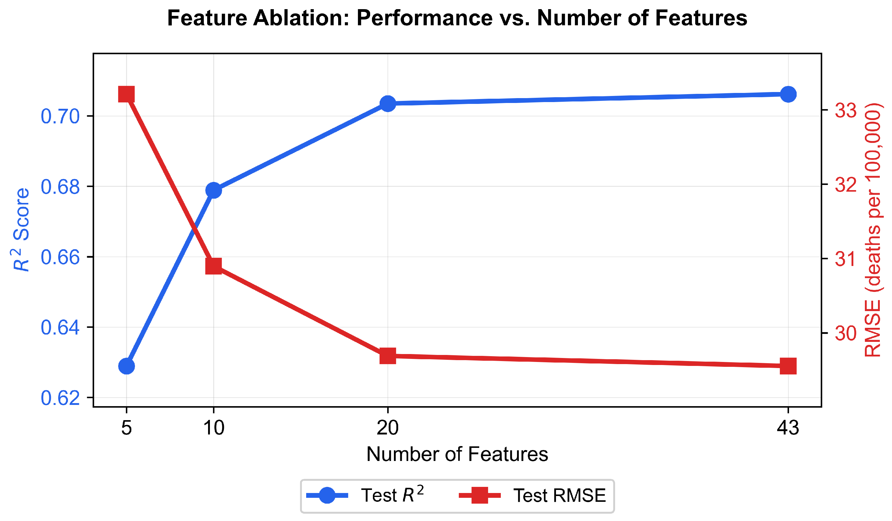
Top 5	5	0.629	0.629	33.21	25.04

summarizes test-set performance across all four feature subsets. The top-20 model achieved a test R² of 0.703 and a test RMSE of 29.69 deaths per 100,000 persons, a difference of 0.003 in R² from the full model while using fewer than half the predictors. The top-10 model reduced test R² to 0.679, a decline of 0.027 from the full model. The sharpest degradation occurred at the top-5 subset, where test R² fell to 0.629 and test RMSE rose to 33.21 deaths per 100,000 persons. Figure 8 shows that performance gains are concentrated in the transition from five to ten features, with diminishing returns above ten. The top 20 features provided similar performance to the full model, while further reduction below ten features resulted in meaningful performance loss.

3.4. Robustness and Validation Analyses

The CAMS grid diagnostic showed that the centroids of 3061 study counties fell within 1194 CAMS grid cells. Each grid cell contained a mean of 2.56 counties, a median of 2 counties, and a maximum of 11 counties. Polygon overlap showed that 2683 counties (87.7%) overlapped more than one CAMS grid cell, with a mean of 3.03 grid cells per county and a maximum of 20. In temporal validation, the model trained on 2012–2016 and tested on 2017–2019 achieved test R² = 0.788, RMSE = 25.34, and MAE = 18.99 deaths per 100,000 persons.

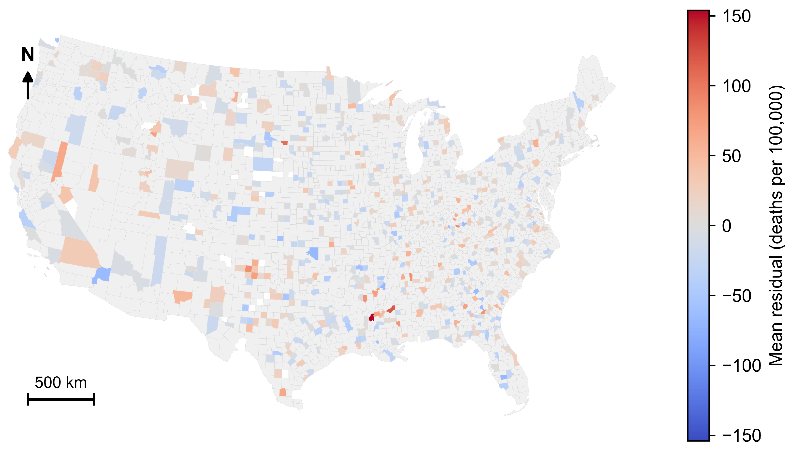
Formaldehyde ranking was stable across cross-validation folds. In five-fold GroupKFold validation, formaldehyde ranked second in all five folds. The mean cross-validation R² was 0.709, with mean RMSE = 29.51 and mean MAE = 22.10 deaths per 100,000 persons. Moran’s I for held-out county residuals was 0.061 ($z=3.30$, $p=0.001$), indicating a small but statistically significant degree of geographic clustering. Because Moran’s I ranges from $-1$ to $+1$, this value is close to zero and indicates weak residual spatial structure. The spatial distribution of held-out residuals is shown in Figure 9.

In the livestock sensitivity analysis, removing all seven livestock predictors changed test R² from 0.706 to 0.704 and RMSE from 29.55 to 29.69. Formaldehyde remained ranked second by SHAP importance.

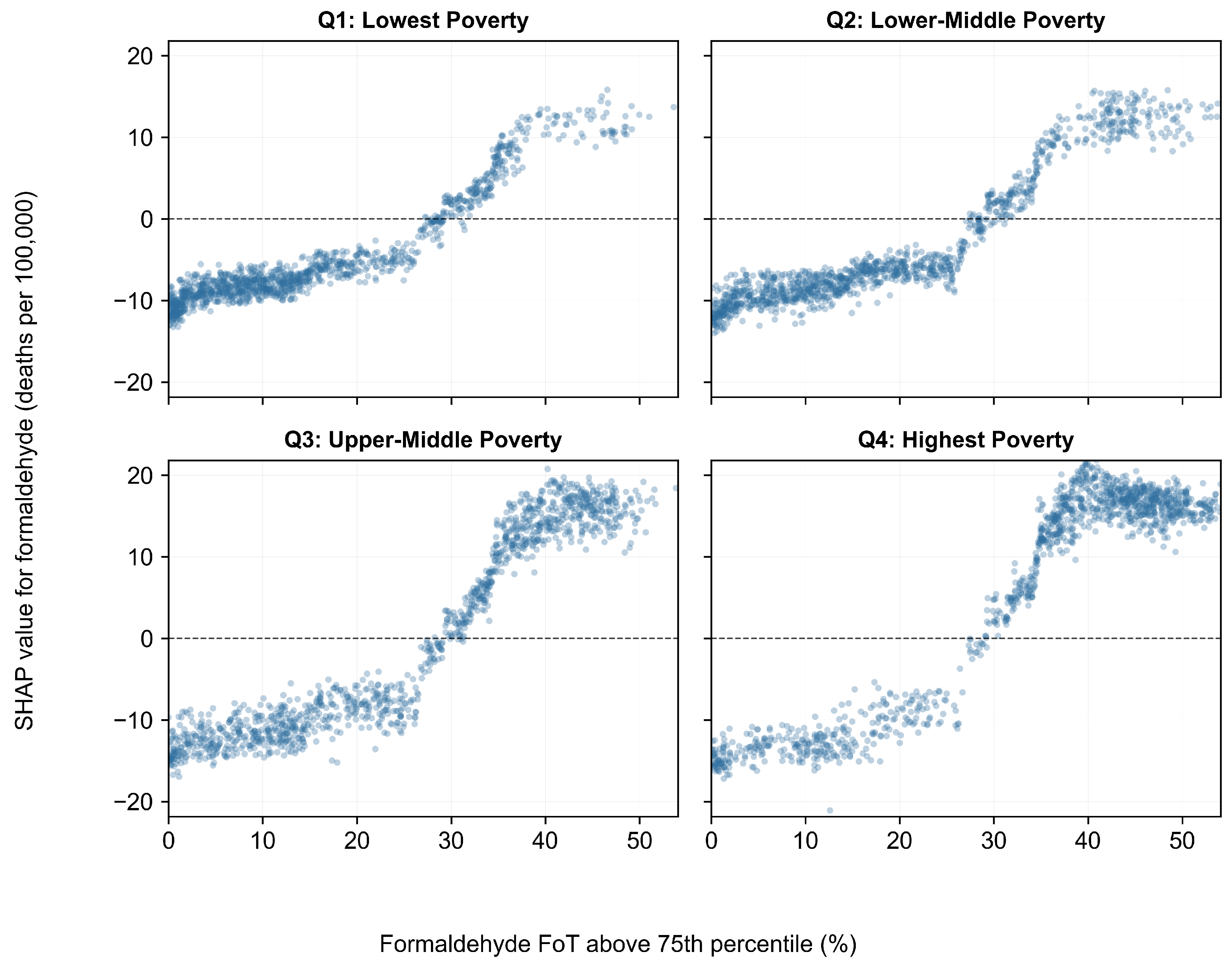
The formaldehyde-poverty analysis showed that formaldehyde SHAP values shifted upward across poverty quartiles. Formaldehyde SHAP was negative on average in the lowest-poverty quartile, with a mean of $-4.77$ deaths per 100,000 persons, and positive in the highest-poverty quartile, with a mean of $6.96$ deaths per 100,000 persons. The share of positive formaldehyde SHAP values increased from 20.8% to 70.4%. After controlling for poverty rate and bachelor’s degree attainment, the partial correlation between formaldehyde and CVD mortality was $r=0.474$ ($p<0.001$) for county-year observations and $r=0.477$ ($p<0.001$) for county means. The quartile-specific SHAP pattern is shown in Figure 10.

Model performance by Census region is shown in

Table 4. Held-out test performance by US Census region. RMSE and MAE are expressed in deaths per 100,000 persons.

Region	Test Counties	Test R2	Test RMSE	Test MAE
Northeast	43	0.495	20.08	15.30
Midwest	192	0.660	24.22	18.69
South	286	0.562	34.65	26.23
West	92	0.398	25.99	20.10

. Regional test R² ranged from 0.398 in the West to 0.660 in the Midwest.

4. Discussion

4.1. Atmospheric Predictors of County-Level CVD Mortality

FoT Formaldehyde Above the 75th Percentile ranked second, Wet-bulb Temperature ranked third, Leaf Area Index for High Vegetation ranked seventh, and Sulphate Aerosol Mixing Ratio ranked eighth among all 43 predictors by mean absolute SHAP value. These four predictors came from the CAMS/ERA5-derived predictor set. Each ranked above several socioeconomic or demographic predictors. This suggests that CAMS/ERA5 variables contain county-level prediction information that is not fully captured by poverty, education, or other socioeconomic predictors. Environmental exposures are recognized determinants of cardiovascular health through multiple biological pathways [7], but the rankings reported here should be read as predictive results, not as individual-level causal estimates.

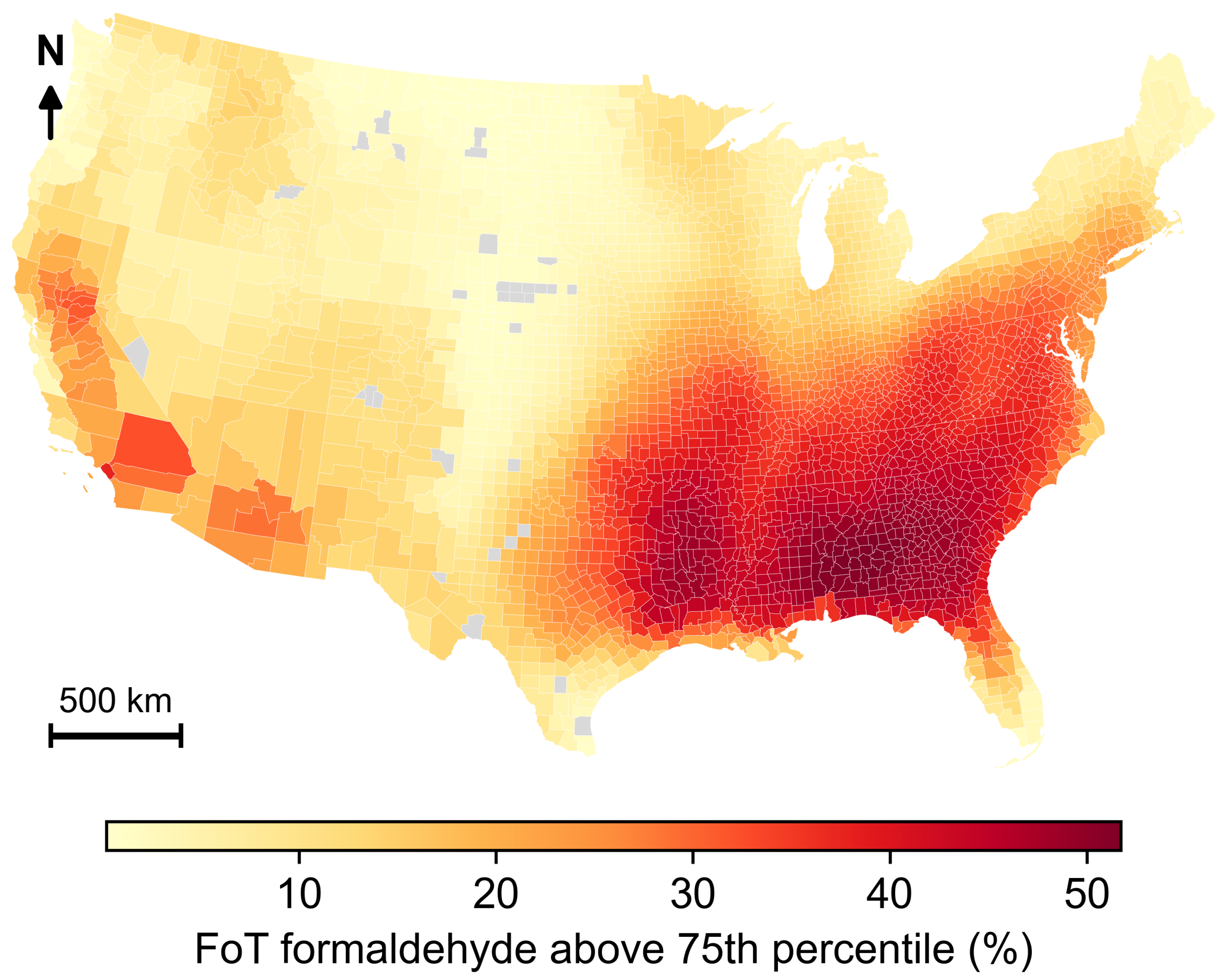
FoT Formaldehyde Above the 75th Percentile measures how often county-level formaldehyde values were higher than the dataset’s 75th percentile during a year. It is a measure of repeated high-exposure periods at the county level, not a measure of an individual person’s short-term exposure. Prior experimental evidence reports that formaldehyde exposure can affect cardiovascular biology through oxidative stress, endothelial dysfunction, and vascular inflammation [13]. At the population level, higher ambient formaldehyde concentrations have been associated with increased circulatory disease mortality across Chinese counties [14]. In the present model, counties with more frequent high-formaldehyde periods had higher predicted CVD mortality. This is consistent with prior evidence, but it does not show that formaldehyde exposure caused individual deaths. Figure 11 shows the geographic distribution of FoT Formaldehyde across US counties, averaged over 2012–2019, with the highest exposure frequencies concentrated in the Southeast and Gulf Coast, regions that also bear a high burden of cardiovascular disease mortality in the United States.

The formaldehyde-poverty analysis helps evaluate whether the formaldehyde result mainly reflected socioeconomic differences. Formaldehyde SHAP values shifted from negative in the lowest-poverty quartile to positive in the highest-poverty quartile, and the partial correlation remained positive after controlling for poverty rate and bachelor’s degree attainment. This suggests that formaldehyde added county-level prediction information beyond these socioeconomic variables.

When all seven livestock predictors were removed, formaldehyde remained ranked second by SHAP importance and test R² changed from 0.706 to 0.704. This suggests that the formaldehyde signal was not driven by shared variation with livestock density.

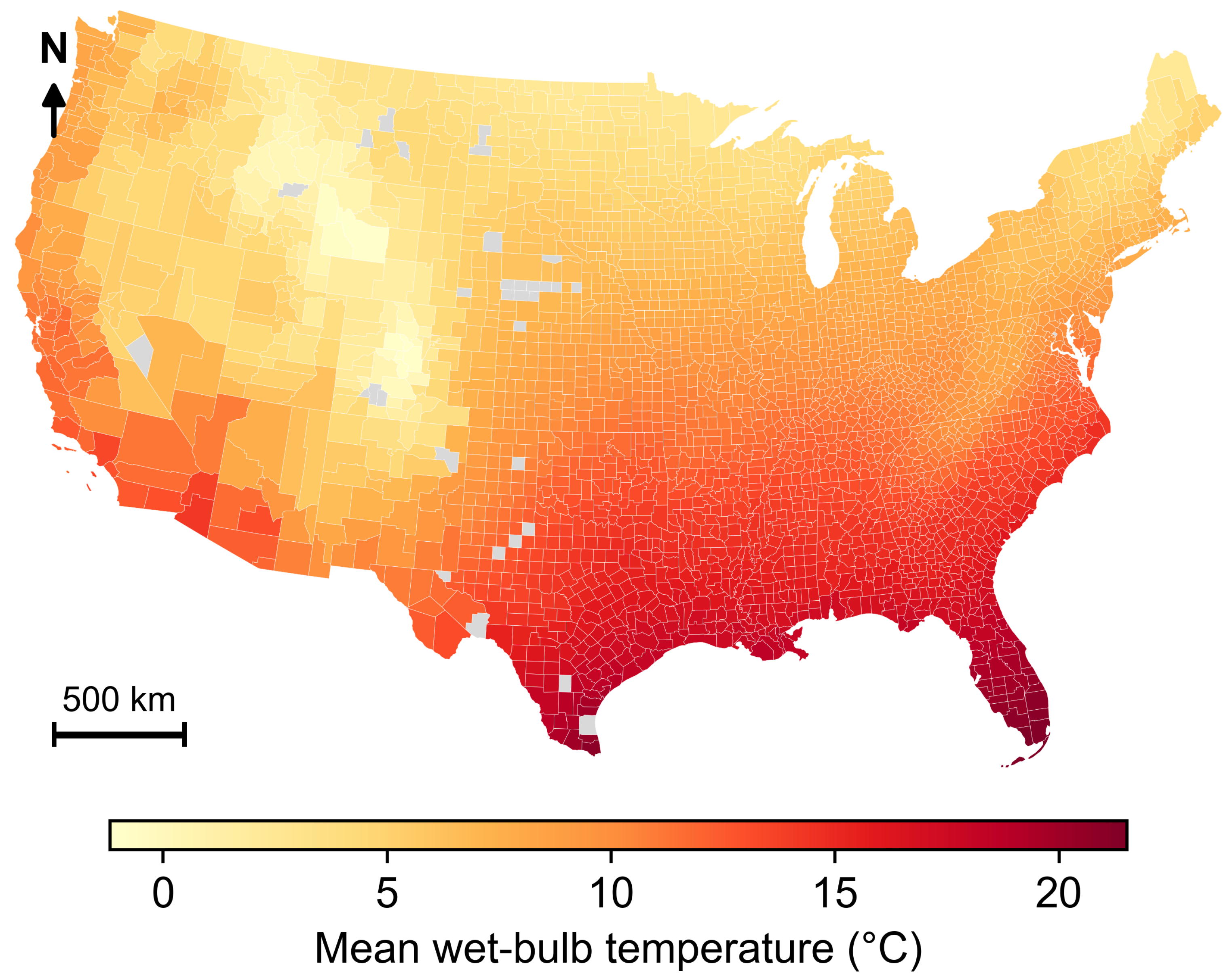
Wet-bulb temperature ranked third. Unlike dry-bulb temperature, wet-bulb temperature captures both heat and humidity, reflecting conditions under which the body cannot effectively dissipate heat through evaporation [15]. Heat stress increases cardiovascular strain because the body must raise cardiac output and shift blood flow toward the skin to maintain core temperature [7]. In people with existing coronary disease or reduced cardiac reserve, this added demand can increase the risk of myocardial ischemia and arrhythmia. Large studies show that many deaths linked to extreme temperatures involve cardiovascular causes [17] and that heat-related mortality is disproportionately cardiovascular in nature [29]. In the present model, counties with higher wet-bulb temperatures had higher predicted CVD mortality. Figure 12 shows the geographic distribution of mean wet-bulb temperature across US counties, with the highest values concentrated in the Gulf Coast and the Deep South.

Sulphate aerosol mixing ratio ranked eighth. Sulphates are a major component of fine particulate matter (PM_2.5), and long-term PM_2.5 exposure has been linked to higher cardiovascular mortality in large US population studies [30,31]. Among 53 million US Medicare beneficiaries, PM_2.5 was associated with elevated cardiovascular cause-specific mortality [10]. Because sulphate aerosol ranked highly while other atmospheric variables were also included, it may contain prediction information not fully captured by the other atmospheric variables in the model. This should be interpreted as a model result, not proof of a sulphate-specific causal effect.

Leaf Area Index for High Vegetation ranked seventh. This variable measures tree canopy density and likely captures geographic variation in land cover rather than a direct exposure pathway.

Livestock density should also be interpreted cautiously. Livestock density is not a direct cardiovascular exposure. It was included because animal operations can emit ammonia, methane, and nitrous oxide and can also mark broader agricultural land-use patterns. Any livestock-related signal should therefore be read as indirect regional context, not as evidence that livestock density directly affects CVD mortality.

Taken together, four of the top ten SHAP predictors came from the CAMS/ERA5-derived predictor set. The model results show that these variables add county-level prediction information beyond the socioeconomic predictors included in the model. They should be interpreted as geographic predictors, not as individual-level causal estimates.

4.2. Socioeconomic and Demographic Determinants

The percentage of adults with a bachelor’s degree or higher (Bachelor’s Degree or Higher %) ranked first among all 43 predictors, with higher county-level values associated with lower predicted CVD mortality. This is consistent with a large body of evidence linking population educational levels to cardiovascular outcomes [3,4]. At the county level, educational attainment correlates with income, occupational risk, healthcare access, and health behaviors, making it a compound indicator of socioeconomic conditions rather than a single pathway [6]. Poverty rate ranked fourth and showed a positive SHAP direction, consistent with the social determinants of health literature [32,33]. The two predictors are correlated but carry partially non-overlapping information, and the presence of both in the top five suggests that each adds prediction information to the model.

The percentage of Hispanic residents (Hispanic Population %) ranked fifth and showed a negative SHAP direction. Counties with larger Hispanic populations had lower predicted CVD mortality after accounting for socioeconomic and atmospheric covariates. This pattern is consistent with the Hispanic paradox, in which Hispanic adults in the United States have lower cardiovascular mortality than non-Hispanic White adults despite a less favorable socioeconomic profile [34]. Several explanations have been proposed, including healthy migrant effects, social support, diet, and cultural factors. The ACS variables used here do not capture nativity, immigration history, length of residence, or differences within the Hispanic population. Race and ethnicity misclassification on death certificates may also affect mortality estimates. For these reasons, this result should be read as a county-level demographic pattern, not as evidence that Hispanic ethnicity itself lowers individual CVD risk.

The percentage of single mother families (Single Mother Families %) ranked sixth, with a positive SHAP direction. This variable is best interpreted as a county-level marker of household and economic strain. It may reflect caregiver burden, housing instability, limited transportation, and reduced access to care, rather than a direct effect of household structure itself. This interpretation is consistent with evidence that single-parent household status is associated with elevated cardiovascular risk [35]. Disability Rate ranked tenth and also showed a positive SHAP direction.

4.3. Strengths and Limitations

This study has several methodological strengths. Model evaluation used geographic train–test separation by county FIPS code, so that every county in the test set was entirely absent from training. This design ensures that no county contributed observations to both the training and test sets, which is the appropriate holdout for data structured as repeated observations across counties and years. SHAP values were computed using TreeExplainer, which provides exact Shapley values rather than approximations, enabling reliable attribution of model predictions to individual features across the full predictor set. The predictor space spans socioeconomic, demographic, atmospheric, and land-surface domains, reflecting the multifactorial nature of county-level CVD mortality. The feature ablation study showed that predictive performance is distributed across the predictor set and is not driven by any single variable or small subset. Temporal validation, in which the model was trained on 2012–2016 and tested on 2017–2019, achieved test R² = 0.788 and RMSE = 25.34 deaths per 100,000 persons. This validation tested prediction across time, but the same counties could appear in both the training and test periods. The main test split is therefore the stronger test because it evaluates counties that were never used during model fitting.

Several limitations should be acknowledged. First, this is a county-level study. The model identifies geographic patterns in county averages. It does not estimate individual exposure, individual risk, or individual causal effects. A county can contain people with very different pollution exposures, occupations, diets, smoking histories, genetic risks, and access to clinical care. These individual-level factors were not measured and may partly explain the county-level patterns observed here. SHAP values identify which predictors contribute most to model predictions, but they do not establish whether those predictors cause CVD mortality.

Second, counties are imperfect spatial units. County averages can hide neighborhood-level inequality within the same county. Choropleth maps can also visually emphasize large-area counties, especially in the western United States, while smaller eastern counties are harder to see. The maps should therefore be read as geographic summaries, not as statements about all people within a county. Model performance also varied by Census region, with the lowest R² in the West (Table 4). Regional R² values should be read cautiously because each region contains fewer test counties than the national test set. They also reflect performance within that region only, not across the full national range of CVD mortality.

Third, the exposure data have spatial and measurement limits. Atmospheric data were drawn from CAMS/ERA5 reanalysis at 0.75° spatial resolution. At this resolution, county centroids mapped to CAMS cells with a mean of 2.56 counties per cell and a maximum of 11 counties per cell. Polygon overlap showed that 87.7% of counties overlapped more than one CAMS grid cell. This resolution is coarser than many US counties, especially in densely populated eastern states, so nearby counties may receive similar or identical atmospheric values. This spatial smoothing can mask local pollution gradients and may weaken county-level associations. GLW livestock density is estimated from livestock records and spatial models. It is not a direct count of animals in each county. Uncertainty in CAMS/ERA5 and GLW estimates can propagate into XGBoost predictions and SHAP rankings because the model uses these estimates as input data. Direct validation of the CAMS/ERA5 variables against ground monitors was outside the scope of this study. Future work should compare reanalysis estimates with independent ground observations where available and test higher-resolution exposure products or statistical downscaling.

Fourth, each county-year is treated as an independent observation. The model does not track how conditions within individual counties change from year to year. Whether the model relationships documented here persist or change as environmental and socioeconomic conditions evolve cannot be determined from this analysis alone. A Moran’s I test applied to held-out test residuals found weak but statistically significant spatial structure (Moran’s I = 0.061, $z=3.30$, $p=0.001$). This suggests that prediction errors were weakly clustered among nearby counties. Future work could apply spatial regression models to account for this structure directly.

5. Conclusions

An XGBoost model trained on 43 county-level predictors explained 70.6% of the variance in cardiovascular disease mortality across US counties (Test R² = 0.706, RMSE = 29.55 per 100,000 persons). Four of the top ten predictors by SHAP value came from CAMS/ERA5. FoT Formaldehyde Above the 75th Percentile ranked second, Wet-bulb Temperature ranked third, Leaf Area Index for High Vegetation ranked seventh, and Sulphate Aerosol Mixing Ratio ranked eighth. These variables added county-level prediction information beyond the socioeconomic variables included in the model.

CAMS/ERA5 data may complement socioeconomic indicators in county-level CVD surveillance. These data can help identify counties where additional monitoring, environmental assessment, or public health planning may be useful. The results should not be interpreted as identifying individual causal risk. Formaldehyde, wet-bulb temperature, sulphate aerosol, and leaf-area measures are routinely available from satellite and reanalysis products, so they can be incorporated into geographic surveillance workflows. Future work should test finer-resolution exposure data, compare reanalysis estimates with ground observations, and examine how these county-level patterns change over time.

References

1. Martin, S.S.; Aday, A.W.; Allen, N.B.; Almarzooq, Z.I.; Anderson, C.A.M.; Arora, P.; Avery, C.L.; Baker-Smith, C.M.; Bansal, N.; Beaton, A.Z.; et al. 2025 Heart Disease and Stroke Statistics: A Report of US and Global Data From the American Heart Association. Circulation 2025, 151, e41–e660. [Google Scholar] [CrossRef] [PubMed]
2. Roth, G.A.; Dwyer-Lindgren, L.; Bertozzi-Villa, A.; Stubbs, R.W.; Morozoff, C.; Naghavi, M.; Mokdad, A.H.; Murray, C.J.L. Trends and Patterns of Geographic Variation in Cardiovascular Mortality Among US Counties, 1980–2014. JAMA 2017, 317, 1976–1992. [Google Scholar] [CrossRef] [PubMed]
3. Havranek, E.P.; Mujahid, M.S.; Barr, D.A.; Blair, I.V.; Cohen, M.S.; Cruz-Flores, S.; Davey-Smith, G.; Dennison-Himmelfarb, C.R.; Lauer, M.S.; Lockwood, D.W.; et al. Social Determinants of Risk and Outcomes for Cardiovascular Disease: A Scientific Statement From the American Heart Association. Circulation 2015, 132, 873–898. [Google Scholar] [CrossRef] [PubMed]
4. Schultz, W.M.; Kelli, H.M.; Lisko, J.C.; Varghese, T.; Shen, J.; Sandesara, P.; Quyyumi, A.A.; Taylor, H.A.; Gulati, M.; Harold, J.G.; et al. Socioeconomic Status and Cardiovascular Outcomes: Challenges and Interventions. Circulation 2018, 137, 2166–2178. [Google Scholar] [CrossRef] [PubMed]
5. Pampel, F.C.; Krueger, P.M.; Denney, J.T. Socioeconomic Disparities in Health Behaviors. Annu. Rev. Sociol. 2010, 36, 349–370. [Google Scholar] [CrossRef] [PubMed]
6. Zajacova, A.; Lawrence, E.M. The relationship between education and health: Reducing disparities through a contextual approach. Annu. Rev. Public Health 2018, 39, 273–289. [Google Scholar] [CrossRef] [PubMed]
7. Blaustein, J.R.; Quisel, M.J.; Hamburg, N.M.; Wittkopp, S. Environmental Impacts on Cardiovascular Health and Biology: An Overview. Circ. Res. 2024, 134, 1048–1060. [Google Scholar] [CrossRef] [PubMed]
8. Kelly, F.J.; Fussell, J.C. Air pollution and public health: Emerging hazards and improved understanding of risk. Environ. Geochem. Health 2015, 37, 631–649. [Google Scholar] [CrossRef] [PubMed]
9. Manisalidis, I.; Stavropoulou, E.; Stavropoulos, A.; Bezirtzoglou, E. Environmental and Health Impacts of Air Pollution: A Review. Front. Public Health 2020, 8, 14. [Google Scholar] [CrossRef] [PubMed]
10. Wang, B.; Eum, K.D.; Kazemiparkouhi, F.; Li, C.; Manjourides, J.; Pavlu, V.; Suh, H.H. The impact of long-term PM2.5 exposure on specific causes of death: Exposure-response curves and effect modification among 53 million U.S. Medicare beneficiaries. Environ. Health 2020, 19, 20. [Google Scholar] [CrossRef] [PubMed]
11. Sethi, Y.; Mehta, S.; Padda, I.; Marlecha, P.; Moinuddin, A. Impact of PM2.5 Exposure on Cardiovascular Diseases (IPEC Study): An Updated Umbrella Review of Systematic Reviews and Meta-Analyses. Eur. J. Prev. Cardiol. 2026, zwag005. [Google Scholar] [CrossRef] [PubMed]
12. Ghelli, F.; Bellisario, V.; Squillacioti, G.; Panizzolo, M.; Santovito, A.; Bono, R. Formaldehyde in Hospitals Induces Oxidative Stress: The Role of GSTT1 and GSTM1 Polymorphisms. Toxics 2021, 9, 178. [Google Scholar] [CrossRef] [PubMed]
13. Zhang, Y.; Yang, Y.; He, X.; Yang, P.; Zong, T.; Sun, P.; Sun, R.C.; Yu, T.; Jiang, Z. The cellular function and molecular mechanism of formaldehyde in cardiovascular disease and heart development. J. Cell. Mol. Med. 2021, 25, 5358–5371. [Google Scholar] [CrossRef] [PubMed]
14. Ban, J.; Su, W.; Zhong, Y.; Liu, C.; Li, T. Ambient formaldehyde and mortality: A time series analysis in China. Sci. Adv. 2022, 8, eabm4097. [Google Scholar] [CrossRef] [PubMed]
15. Raymond, C.; Matthews, T.; Horton, R.M. The emergence of heat and humidity too severe for human tolerance. Sci. Adv. 2020, 6, eaaw1838. [Google Scholar] [CrossRef] [PubMed]
16. Crouse, D.L.; Peters, P.A.; Hystad, P.; Brook, J.R.; van Donkelaar, A.; Martin, R.V.; Villeneuve, P.J.; Jerrett, M.; Goldberg, M.S.; Pope, C.A., III; et al. Ambient PM2.5, O3, and NO2 exposures and associations with mortality over 16 years of follow-up in the Canadian Census Health and Environment Cohort (CanCHEC). Environ. Health Perspect. 2015, 123, 1180–1186. [Google Scholar] [CrossRef] [PubMed]
17. Zhao, Q.; Guo, Y.; Ye, T.; Gasparrini, A.; Tong, S.; Overcenco, A.; Urban, A.; Schneider, A.; Entezari, A.; Vicedo-Cabrera, A.M.; et al. Global, regional, and national burden of mortality associated with non-optimal ambient temperatures from 2000 to 2019: A three-stage modelling study. Lancet Planet. Health 2021, 5, e415–e425. [Google Scholar] [CrossRef] [PubMed]
18. Zhu, L.; Jacob, D.J.; Keutsch, F.N.; Mickley, L.J.; Scheffe, R.D.; Strum, M.; González Abad, G.; Chance, K.; Yang, K.; Rappenglück, B.; et al. Formaldehyde (HCHO) as a Hazardous Air Pollutant: Mapping Surface Air Concentrations from Satellite and Inferring Cancer Risks in the United States. Environ. Sci. Technol. 2017, 51, 5650–5657. [Google Scholar] [CrossRef] [PubMed]
19. Wang, P.; Holloway, T.; Bindl, M.; Harkey, M.; De Smedt, I. Ambient Formaldehyde over the United States from Ground-Based (AQS) and Satellite (OMI) Observations. Remote Sens. 2022, 14, 2191. [Google Scholar] [CrossRef]
20. Chen, T.; Guestrin, C. XGBoost: A scalable tree boosting system. In Proceedings of the 22nd ACM SIGKDD International Conference on Knowledge Discovery and Data Mining; ACM: New York, NY, USA, 2016; pp. 785–794. [Google Scholar]
21. Lundberg, S.M.; Lee, S.I. A Unified Approach to Interpreting Model Predictions. arXiv 2017, arXiv:1705.07874. [Google Scholar] [CrossRef]
22. Wild Tree Tech; Google Brain; University of Liège; Saarland University. Scikit-Optimize: Sequential Model-Based Optimization in Python Version 0.8.1. 2020. Available online: https://scikit-optimize.github.io/stable/modules/generated/skopt.BayesSearchCV.html (accessed on 15 June 2026).
23. Institute for Health Metrics and Evaluation (IHME). United States Mortality Rates by Causes of Death and Life Expectancy by County, Race, and Ethnicity 2000–2019. Global Health Data Exchange (GHDx). 2023. Available online: https://ghdx.healthdata.org/record/ihme-data/united-states-causes-death-life-expectancy-by-county-race-ethnicity-2000-2019 (accessed on 15 June 2026).
24. U.S. Census Bureau. American Community Survey 5-Year Data (2009–2023). 2024. Available online: https://www.census.gov/data/developers/data-sets/acs-5year.html (accessed on 14 January 2026).
25. Inness, A.; Ades, M.; Agustí-Panareda, A.; Barré, J.; Benedictow, A.; Blechschmidt, A.M.; Dominguez, J.J.; Engelen, R.; Eskes, H.; Flemming, J.; et al. The CAMS reanalysis of atmospheric composition. Atmos. Chem. Phys. 2019, 19, 3515–3556. [Google Scholar] [CrossRef]
26. Gilbert, M.; Nicolas, G.; Cinardi, G.; Van Boeckel, T.P.; Vanwambeke, S.O.; Wint, G.W.; Robinson, T.P. Global distribution data for cattle, buffaloes, horses, sheep, goats, pigs, chickens and ducks in 2010. Sci. Data 2018, 5, 180227. [Google Scholar] [CrossRef] [PubMed]
27. Anestis, V.; Umar, W.; Dragoni, F.; van der Weerden, T.J.; Hassouna, M.; Noble, A.; Bartzanas, T.; Amon, B. Mitigation of greenhouse gas and ammonia emissions due to livestock housing management practices: Analysis of the DATAMAN database. Biosyst. Eng. 2025, 258, 104260. [Google Scholar] [CrossRef]
28. Moran, P.A.P. Notes on Continuous Stochastic Phenomena. Biometrika 1950, 37, 17–23. [Google Scholar] [CrossRef]
29. Gallo, E.; Quijal-Zamorano, M.; Méndez Turrubiates, R.F.; Tonne, C.; Basagaña, X.; Achebak, H.; Ballester, J. Heat-related mortality in Europe during 2023 and the role of adaptation in protecting health. Nat. Med. 2024, 30, 3101–3105. [Google Scholar] [CrossRef] [PubMed]
30. Pope, C.A., III; Ezzati, M.; Dockery, D.W. Fine-Particulate Air Pollution and Life Expectancy in the United States. N. Engl. J. Med. 2009, 360, 376–386. [Google Scholar] [CrossRef] [PubMed]
31. Di, Q.; Wang, Y.; Zanobetti, A.; Wang, Y.; Koutrakis, P.; Choirat, C.; Dominici, F.; Schwartz, J.D. Air Pollution and Mortality in the Medicare Population. N. Engl. J. Med. 2017, 376, 2513–2522. [Google Scholar] [CrossRef] [PubMed]
32. Marmot, M. Social determinants of health inequalities. Lancet 2005, 365, 1099–1104. [Google Scholar] [CrossRef] [PubMed]
33. Singh, G.K.; Lee, H. Marked Disparities in Life Expectancy by Education, Poverty Level, Occupation, and Housing Tenure in the United States, 1997–2014. Int. J. MCH AIDS 2021, 10, 7–18. [Google Scholar] [CrossRef] [PubMed]
34. Khan, S.U.; Lone, A.N.; Yedlapati, S.H.; Dani, S.S.; Khan, M.Z.; Watson, K.E.; Parwani, P.; Rodriguez, F.; Cainzos-Achirica, M.; Michos, E.D. Cardiovascular Disease Mortality Among Hispanic Versus Non-Hispanic White Adults in the United States, 1999 to 2018. J. Am. Heart Assoc. 2022, 11, e022857. [Google Scholar] [CrossRef] [PubMed]
35. Borrowman, J.D.; Pageau, L.M.; Cameron, N.A.; Carnethon, M.R.; Fields, N.D. Cardiovascular Health of Single Mothers: A Systematic Review. J. Am. Heart Assoc. 2025, 14, e043296. [Google Scholar] [CrossRef] [PubMed]
36. MI3NTS Research Group. Predicting CVD: Code and Processed Data. GitHub. 2026. Available online: https://github.com/mi3nts/predicting-cvd (accessed on 15 June 2026).
37. Copernicus Atmosphere Monitoring Service. CAMS Global Reanalysis (EAC4). Copernicus Atmosphere Data Store. 2026. Available online: https://ads.atmosphere.copernicus.eu/datasets/cams-global-reanalysis-eac4 (accessed on 15 June 2026).
38. Copernicus Climate Change Service. ERA5 Hourly Data on Single Levels from 1940 to Present. Copernicus Climate Data Store. 2026. Available online: https://cds.climate.copernicus.eu/datasets/reanalysis-era5-single-levels (accessed on 15 June 2026).
39. Food and Agriculture Organization of the United Nations. Gridded Livestock of the World: Global Distributions. FAO Livestock Systems. 2026. Available online: https://www.fao.org/livestock-systems/global-distributions/en/ (accessed on 15 June 2026).
40. Anthropic. Claude Sonnet 4.6. 2026. Available online: https://www.anthropic.com/news/claude-sonnet-4-6 (accessed on 15 June 2026).
41. OpenAI. Codex. 2026. Available online: https://developers.openai.com/codex/ (accessed on 15 June 2026).
42. Google. Gemini 3.1 Pro Preview. 2026. Available online: https://statics.teams.cdn.office.net/evergreen-assets/safelinks/2/atp-safelinks.html (accessed on 15 June 2026).
Figure 1. County-level age-standardized cardiovascular disease (CVD) mortality rate in the United States (2019). Grey counties indicate missing data.
Aisens 02 00008 g001
Figure 2. Study workflow.
Aisens 02 00008 g002
Figure 3. Predicted versus observed age-standardized CVD mortality rates (deaths per 100,000 persons) on the held-out test set (n = 4904 county-year observations). The dashed line indicates perfect agreement.
Aisens 02 00008 g003
Figure 4. Residual diagnostics for the full 43-feature model. (Left): residuals versus fitted values. (Center): residuals versus poverty rate. (Right): distribution of residuals. All residuals are in deaths per 100,000 persons.
Aisens 02 00008 g004
Figure 5. SHAP beeswarm plot for the full 43-feature model. Each row represents one predictor. Each point represents one test-set observation. Point color indicates the feature value (red = high, blue = low). Horizontal position indicates the direction and magnitude of each feature’s contribution to the predicted CVD mortality rate.
Aisens 02 00008 g005
Figure 6. Permutation importance for the full 43-feature model. Each bar shows the mean decrease in test R2 when the predictor’s values are randomly shuffled. The ranking is consistent with the SHAP analysis.
Aisens 02 00008 g006
Figure 7. SHAP dependence plots for the three highest-ranked predictors: Bachelor’s Degree or Higher % (left), FoT Formaldehyde Above the 75th Percentile (middle), and Wet-bulb Temperature (right). The x-axis shows the feature value. The y-axis shows the SHAP value (contribution to predicted CVD mortality). Point color encodes the value of the most interacting feature identified by SHAP.
Aisens 02 00008 g007
Figure 8. Ablation curve showing test R2 (left axis) and test RMSE (right axis) as a function of the number of predictors retained. Each point corresponds to a model trained on the top k features ranked by SHAP importance.
Aisens 02 00008 g008
Figure 9. Mean residuals for held-out test counties. Residuals are observed minus predicted CVD mortality rate, in deaths per 100,000 persons. Red counties indicate underprediction, blue counties indicate overprediction, and light grey counties are in the training set.
Aisens 02 00008 g009
Figure 10. Formaldehyde SHAP values by poverty quartile in the held-out test set. The x-axis shows county-level FoT Formaldehyde Above the 75th Percentile. The y-axis shows the SHAP contribution to predicted CVD mortality in deaths per 100,000 persons. The dashed horizontal line marks zero contribution.
Aisens 02 00008 g010
Figure 11. County-level mean FoT Formaldehyde Above the 75th Percentile across the contiguous United States, averaged over 2012–2019. Values represent the percentage of 3-hourly time steps in a year during which county-level formaldehyde concentrations exceeded the 75th percentile threshold of the full dataset. Grey counties indicate missing data.
Aisens 02 00008 g011
Figure 12. County-level mean wet-bulb temperature (°C) across the contiguous United States, averaged over 2012–2019. Wet-bulb temperature reflects the combined physiological burden of heat and humidity, representing conditions under which evaporative cooling is limited. Grey counties indicate missing data.
Aisens 02 00008 g012