Development of a Spatial Methodology for Minimum Temperature Estimation for Early Frost Management in Agricultural Areas of Central Macedonia ^†

Abstract

This research develops a reliable methodology for estimating minimum temperature distribution in agricultural areas, focusing on frost conditions threatening crop production. The data was collected across the plain of Krya Vrysi in Central Macedonia. The approach uses linear regression equations between daily minimum temperatures from a central station and 12 autonomous temperature sensors with data loggers. Statistical analysis covered winter 2023–2024, with 2025 validation showing exceptional predictive capability—R² values of 0.97–0.99 and RMSE of 0.34–0.58 °C. Spatial interpolation employed the Radial Basis Function with thin plate splines, effective for agricultural microclimatic interpolation. This methodology provides an operational frost prediction tool, enabling targeted interventions, reducing production losses and enhancing agricultural resilience.

1. Introduction

Frequently, in agricultural regions, the network of surface meteorological stations is sparse, a phenomenon attributed to the high cost of installation and maintenance of their equipment. Specifically, the insufficient availability of meteorological data utilized in local-scale crop models, which originate from stations installed at considerable distances from these areas, leads to unreliable predictions of meteorological conditions [1]. It is emphasized that these models could constitute the foundation for issuing agricultural warnings at the local level, upon which decisions are made for the rational planning of cultivation techniques [2] required for the protection of plant production.

Local-scale air temperature variations can alter the biological cycle of crops and their vulnerability to extreme conditions, such as frost and high-temperature episodes. Particularly during autumn, winter, and early spring periods, frosts, depending on their intensity, cause damage to field and tree crops both during the pre-flowering stage and later during flowering and fruit development [3]. This leads to a dramatic reduction in agricultural production and consequently to enormous economic losses [4], with implications for the national economy of states. Focusing on Greek territory, compensation paid due to frost damage to plant capital during the decade 2014–2023 amounted to 25% of the total sum disbursed by the Hellenic Organization of Agricultural Insurances (H.O.A.I.) [5] for all extreme weather phenomena, causing serious impacts on the country’s national income.

Accurate estimation of the spatial distribution of air temperature at local scale constitutes a significant tool in the planning of cultivation techniques [6,7]. It is noted that spatial interpolation techniques have been applied in the past, including regression methods, smoothing splines, inverse distance weighting, and kriging models [8,9,10,11,12]. However, geostatistical techniques based on data grid modelling have been recently employed [1].

This work aims to develop a real-time minimum temperature prediction model for the fertile plain of Krya Vrysi, Pella, employing spatial interpolation techniques while incorporating data from an automatic telemetric reference meteorological station in combination with data from autonomous recording instruments.

2. Materials and Methods

This research aims to develop a real-time minimum temperature prediction model for the fertile plain of Krya Vrysi in Pella through spatial interpolation techniques, incorporating data from an autonomous telemetric reference meteorological station. The development of the model was structured in four steps:

2.1. Step 1: Regression Equations Using Past Temperature Data

For the first step of the model development, we incorporated past years data (2023–2024) from twelve autonomous temperature sensors (Temperature/RH Smart Sensor, S-THC-M00x mounted in solar Radiation shield RS3-B, Onset Computer Corporation U.S.A.) with data loggers (Data Logger HOBO Micro Station, H21-USB, Onset Computer Corporation, MA, U.S.A.), placed at representative locations within the study area, in conjunction with the respective data of the reference station (the station is equipped with HD33M.2 data logger with an integrated GSM/GPRS module for data transmitting). Using data from the reference station and the data loggers, linear regression equations were developed to model their interrelationships. This set of regression equations was used to estimate the minimum temperature at the data logger sites depending on the temperature of the reference station.

2.2. Step 2: Evaluation of Prediction Accuracy

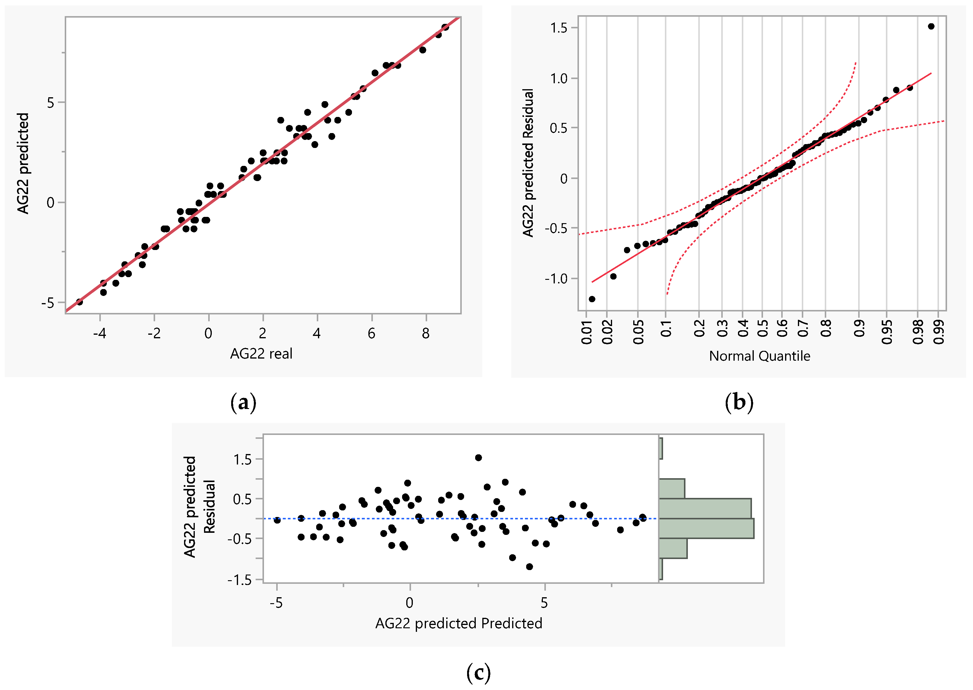
The degree of correlation between the predicted and the actual values was exceptionally high, with R² values ranging from 0.98 to 0.99 and RMSE values from 0.35 to 0.60. A graphical examination of the residuals was also conducted, which confirmed the suitability of the regression equations. As an example, the diagrams for site AG22 (with coordinates 40.7080, 22.3358) are presented in Figure 1, showing the linear correlation between estimated values and actual values (with R² = 0.98 and RMSE = 0.47) and the residual plot against estimated values. To test the normality of residuals, a Residual Normal Quantile Plot was employed.

2.3. Step 3: Spatial Interpolation of Minimum Temperatures Across the Entire Study Area

For spatial interpolation of the data, the Radial Basis Function (RBF) method was employed, which has proven particularly effective for interpolating microclimatic data in agricultural areas [13,14]. The Radial Basis Function (RBF) method is a spatial interpolation technique for calculating values at points without data, based on known values from neighbouring points. This method is widely used in geostatistics, geography, and other scientific fields where the prediction of continuous values from data at limited points is required. According to RBF theory, the value at an unknown point is calculated through functions and depends on its Euclidean distance from known reference points [15].

During method implementation, evaluation of linear, cubic, gaussian, and thin plate splines (TPS) kernels were conducted, with the TPS kernel selected as most suitable due to its ability to combine estimation accuracy with smoothness in temperature maps [16].

The developed frost risk estimation model consequently combines regression equations with spatial interpolation for estimating minimum temperature values across the entire study area from single base station data. Spatial analysis was performed with 0.001° latitude/longitude resolution, corresponding to approximately 111 m for the examined region.

2.4. Step 4: Validation of Spatial Interpolation Using Independent Temperature Data

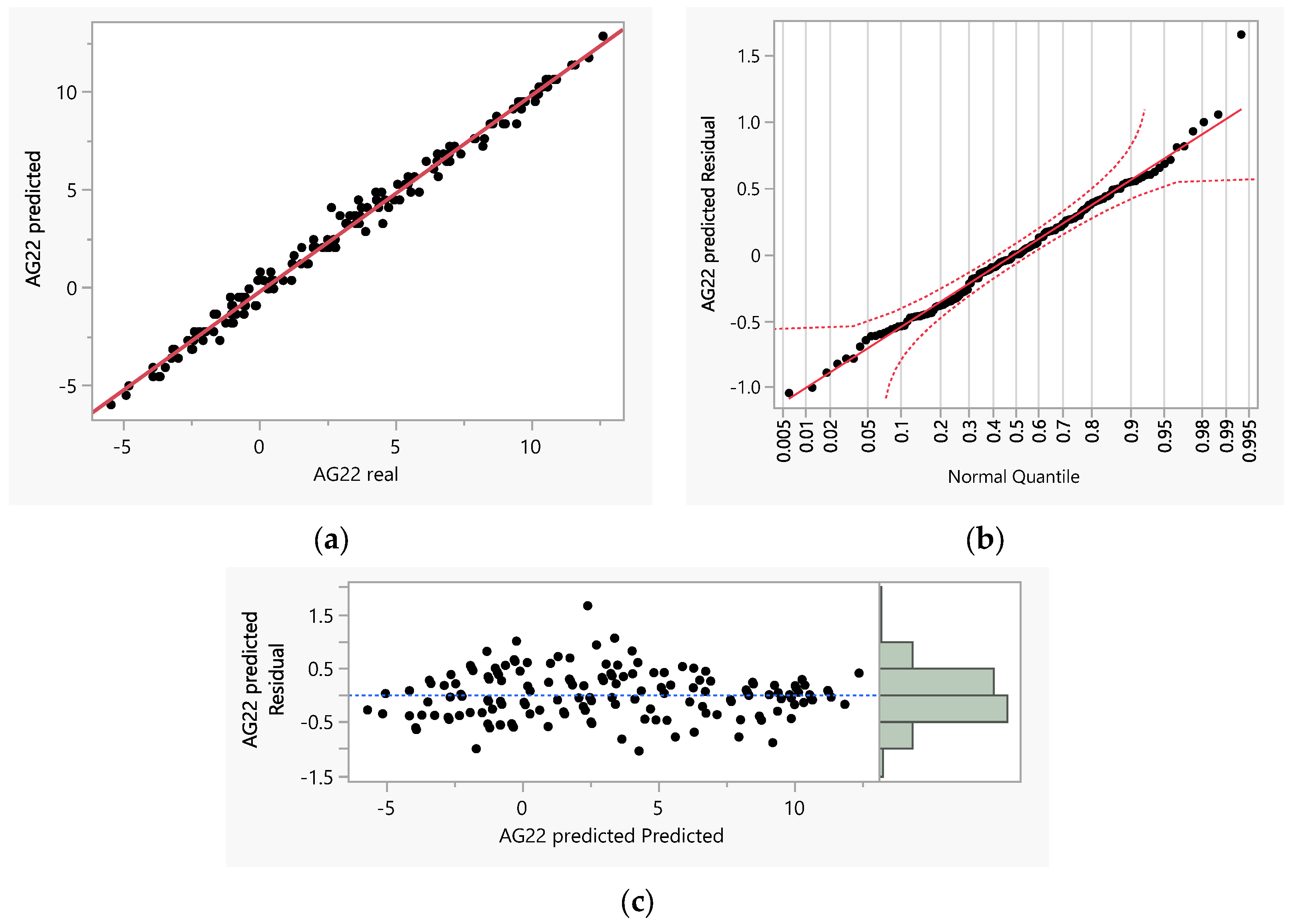
For validation and verification of the estimation model, independent data consisting of daily minimum temperatures from the year 2025 were utilized. The estimated results, when compared against actual measurement data, demonstrated correlations with R² values ranging from 0.97 to 0.99 and RMSE values from 0.34 to 0.58. To demonstrate the model’s appropriateness for the research area, illustrative diagrams are provided for the aforementioned study location, with Figure 2 offering visual validation of the model’s applicability.

3. Results and Conclusions

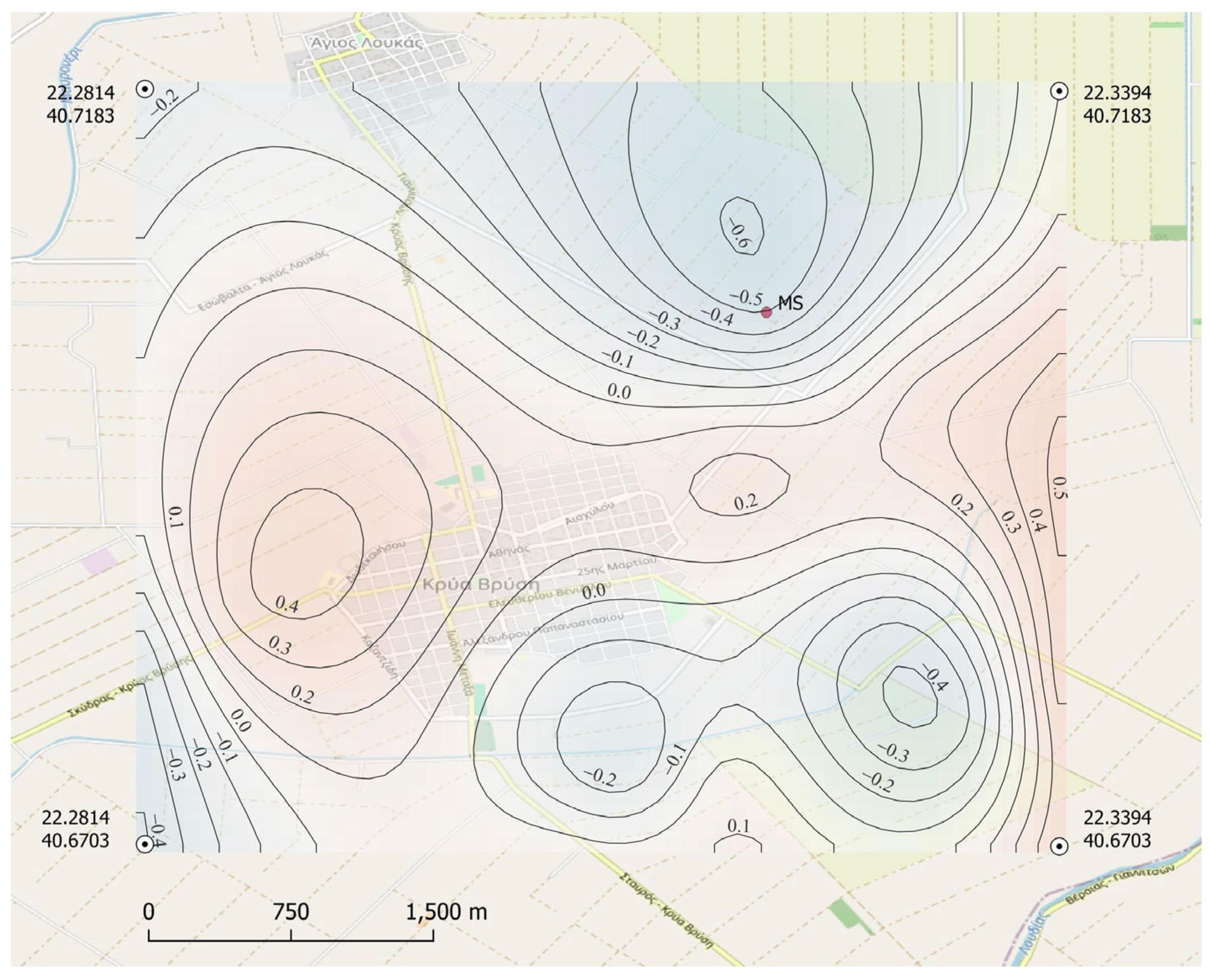
The developed methodology for real-time minimum temperature prediction in the fertile plain of Krya Vrysi, Pella, demonstrated exceptional performance and operational viability. The linear regression equations established between the reference telemetric meteorological station and the 12 autonomous temperature sensors with data loggers yielded remarkably high correlation coefficients, with R² values ranging from 0.98 to 0.99 and RMSE values between 0.35 and 0.60 °C during the model development phase. Residual analysis confirmed normal distribution patterns, validating the statistical robustness of the regression relationships. The spatial interpolation implementation using the Radial Basis Function method with thin plate splines kernel proved particularly effective for microclimatic data processing, providing smooth and accurate temperature distribution maps at 0.001° resolution (approximately 111 m), as shown in Figure 3.

Model validation using independent 2025 data confirmed the predictive reliability, with maintained high correlation coefficients (R² = 0.97–0.99) and low prediction errors (RMSE = 0.34–0.58 °C). These results demonstrate the model’s capacity to accurately estimate minimum temperatures across the study area using only reference station data, thereby providing agricultural producers with a practical tool for frost risk assessment and management. The methodology’s integration of statistical modelling with spatial interpolation techniques offers a significant advancement in operational agricultural meteorology, enabling targeted frost protection interventions and optimized resource allocation for crop protection strategies.

The proposed methodology establishes a robust framework for operational frost risk prediction in agricultural systems, demonstrating that high-accuracy minimum temperature estimation across complex terrain can be achieved through the integration of strategic meteorological station networks with advanced spatial interpolation techniques, thereby providing a scientifically validated tool for enhancing agricultural resilience against thermal stress events.

References

- Viggiano, Μ.; Busetto, L.; Cimini, D.; Di Paola, F.; Geraldi, E.; Ranghetti, L.; Ricciardelli, L.; Romano, F. A new spatial modeling and interpolation approach for high-resolution temperature maps combining reanalysis data and ground measurements. Agric. For. Meteorol. 2019, 276–277, 107590. [Google Scholar] [CrossRef]
- Rosillon, D.J.; Jago, A.; Huart, J.P.; Bogaert, P.; Jourée, M.; Dandrifosse, S.; Planchon, V. Near real-time spatial interpolation of hourly air temperature and humidity for agricultural decision support systems. Comput. Electron. Agric. 2024, 2023, 109093. [Google Scholar] [CrossRef]
- Chronopoulou-Sereli, A.; Flocas, A. Lessons of Agricultural Meteorology and Climatology; Ziti Publications: Thessaloniki, Greece, 2010; pp. 1–557. [Google Scholar]
- García-Martín, A.; Paniagua, L.L.; Moral, F.J.; Rebollo, F.J.; Rozas, M.A. Spatiotemporal Analysis of the Frost Regime in the Iberian Peninsula in the Context of Climate Change (1975–2018). Sustainability 2021, 13, 8491. [Google Scholar] [CrossRef]
- H.O.A.I. Activity Reports of H.O.A.I. for the Period of the Years 2014–2023; Department of Studies—Directorate of Studies and Applications and Education, Hellenic Organization of Agricultural Insurances (H.O.A.I.): Athens, Greece, 2024. [Google Scholar]
- Wratt, D.; Tait, A.; Giffiths, G.; Espic, P.; Jessen, M.; Keys, J.; Ladd, M.; Lew, D.; Lowther, W.; Mitchell, M.; et al. Climate for crops: Integrating climate data with information about soils and crop requirements to reduce risks in agricultural decision-making. Meteorol. Appl. 2006, 13, 305–315. [Google Scholar] [CrossRef]
- Webb, M.A.; Hall, A.; Kidd, D.; Minansy, B. Local-scale spatial modelling for interpolating climatic temperature variables to predict agricultural plant suitability. Theor. Appl. Climatol. 2016, 124, 1145–1165. [Google Scholar] [CrossRef]
- Luo, Z.; Wahba, G.; Johnson, D.R. Spatial–temporal analysis of temperature using smoothing spline ANOVA. J. Clim. 1998, 11, 19–28. [Google Scholar] [CrossRef]
- Vicente Serrano, S.M.; Sánchez, S.; Cuadrat, J.M. Comparative analysis of interpolation methods in the middle Ebro Valley (Spain): Application to annual precipitation and temperature. Clim. Change Res. Lett. 2003, 24, 161–180. [Google Scholar] [CrossRef]
- Im, H.; Rathouz, P.J.; Frederick, J.E. Space–time modeling of 20 years of daily air temperature in the Chicago metropolitan region. Environmetrics 2009, 20, 494–511. [Google Scholar] [CrossRef]
- Moeletsi, M.E.; Tongwane, M.I. Spatiotemporal Variation of Frost within Growing Periods. Adv. Meteorol. 2017, 2017, 5472869. [Google Scholar] [CrossRef]
- Wang, M.; He, G.; Zhang, Z.; Wang, G.; Zhang, Z.; Cao, X.; Wu, Z.; Liu, X. Comparison of spatial interpolation and regression analysis models for an estimation of monthly near surface air temperature in China. Remote Sens. 2017, 9, 1278. [Google Scholar] [CrossRef]
- Chen, T.; Xia, G.; Liu, T.; Du, S.; Zhou, H. Assessment of drought impact on main cereal crops using a standardized precipitation evapotranspiration index in Liaoning Province, China. Atmosphere 2015, 6, 1069–1096. [Google Scholar] [CrossRef]
- García-Martín, A.; Paniagua, L.L.; García, A.M.; Moral, F.J.; Rebollo, F.J. Spatial analysis of the relationship between olive leaf water content and physical-chemical soil properties in an olive orchard. Water 2015, 7, 1866–1886. [Google Scholar]
- Buhmann, M.D. Radial basis functions: Theory and implementations. Cambridge University Press: Cambridge, UK, 2003; pp. 1–259. [Google Scholar]
- Boer, G.J. Thin plate splines for mapping climate variables. Int. J. Appl. Earth Obs. Geoinf. 2001, 3, 146–154. [Google Scholar] [CrossRef]