Proceeding Paper

Effect of Nitrogen Oxide Concentration Levels and Meteorological Variables on Ozone (O3) Formation in the Petrochemical Industry Area in the Monterrey Metropolitan, Mexico †

by
Jailene Marlen Jaramillo-Perez
,
Bárbara A. Macías-Hernández
,
Edgar Tello-Leal
* and
René Ventura-Houle
Faculty of Engineering and Science, Autonomous University of Tamaulipas, Victoria 87000, Mexico
*
Author to whom correspondence should be addressed.
Presented at the 7th International Electronic Conference on Atmospheric Sciences (ECAS-7), 4–6 June 2025; Available online: https://sciforum.net/event/ECAS2025.
Environ. Earth Sci. Proc. 2025, 34(1), 3; https://doi.org/10.3390/eesp2025034003
Published: 8 August 2025

Abstract

The petrochemical industry emits large amounts of nitrogen oxides (NOx). It is the second source of volatile organic compounds (VOCs), which, through photochemical reactions, can form tropospheric ozone (O3) and, together with geographic and meteorological conditions, influence the spatial and temporal behavior of pollution. The objective of this study is to assess the influence of air pollutants NOx, NO2, and NO, as well as meteorological factors on O3 concentration levels in the city of Cadereyta, Nuevo Leon, which is characterized by its petrochemical industry as part of the metropolitan area of Monterrey, Mexico. The data were analyzed using the Spearman’s correlation coefficient, identifying a weak-to-moderate negative association between NOx and NO2 with O3 in the spring season and a null relationship in the summer. However, the autumn and winter seasons observed a moderate to strong negative relationship. Subsequently, a multiple linear regression analysis determined the influence of air pollutants NOx, NO2, and NO, as well as meteorological factors on O3 concentration levels. In this sense, when the concentration levels of NOx and NO2 decrease, the concentration of O3 will increase proportionally according to the season of the year. The prediction model obtains a coefficient of determination (R2) of 0.60 and a root-mean-square error (RMSE) value of 0.0096 ppm. In the prediction model, all variables presented a significant effect on the interpretation of the dependent variable. The independent variables that provided the most significant variation in the concentration levels of O3 were NOx and NO2.

1. Introduction

In several cities, the petrochemical industry is located within urban areas, becoming the primary source of air pollutants, followed by emissions from heavy goods transport and private vehicles. These sources cause higher levels of volatile organic compounds (VOCs) and nitrogen oxides (NOx), which, through photochemical reactions, contribute to the increase in tropospheric ozone (O3) concentrations. This pollutant frequently exceeds the limits established by both national and international regulations, representing a risk to human health and ecosystems [1,2]. The most common emissions in the petrochemical industry are VOCs [3], primarily at crude oil extraction and refining sites [4], where alkanes, alkenes, and aromatics are particularly notable, as they are considered to have the highest ozone formation potential [5,6,7].
The relationship between O3 and its precursors has been studied to develop mitigation or reduction strategies. However, O3 concentrations are influenced by the abundance of their precursors and by climatic variations, which allow them to exhibit hourly and seasonal patterns [8]. These patterns generally do not follow a linear trend. Although there is an association between O3 and meteorological variables [9], the levels of correlation vary across different study areas [10]. Some of the most examined factors are temperature and relative humidity, with an increase in O3 concentration reported when high temperatures, low relative humidity, and light winds occur. Additionally, the effects of air pollutant transport and solar radiation have been considered [11,12,13]. In [14], the authors observed that O3 levels decrease during land storms. Furthermore, it has been observed that under conditions of precipitation and high wind speeds, O3 concentration levels decrease, aiding dispersion [15].
On the other hand, it has been reported that meteorological phenomena cause climate changes that intensify O3 pollution [16]. The presence of high atmospheric pressure systems (anticyclones) is characterized by low cloud cover, increased solar radiation, and an increase in photochemical reactions that favor the accumulation O3 [17]. In this context, temperature is one of the primary factors that generate extreme air pollution events, often associated with heatwaves and extreme droughts [18]. Conversely, increased relative humidity is associated with decreased O3 concentrations [9], as it leads to greater cloud formation, reducing photochemical reactions and solar radiation levels [19].
Therefore, meteorology can influence O3 variability in both space and time, from daily patterns to long-term trends [13]. Hence, the objective of this paper is to assess the influence of air pollutants NOx, NO2, and NO, along with meteorological parameters, on O3 concentration levels in the city of Cadereyta, Nuevo León, México. This city is renowned for its petrochemical industry and is situated within the industrial area of the Monterrey metropolitan region in México.

2. Materials and Methods

2.1. Area of Study

Air pollution and meteorological data were collected in the city of Cadereyta, Nuevo León, located in northeastern México. This city is part of the Monterrey metropolitan area, Mexico. It is characterized by a semi-warm, sub-humid climate with limited rainfall throughout the year, and temperatures range from 20 to 24 °C. However, during summer, temperatures can exceed 40 °C, and in winter, they can drop below 0 °C. The prevailing winds in the area blow from the southeast to the northeast, with mountainous terrain that promotes the accumulation of pollutants at ground level [20]. The main economic activities include industry, oil extraction, and refining, where products such as gasoline, diesel, propylene, and sulfur are produced.

2.2. Data Collection

The dataset was collected through the air quality monitoring station in the city of Cadereyta, which is part of the Comprehensive Environmental Monitoring System (SIMA) of the Nuevo León state government. We retrieved the data using queries in the open data repository of the National Air Quality Information System, a government initiative in Mexico. The monitoring station is located in the northeast of the municipality and covers a 4 km2 radius, near a petroleum refining plant with a large production capacity. The station can record the concentration of air pollutants and meteorological factors, reporting hourly average values throughout the year. The dataset includes hourly mean values of the variables such as O3, NOx, NO, NO2, temperature (T), relative humidity (RH), barometric pressure (BP), wind speed (WS), and wind direction (WD), covering the period from 22 September 2022 to 21 September 2023, with measurements recorded from 00:00 to 23:00 each day.

2.3. Data Analysis

The data were analyzed using RStudio software version 4.3.0. Spearman’s correlation coefficient analysis was applied to evaluate the relationship between meteorological variables and pollutant concentration levels. The correlation was described in terms of the parameters, considering the p-value. Subsequently, to determine the influence of NOx, NO, NO2, and the meteorological parameters (T, RH, BP, WS, and WD) on O3 formation, a multiple linear regression (MLR) model was designed. The variable values were normalized using the minimum–maximum method. The most relevant predictor variables were then identified and selected for the regression model, implementing the stepwise method. The performance of the multiple linear regression model was measured using the coefficient of determination (R2) and root-mean-square error (RMSE), which assess the accuracy of the prediction model. The RMSE metric represents the error between the actual values and the values predicted by the model. Values range from 0 to 1, and acceptable error values are those close to 0. R2 indicates the percentage of variation between the measured values and the model’s predictions. Values range from 0 to 1, with values close to 1 indicating that the values are compatible with each other.

3. Results and Discussion

3.1. Correlation Analysis

The Spearman’s correlation matrix shows that the coefficients between air pollutants tend to behave similarly during autumn and winter. There is a moderate negative association between O3 and NOx variables, with values of −0.52 in autumn and −0.55 in winter (see Figure 1). Recent studies indicate that higher O3 concentrations are often correlated with lower NOx levels due to photolysis of this precursor [21], which may explain the association identified between these air pollutants. Next, a moderate negative relationship was found between O3 and NO2, with coefficients of −0.46 and −0.55 (p-value < 0.05), consistent with Li et al. [22], who reported correlations of −0.21 in autumn and 0.18 in winter. Furthermore, a moderate negative correlation was observed between O3 and NO, with a value of −0.57 and −0.53 for both seasons. A very strong positive association was observed between NO2 and NOx (0.91 in winter), and a strong positive relation between NO and NOx (0.77 in autumn and 0.85 in winter). The ranges for NO2 and NO correlations were 0.69 and 0.90 for autumn and winter, respectively. Conversely, weak-to-negligible negative correlations were identified between the temperature variable and NO, NOx, and NO2, as well as negligible correlations with RH.
On the other hand, the association of ozone with NOx, NO2, and NO emissions during the spring was weak, with values of −0.39, −0.39, and −0.38, respectively. In summer, values lower than −0.1 were recorded (see Figure 1). It is essential to consider that the weak or nonexistent correlations between O3 and its precursors may be due to high temperatures, which promote the transformation cycles of these air pollutants, as well as the continuous formation of NOx or its depletion to produce O3 [23]. Likewise, the relationship between O3 and meteorological variables during autumn and winter exhibited a moderately positive association with temperature, with coefficients of 0.51 and 0.42, respectively. This moderate relationship strengthened during spring and summer, with values reaching 0.48 and 0.67, respectively. Consequently, a similar influence of temperature is observed across all four seasons, with a notable increase in summer, indicating a moderately high correlation (see Figure 1).
In contrast, a negative relationship was observed between O3 and relative humidity, with values of −0.57 and −0.56 for autumn and winter, respectively. During spring, the values were −0.58 and −0.67 for summer (see Figure 1); this pattern aligns with reports by [24], which found that relative humidity negatively influences O3 levels. The correlations between O3 and WS were positive and moderate during spring, autumn, and winter. This factor has been shown to impact O3 concentrations due to changes in horizontal transport and vertical mixing [25]. Regarding WD, a weak negative association was noted in autumn (−0.27) and winter (−0.33). Therefore, it can be assumed that both the concentration of air pollutants and the relationship identified between them are strongly associated with the variability in temperature, relative humidity, and prevailing wind speed during autumn and winter, which promote the accumulation of surface O3 [21].

3.2. O3 Prediction Models

The most effective predictor variables were chosen using the stepwise method by season. Therefore, for the winter model, the variables NO2, NOx, WD, RH, BP, T, and WS were included. In the autumn model, the predictor variables NO2, NO, NOx, WD, RH, BP, T, and WS were selected. For the spring model, only NO2, NOx, RH, BP, and T were used; and in the summer model, NO2, NO, NOx, WD, RH, T, and WS were included. Different combinations of predictor variables were used across the four multiple linear regression models. Regression analysis identified that the best model for estimating O3 concentration levels was derived from the winter season dataset. In this model, the equation that includes the NO variable obtains an R2 value of 0.6055 (similar to the model that excluded the NO variable) but has a higher residual standard error (RSE) of 0.009583. This value indicates the model’s accuracy; the lower the RSE, the better the model fits the data. In the model without the NO variable, the RSE was 0.009581. In this sense, the inclusion of some variables can introduce noise or redundancy if there is multicollinearity or weak correlations between them, as is present in these models.
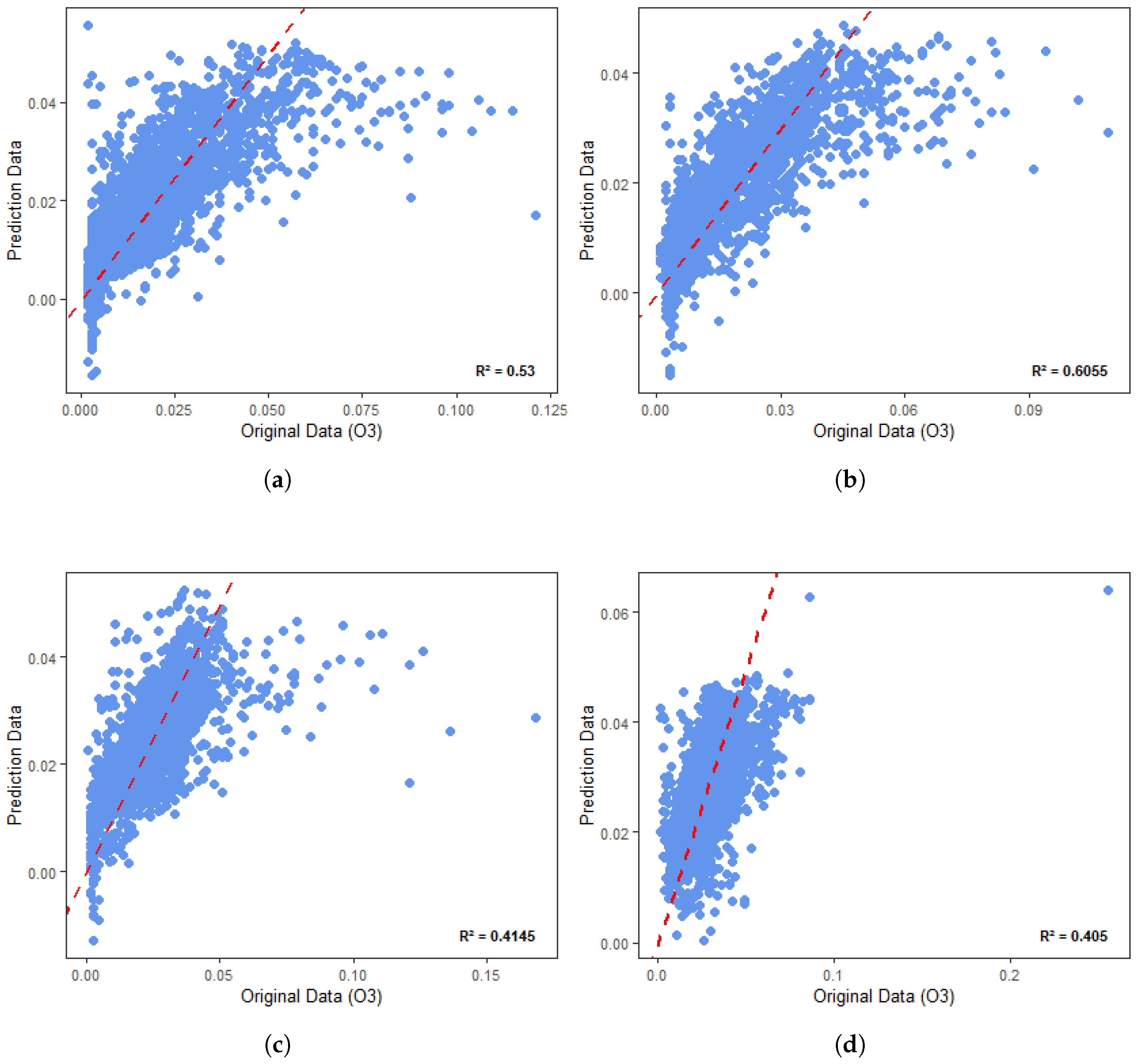
The winter model can predict O3 concentration values in the spring, summer, and winter seasons with a RMSE of 0.0096 ppm. The linear trend with the best fitness among the scattered R2 points for the model with the winter data was 0.60 (see Table 1). For the autumn, the prediction model yielded an R2 of 0.53 and a RMSE of 0.0115 ppm, while in the spring, it achieved an R2 of 0.41 and a RMSE of 0.0111 ppm. Finally, the summer prediction model obtained an R2 of 0.40 and a RMSE of 0.0111. The values in the metrics show that the prediction model explains a significant percentage of O3 variability and exhibits better predictive accuracy.
From the analysis, it was identified that the intercept coefficient in the winter model was −0.1817; for the NO2 variable, the coefficient was −0.6349, and for NOx, −0.024335 (see Equation (1)). This indicates that when NO2 and NOx concentrations decrease, O3 levels will increase by −0.6349 and −0.024335 ppm, respectively. In contrast, when NO2 and NOx concentrations increase, O3 levels will decrease by −0.6349 and −0.024335 ppm, respectively. Hence, during the solar absorption of NO2, it is transformed into NO and atomic oxygen. In this process, atomic oxygen binds to an oxygen molecule (O2) to form O3. Under normal conditions, O3 and NO react to produce oxygen and NO2, completing the NO2 cycle. The above can be linked to the value of the NO2 coefficient in Equation (1). Additionally, during the winter season, lower solar radiation reduces photochemical reactions that produce O3, resulting in higher NOx concentrations and lower O3 levels compared to spring and summer. In autumn, lower solar radiation also suppresses photochemical reactions. However, O3 levels may increase due to accumulation caused by low dispersion from low wind speeds, coupled with pollutant transport, as winds predominantly blow from the southeast (the location of the refinery) to the northeast (the location of the monitoring station and urban area).
On the other hand, temperature has a positive coefficient of 0.0006412, relative humidity has a negative coefficient of −0.0003127, barometric pressure has a coefficient of 0.0003004, and wind direction and speed have coefficients of −0.000007986 and 0.0005662, respectively. According to R2, the model explains 60.55% of the variability in O3 concentration based on its independent variables, with a RMSE of 0.0096. Therefore, we concluded that the variables NOx, NO2, T, and RH are the most significant in determining O3 levels during winter, indicating that interactions among primary pollutants strongly influence ozone. Equations (2)–(4) show the regression coefficients and independent variables for the dependent variable Y i in the models predicting O3 concentration for autumn, spring, and summer, respectively.
Y i = 0.1817 0.6349 N O 2 0.02433 N O x 0.000007986 W D 0.0003127 R H + 0.0003004 B P + 0.0006412 T 0.0005662 W S
Y i = 0.2482 0.8549 N O 2 0.4877 N O + 0.3704 N O x 0.00001127 W D 0.0003855 R H + 0.0003945 B P + 0.0007054 T + 0.0008025 W S
Y i = 0.2065 0.5110 N O 2 0.1988 N O x 0.0003289 R H + 0.0003402 B P + 0.0004571 T
Y i = 0.04190 0.4412 N O 2 0.8011 N O + 0.4885 N O x + 0.00001360 W D 0.0004081 R H + 0.0005116 T 0.003002 W S
Figure 2 illustrates the relationship between observed and predicted data (O3) concentrations using a multiple linear regression model for the four seasons. The winter model (see Figure 2b) exhibits better performance (R2 = 0.6054, RMSE = 0.0096), but it presents an overestimation in O3 concentrations above 0.04 ppm. Conversely, in the range of values below 0.015 ppm, the model presents an underestimation, which is reflected in predictions that are lower than the observed data. The model explains 60.55% of the variability in the data, representing a moderate and acceptable fit. Following this, the model for the autumn season presents a defined pattern based on the actual values and significant variability in the data (see Figure 2a). Furthermore, an overestimation is observed for concentrations above 0.4 ppm. The spring model exhibits a wide dispersion in predicted values, with limited performance (R2 = 0.4145 and RMSE = 0.0111). Moreover, the most consistent predicted values are found in concentrations between 0.037 and 0.045 ppm, identifying that accuracy decreases at extremely low and high values (see Figure 2c). Finally, the summer model presents R2 = 0.4050 and RMSE = 0.0111, with the lowest metrics compared to the models corresponding to the other seasons; however, the data present an acceptable fit (see Figure 2d).
The poor performance could be associated with complex relationships between the predictor variables and O3. These models indicate that the meteorological conditions prevailing during these seasons play a significant role in ozone formation, resulting in greater variability, which the models fail to capture. However, although the relationship between O3 and its precursors is not necessarily linear, its behavior is influenced by a complex interaction with variables such as solar radiation, temperature, relative humidity, and wind speed, as well as by geographical conditions that can favor the accumulation of pollutants due to weak atmospheric circulation, which is consistent with the findings of [26,27,28]. Moreover, although the models generated in this study allow for the identification of direct relationships between atmospheric variables and O3 concentration, their predictive capacity is limited by the multicollinearity between variables and the nonlinear complexity of the chemical reactions involved, especially during warm seasons, when dynamic meteorological patterns and complex secondary formation processes predominate.
Therefore, the limitation of these models can be used to define or design nonlinear models when the same conditions are present in the variables used in our study. It is also possible to incorporate cyclical and lag variables to improve the performance and accuracy of the regression model. Furthermore, machine learning models or logarithmic transformations could be used to extract greater linearity from the variables.

3.3. Residuals

The histograms of the residuals from each seasonal model display distributions with symmetric magnitudes close to zero, indicating that the residuals exhibit normal behavior, characterized by relatively constant dispersion (see the plots at the top of Figure 3). This suggests that the homoscedasticity assumption is met in most models. Additionally, when comparing the residuals with the fitted values, it is observed that the autumn and winter models exhibit more homogeneous and horizontal dispersion (see Figure 3e,f). Furthermore, the spring and summer models exhibit curvature patterns, indicating that not all predictor variables are contributing significantly to the model (see Figure 3g,h). That is, other variables exert a greater influence, as indicated by the coefficient obtained in the regression model. The equations derived from the model revealed that the variables NOx, T, WS, WD, and BP significantly influenced surface O3 production.

4. Conclusions

This study analyzed the concentration levels of O3, NO, NOx, NO2, and meteorological factors in Cadereyta, Mexico. Correlation analysis revealed a strong positive relationship between NO, NOx, and NO2, as well as a negative association between O3 and its precursors. Additionally, it demonstrated a strong positive correlation with temperature and a negative correlation with relative humidity. Similar patterns were observed in both autumn and winter. Finally, multiple linear regression analysis identified that the best model to estimate O3 concentration levels is derived from the winter season dataset, which can predict with an R2 of 0.6055 and a RMSE of 0.0096, representing acceptable precision and performance, highlighting that O3 concentrations are significantly correlated with temperature, relative humidity, NOx, and NO2, since these variables proportionally influence O3 formation in the study area.

Author Contributions

Conceptualization, B.A.M.-H. and E.T.-L.; methodology, J.M.J.-P., B.A.M.-H. and E.T.-L.; software, J.M.J.-P. and E.T.-L.; validation, J.M.J.-P., B.A.M.-H. and E.T.-L.; formal analysis, J.M.J.-P., B.A.M.-H., E.T.-L. and R.V.-H.; investigation, J.M.J.-P., B.A.M.-H., E.T.-L. and R.V.-H.; resources, E.T.-L.; data curation, J.M.J.-P. and E.T.-L.; writing—original draft preparation, J.M.J.-P., B.A.M.-H. and E.T.-L.; writing—review and editing, J.M.J.-P., B.A.M.-H. and E.T.-L.; visualization, J.M.J.-P. and E.T.-L.; supervision, B.A.M.-H.; project administration, E.T.-L.; funding acquisition, E.T.-L. All authors have read and agreed to the published version of the manuscript.

Funding

The Autonomous University of Tamaulipas partially funded this research. Additionally, the study received partial funding from the Secretariat of Science, Humanities, Technology, and Innovation (SECIHTI) through grant 1239803 (Jailene Marlen Jaramillo-Perez).

Institutional Review Board Statement

Not applicable.

Informed Consent Statement

Not applicable.

Data Availability Statement

The original data presented in the study are openly available in https://sinaica.inecc.gob.mx/ (accessed on 17 March 2025).

Conflicts of Interest

The authors declare no conflicts of interest.

References

  1. Guo, W.; Yang, Y.; Chen, Q.; Zhu, Y.; Zhang, Y.; Zhang, Y.; Liu, Y.; Li, G.; Sun, W.; She, J. Chemical reactivity of volatile organic compounds and their effects on ozone formation in a petrochemical industrial area of Lanzhou, Western China. Sci. Total Environ. 2022, 839, 155901. [Google Scholar] [CrossRef]
  2. Pinthong, N.; Thepanondh, S.; Kultan, V.; Keawboonchu, J. Characteristics and Impact of VOCs on Ozone Formation Potential in a Petrochemical Industrial Area, Thailand. Atmosphere 2022, 13, 732. [Google Scholar] [CrossRef]
  3. Liang, X.; Sun, X.; Xu, J.; Ye, D. Improved emissions inventory and VOCs speciation for industrial OFP estimation in China. Sci. Total Environ. 2020, 745, 140838. [Google Scholar] [CrossRef] [PubMed]
  4. Tang, J.; Shen, H.; Li, H.; Ji, Y.; Zhong, X.; Zhao, M.; Liu, Y.; Guo, M.; Shang, F.; Xue, L. Significant contributions of the petroleum industry to volatile organic compounds and ozone pollution: Insights from year-long observations in the Yellow River Delta. Atmos. Ocean. Sci. Lett. 2024, 17, 100523. [Google Scholar] [CrossRef]
  5. Yang, Y.; Meng, X.; Chen, Q.; Xue, Q.; Wang, L.; Sun, J.; Guo, W.; Tao, H.; Yang, L.; Chen, F. Characteristics of volatile organic compounds under different operating conditions in a petrochemical industrial zone and their effects on ozone formation. Environ. Pollut. 2024, 363, 125254. [Google Scholar] [CrossRef] [PubMed]
  6. Lee, G.; Kim, S.J.; Choi, S.D. Influence of industrial emissions on volatile organic compound levels and secondary formation of organic aerosol and ozone in a multi-industrial city during the warm season. Atmos. Environ. 2025, 343, 120983. [Google Scholar] [CrossRef]
  7. Ding, Z.; Li, Y.; Fu, Q.; Tian, M.; Wang, F.; Wang, Y.; Huang, K. Volatile organic compounds in a typical petrochemical production area in Shanghai, China: Source profiles, human health and environmental impacts. Environ. Pollut. 2025, 372, 126074. [Google Scholar] [CrossRef]
  8. Tang, Y.; Wang, Y.; Chen, X.; Liang, J.; Li, S.; Chen, G.; Chen, Z.; Tang, B.; Zhu, J.; Li, X. Diurnal emission variation of ozone precursors: Impacts on ozone formation during Sep. 2019. Sci. Total Environ. 2024, 929, 172591. [Google Scholar] [CrossRef] [PubMed]
  9. Lin, C.; Lau, A.K.; Fung, J.C.; Song, Y.; Li, Y.; Tao, M.; Lu, X.; Ma, J.; Lao, X.Q. Removing the effects of meteorological factors on changes in nitrogen dioxide and ozone concentrations in China from 2013 to 2020. Sci. Total Environ. 2021, 793, 148575. [Google Scholar] [CrossRef]
  10. Ji, X.; Hong, Y.; Lin, Y.; Xu, K.; Chen, G.; Liu, T.; Xu, L.; Li, M.; Fan, X.; Wang, H.; et al. Impacts of Synoptic Patterns and Meteorological Factors on Distribution Trends of Ozone in Southeast China During 2015–2020. J. Geophys. Res. Atmos. 2023, 128, e2022JD037961. [Google Scholar] [CrossRef]
  11. Zhang, C.; Luo, S.; Zhao, W.; Wang, Y.; Zhang, Q.; Qu, C.; Liu, X.; Wen, X. Impacts of Meteorological Factors, VOCs Emissions and Inter-Regional Transport on Summer Ozone Pollution in Yuncheng. Atmosphere 2021, 12, 1661. [Google Scholar] [CrossRef]
  12. Hu, C.; Kang, P.; Jaffe, D.A.; Li, C.; Zhang, X.; Wu, K.; Zhou, M. Understanding the impact of meteorology on ozone in 334 cities of China. Atmos. Environ. 2021, 248, 118221. [Google Scholar] [CrossRef]
  13. Borhani, F.; Shafiepour Motlagh, M.; Stohl, A.; Rashidi, Y.; Ehsani, A.H. Tropospheric Ozone in Tehran, Iran, during the last 20 years. Environ. Geochem. Health 2022, 44, 3615–3637. [Google Scholar] [CrossRef]
  14. Wang, L.; Zhao, Y.; Shi, J.; Ma, J.; Liu, X.; Han, D.; Gao, H.; Huang, T. Predicting ozone formation in petrochemical industrialized Lanzhou city by interpretable ensemble machine learning. Environ. Pollut. 2023, 318, 120798. [Google Scholar] [CrossRef] [PubMed]
  15. Chen, Z.; Li, R.; Chen, D.; Zhuang, Y.; Gao, B.; Yang, L.; Li, M. Understanding the causal influence of major meteorological factors on ground ozone concentrations across China. J. Clean. Prod. 2020, 242, 118498. [Google Scholar] [CrossRef]
  16. Kusumaningtyas, S.D.A.; Tonokura, K.; Muharsyah, R.; Gunawan, D.; Sopaheluwakan, A.; Iriana, W.; Lestari, P.; Permadi, D.A.; Rahmawati, R.; Samputra, N.A.R. Comprehensive analysis of long-term trends, meteorological influences, and ozone formation sensitivity in the Jakarta Greater Area. Sci. Rep. 2024, 14, 9605. [Google Scholar] [CrossRef]
  17. Nguyen, D.H.; Lin, C.; Vu, C.T.; Cheruiyot, N.K.; Nguyen, M.K.; Le, T.H.; Lukkhasorn, W.; Vo, T.D.H.; Bui, X.T. Tropospheric ozone and NOx: A review of worldwide variation and meteorological influences. Environ. Technol. Innov. 2022, 28, 102809. [Google Scholar] [CrossRef]
  18. Lin, X.; Yuan, Z.; Yang, L.; Luo, H.; Li, W. Impact of Extreme Meteorological Events on Ozone in the Pearl River Delta, China. Aerosol Air Qual. Res. 2019, 19, 1307–1324. [Google Scholar] [CrossRef]
  19. Han, H.; Liu, J.; Shu, L.; Wang, T.; Yuan, H. Local and synoptic meteorological influences on daily variability in summertime surface ozone in eastern China. Atmos. Chem. Phys. 2020, 20, 203–222. [Google Scholar] [CrossRef]
  20. Mancilla, Y.; Paniagua, I.H.; Mendoza, A. Spatial differences in ambient coarse and fine particles in the Monterrey metropolitan area, Mexico: Implications for source contribution. J. Air Waste Manag. Assoc. 2019, 69, 548–564. [Google Scholar] [CrossRef]
  21. Allu, S.K.; Srinivasan, S.; Maddala, R.K.; Reddy, A.; Anupoju, G.R. Seasonal ground level ozone prediction using multiple linear regression (MLR) model. Model. Earth Syst. Environ. 2020, 6, 1981–1989. [Google Scholar] [CrossRef]
  22. Li, X.; Abdullah, L.C.; Sobri, S.; Md Said, M.S.; Hussain, S.A.; Aun, T.P.; Hu, J. Long-Term Air Pollution Characteristics and Multi-scale Meteorological Factor Variability Analysis of Mega-mountain Cities in the Chengdu-Chongqing Economic Circle. Water Air Soil Pollut. 2023, 234, 328. [Google Scholar] [CrossRef]
  23. Baidrulhisham, S.E.; Noor, N.M.; Hassan, Z.; Sandu, A.V.; Vizureanu, P.; Ul-Saufie, A.Z.; Zainol, M.R.R.M.A.; Kadir, A.A.; Deák, G. Effects of Weather and Anthropogenic Precursors on Ground-Level Ozone Concentrations in Malaysian Cities. Atmosphere 2022, 13, 1780. [Google Scholar] [CrossRef]
  24. Paraschiv, S.; Barbuta-Misu, N.; Paraschiv, S.L. Influence of NO2, NO and meteorological conditions on the tropospheric O3 concentration at an industrial station. Energy Rep. 2020, 6, 231–236. [Google Scholar] [CrossRef]
  25. Fang, C.; Wang, L.; Wang, J. Analysis of the Spatial–Temporal Variation of the Surface Ozone Concentration and Its Associated Meteorological Factors in Changchun. Environments 2019, 6, 46. [Google Scholar] [CrossRef]
  26. Ren, S.; Ji, X.; Zhang, X.; Huang, M.; Li, H.; Wang, H. Characteristics and Meteorological Effects of Ozone Pollution in Spring Season at Coastal City, Southeast China. Atmosphere 2022, 13, 2000. [Google Scholar] [CrossRef]
  27. Mao, J.; Wang, L.; Lu, C.; Liu, J.; Li, M.; Tang, G.; Ji, D.; Zhang, N.; Wang, Y. Meteorological mechanism for a large-scale persistent severe ozone pollution event over eastern China in 2017. J. Environ. Sci. 2020, 92, 187–199. [Google Scholar] [CrossRef]
  28. Petrus, M.; Popa, C.; Bratu, A.M. Temporal Variations in Urban Air Pollution during a 2021 Field Campaign: A Case Study of Ethylene, Benzene, Toluene, and Ozone Levels in Southern Romania. Sustainability 2024, 16, 3219. [Google Scholar] [CrossRef]
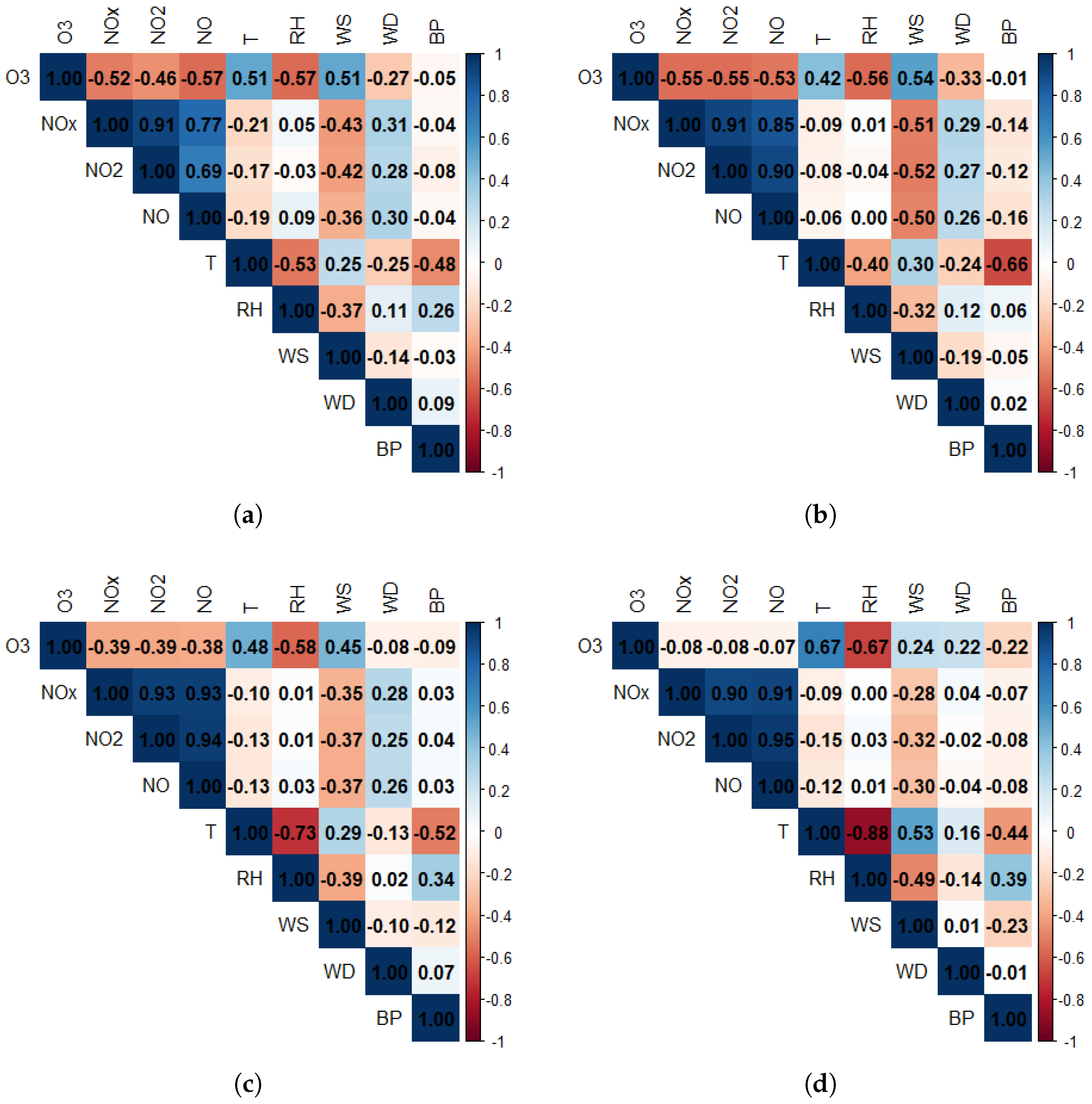
Figure 1. Correlation matrixof variables of study: (a) autumn, (b) winter, (c) spring, and (d) summer.
Eesp 34 00003 g001
Figure 2. Scatter plot of original (actual) data versus predicted data of O3 concentration (ppm) for (a) autumn, (b) winter, (c) spring, and (d) summer models. The blue dots represent the data points, and the red line represents the best-fit line determined by the linear regression model.
Eesp 34 00003 g002
Figure 3. Visualizing residual distribution from regression models.: (a) autumn, (b) winter, (c) spring, and (d) summer. The residuals vs. fitted plots: (e) autumn, (f) winter, (g) spring, and (h) summer.
Eesp 34 00003 g003
Table 1. Values obtained by each model for the performance metrics.
Season R 2 RMSE
Autumn0.530.0115
Winter0.600.0096
Spring0.410.0111
Summer0.400.0111
Disclaimer/Publisher’s Note: The statements, opinions and data contained in all publications are solely those of the individual author(s) and contributor(s) and not of MDPI and/or the editor(s). MDPI and/or the editor(s) disclaim responsibility for any injury to people or property resulting from any ideas, methods, instructions or products referred to in the content.