
Numerical Analysis of Debris Impact Forces and Its Environmental Repercussions Using Smoothed Particle Hydrodynamics †

 ,
,  ,
,
Abstract
1. Introduction
2. Smoothed Particle Hydrodynamics (SPH) Formulation
3. Methodology
3.1. Validation of the Developed SPH Model
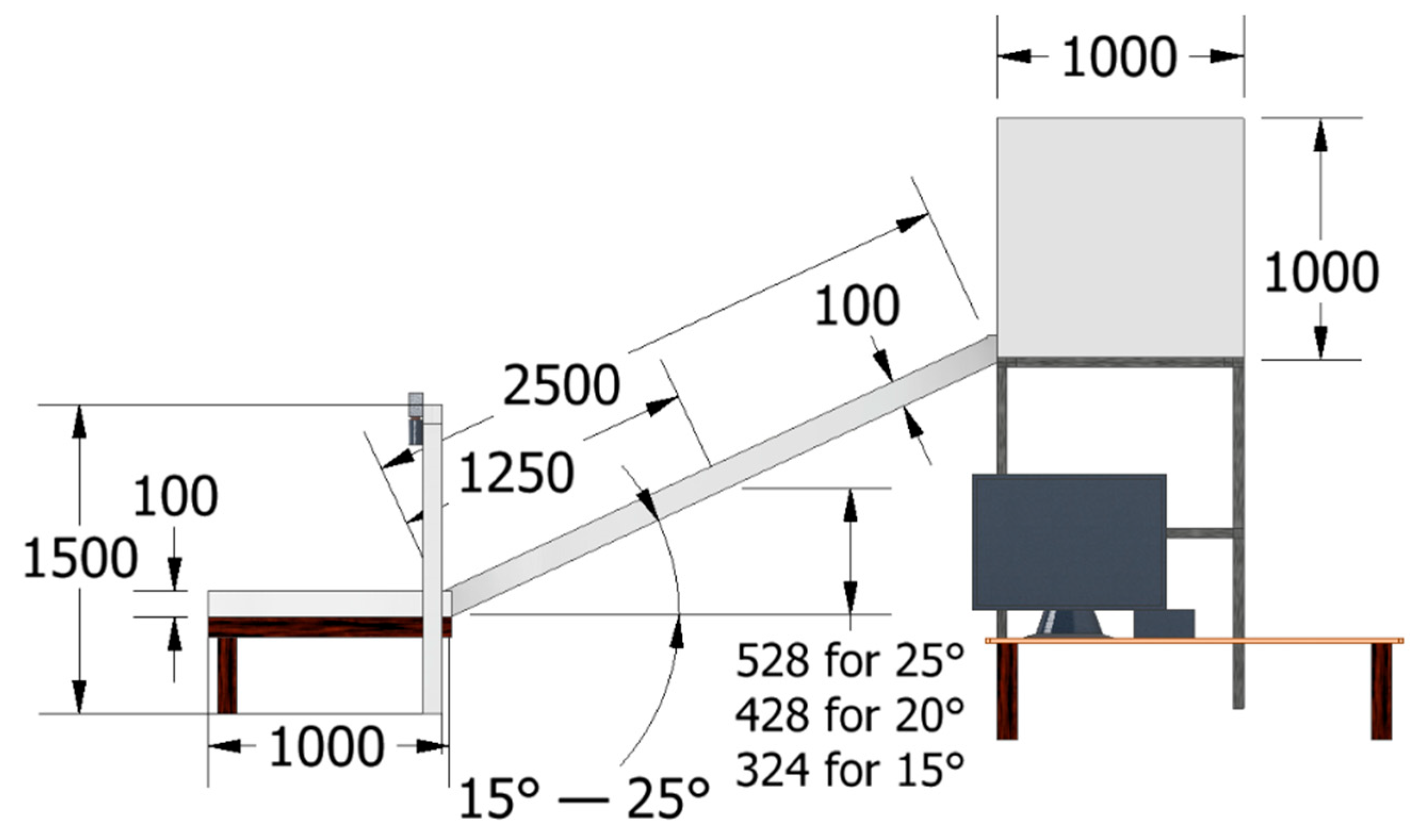
3.2. Experimental Setup for Debris Flow Model Test for Validation
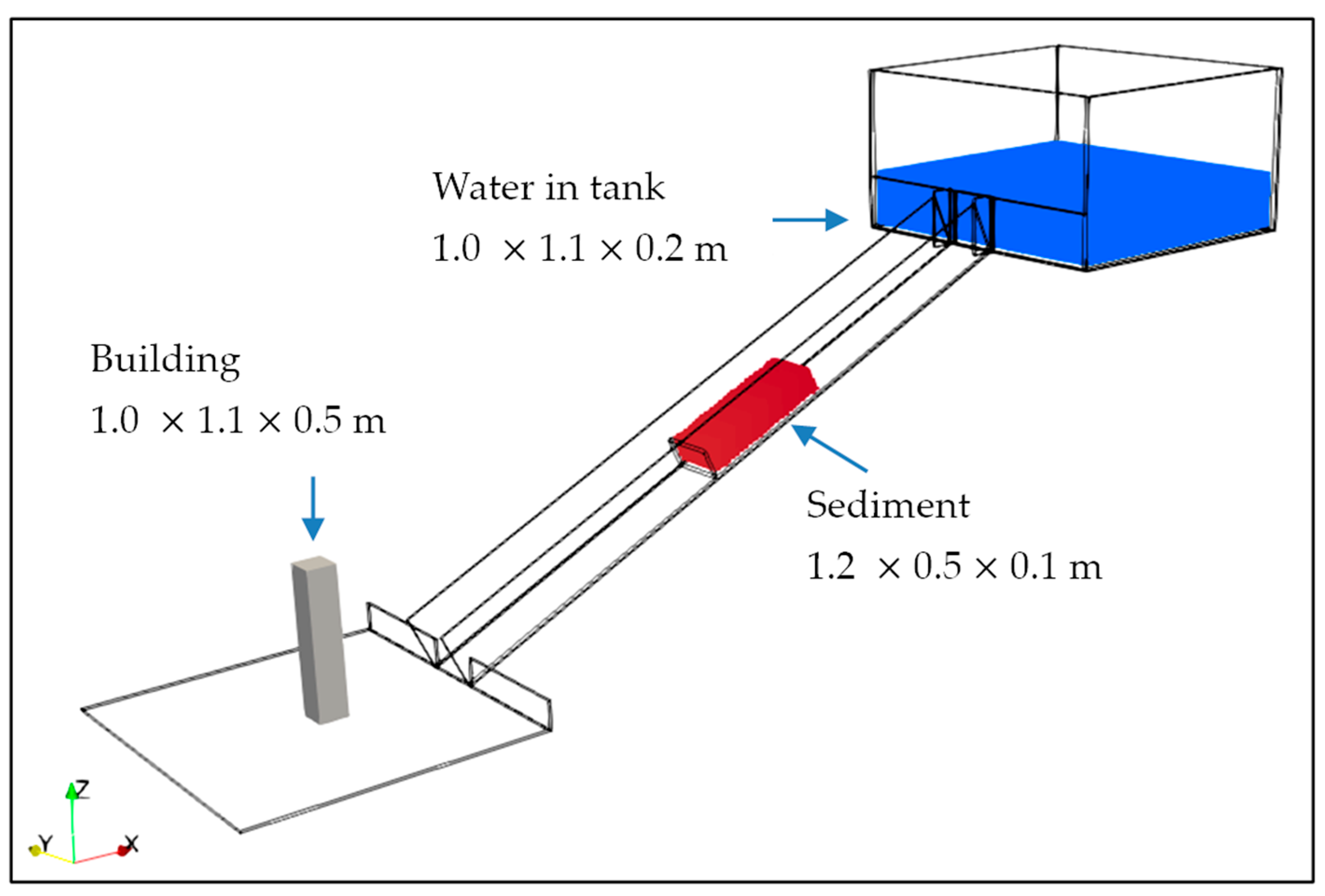
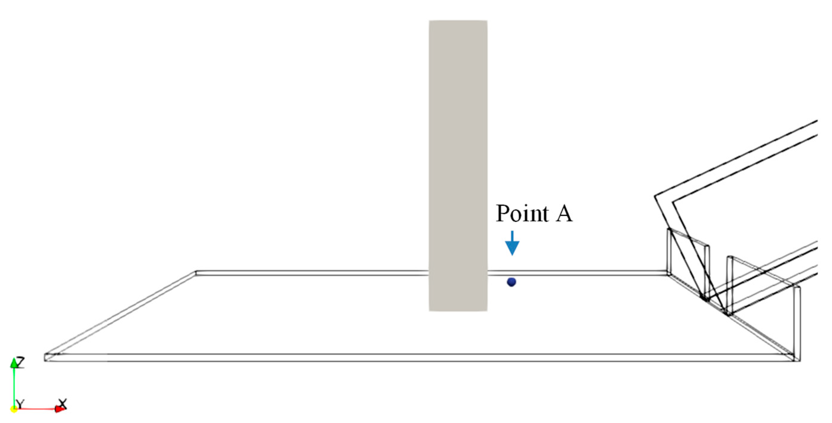
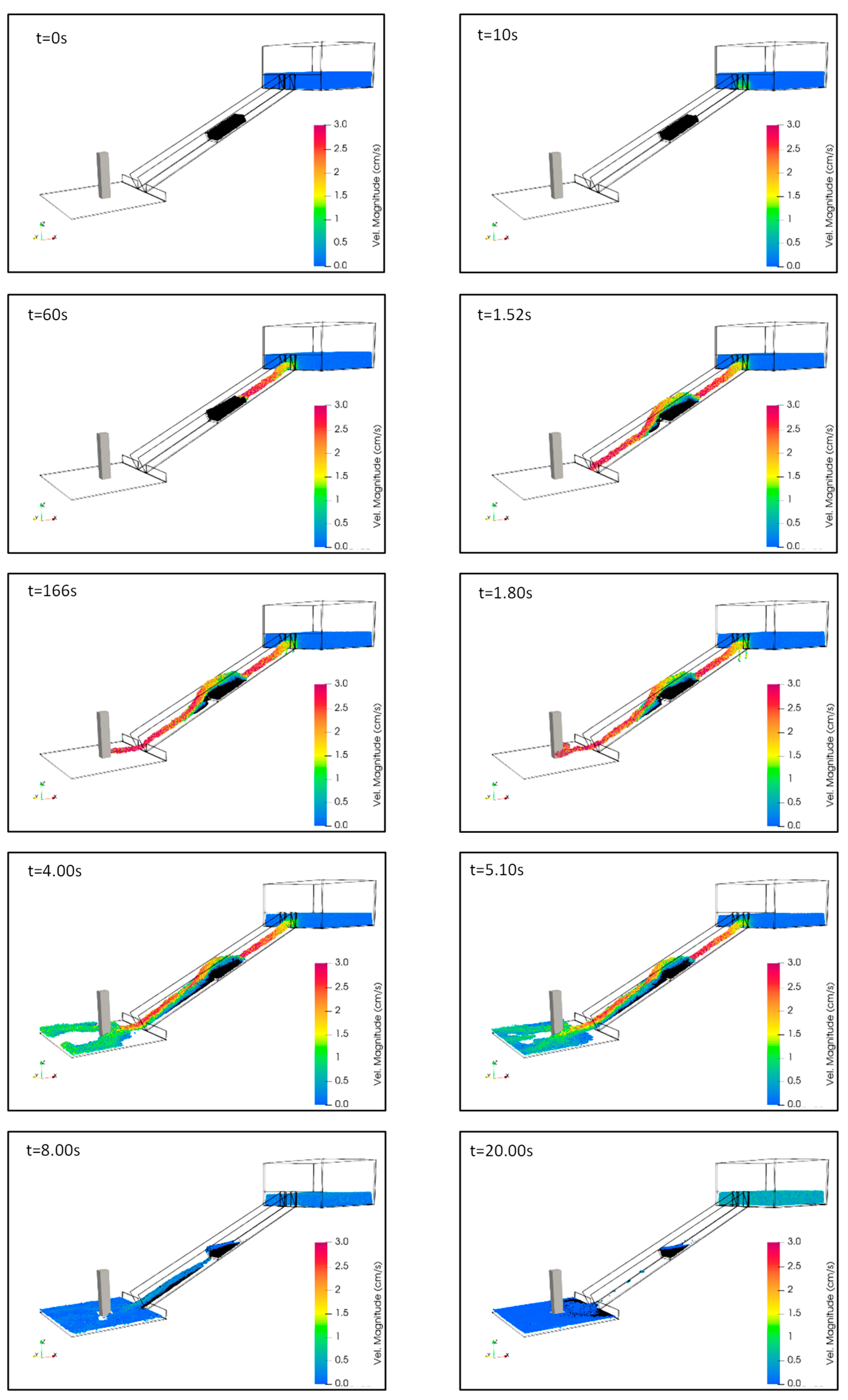
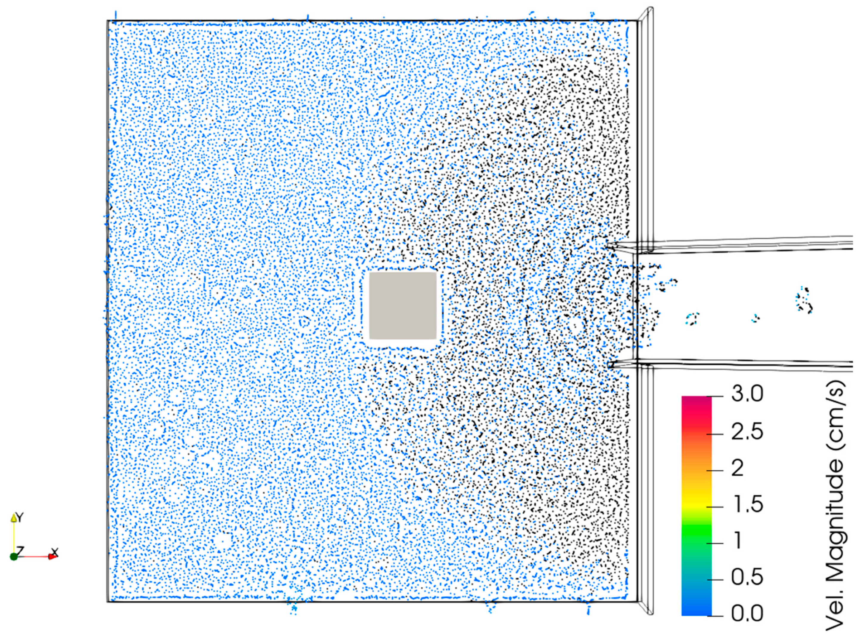
3.3. SPH Simulation on Debris Flow Impact
4. Result and Discussion
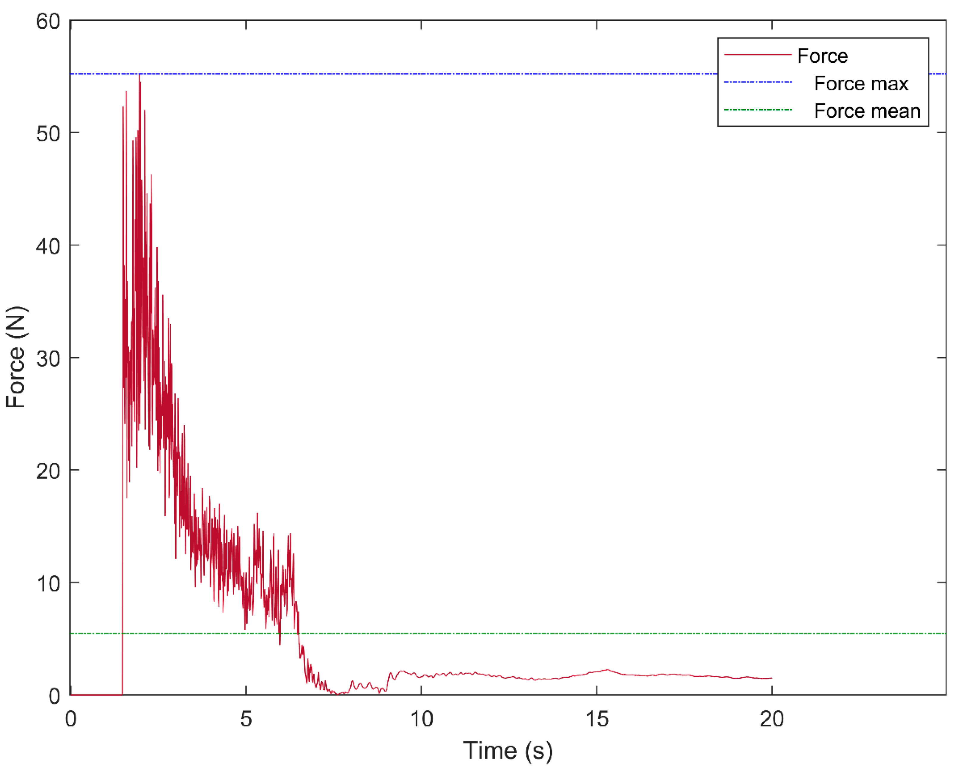
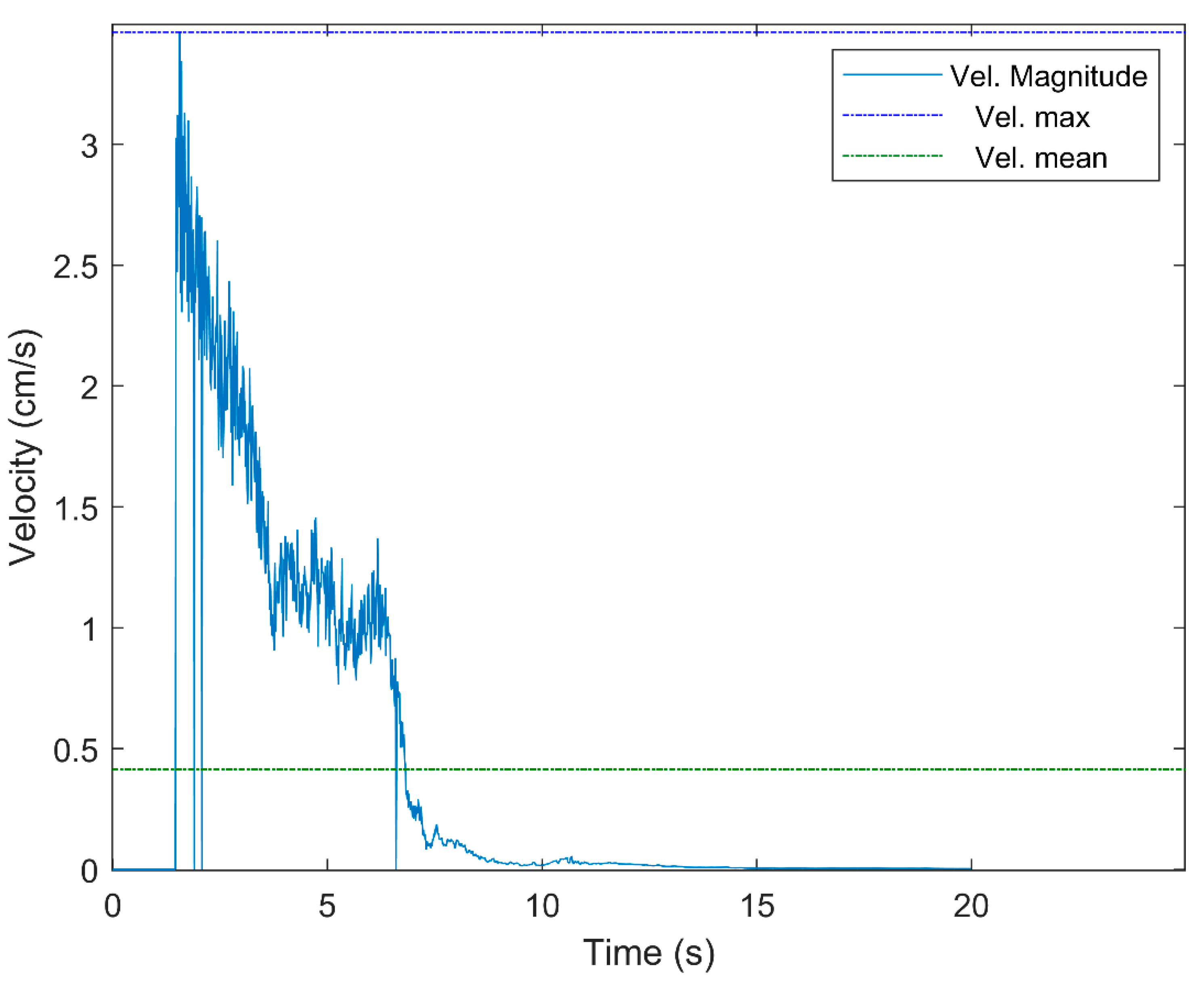
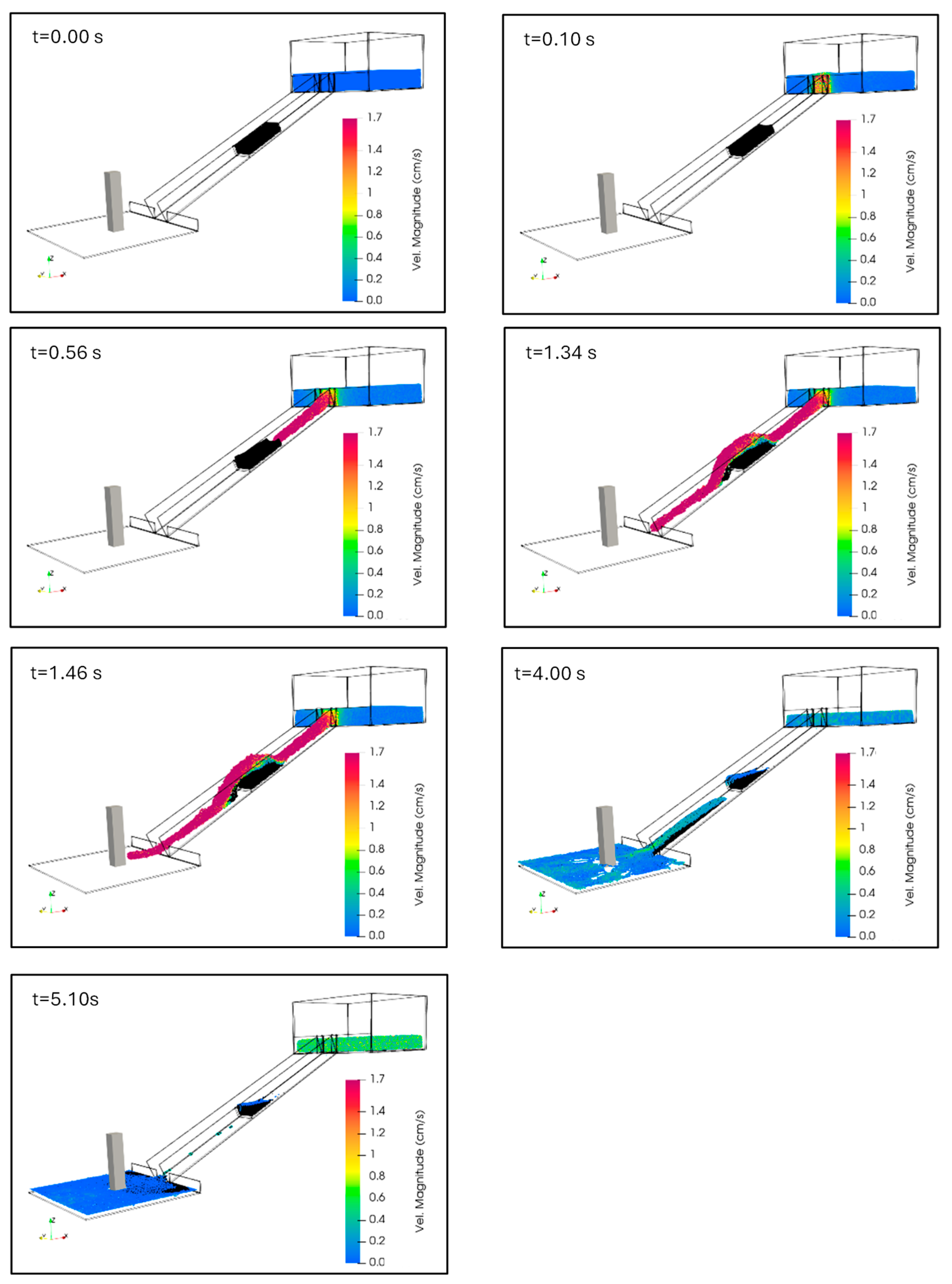
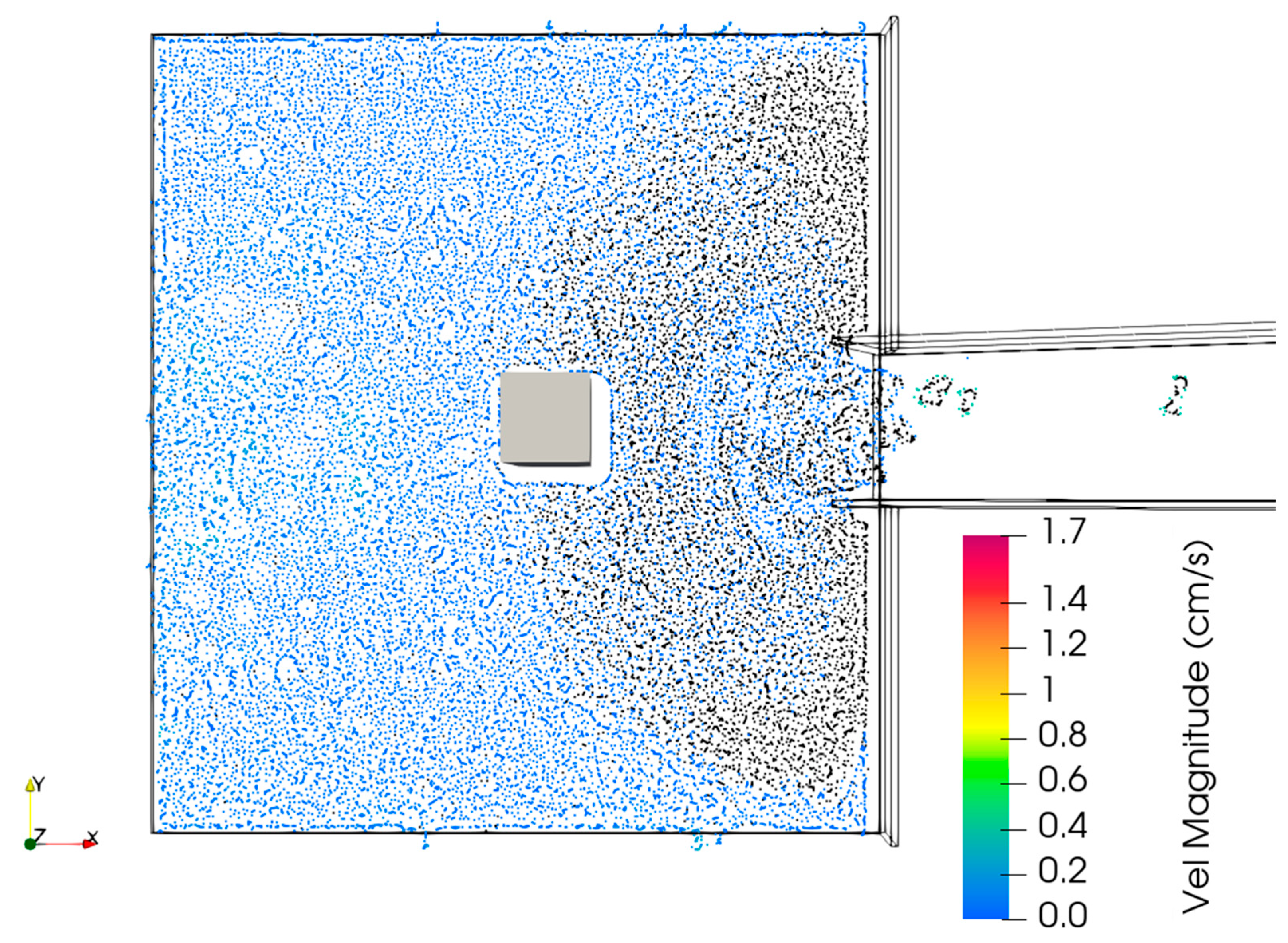
4.1. Case 1A
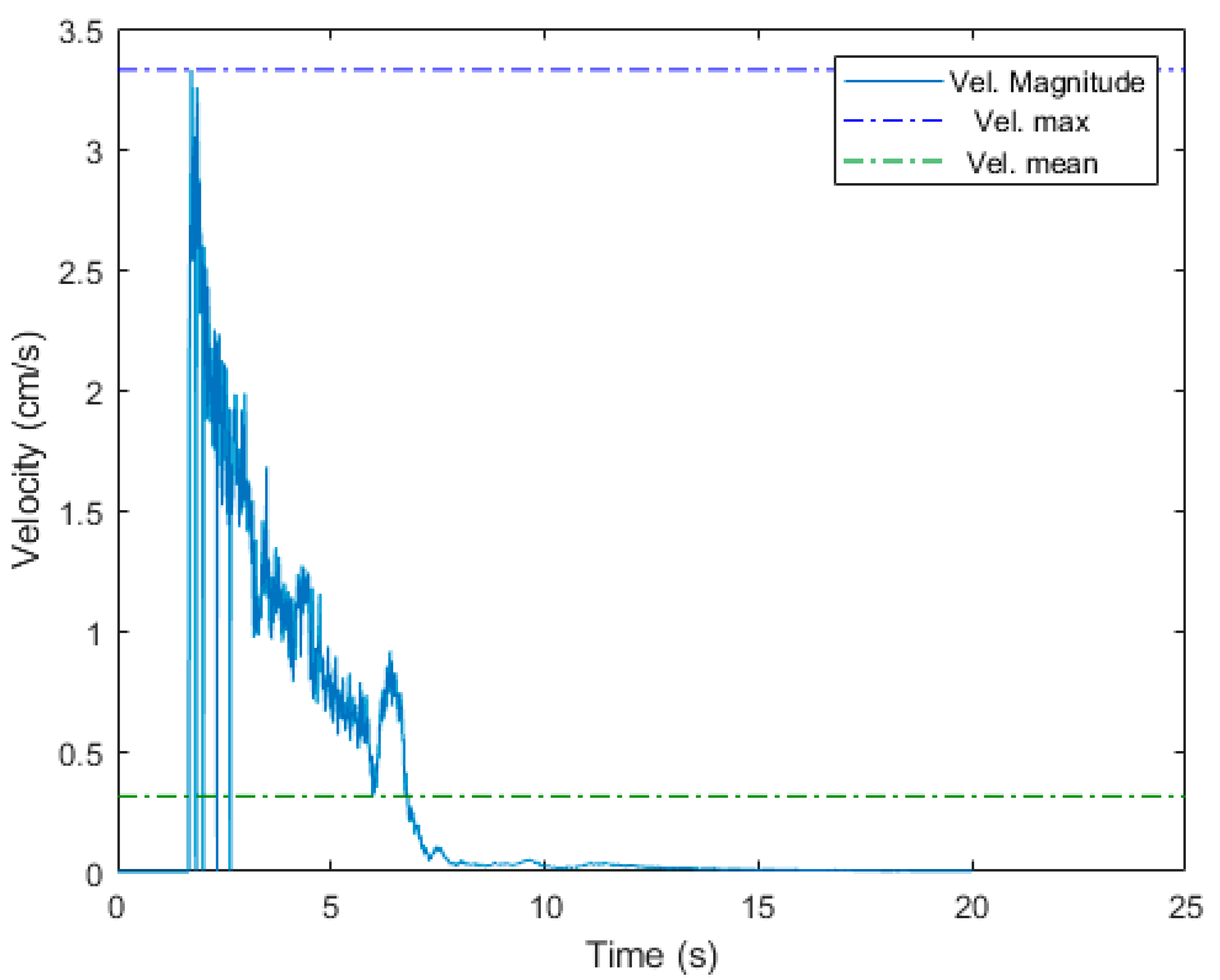
4.2. Case 1B
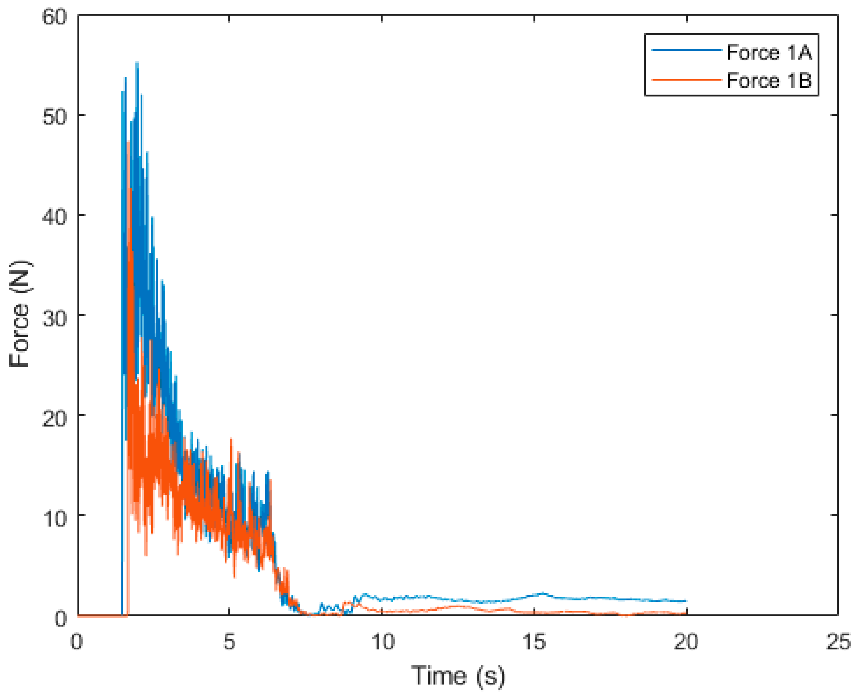
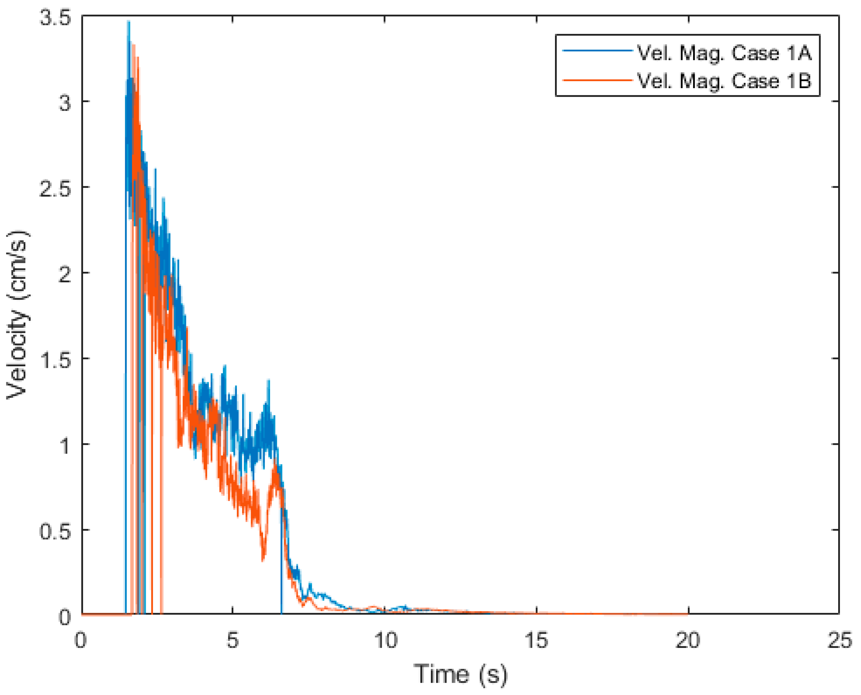
4.3. Comparison Case 1A and 1B
5. Conclusions
Author Contributions
Funding
Institutional Review Board Statement
Informed Consent Statement
Data Availability Statement
Acknowledgments
Conflicts of Interest
References
- Takahashi, T. A Review of Japanese Debris Flow Research. Int. J. Eros. Control Eng. 2009, 2, 1–14. [Google Scholar] [CrossRef]
- Zhou, G.D.; Law, R.P.H.; Ng, C.W.W. The mechanisms of debris flow: A preliminary study. In Proceedings of the 17th International Conference on Soil Mechanics and Geotechnical Engineering, Alexandria, Egypt, 5–9 October 2009; Volume 2, pp. 1570–1573. [Google Scholar] [CrossRef]
- Mohd Arif Zainol, M.R.R.; AWahab, M.K. Hydraulic Physical Model of Debris Flow for Malaysia Case Study. IOP Conf. Ser. Mater. Sci. Eng. 2018, 374. [Google Scholar] [CrossRef]
- Tiranti, D.; Crema, S.; Cavalli, M.; Deangeli, C. An Integrated Study to Evaluate Debris Flow Hazard in Alpine Environment. Front. Earth Sci. 2018, 6, 1–14. [Google Scholar] [CrossRef]
- Muhammad, N.S.; Julien, P.Y.; Salas, J.D. Probability Structure and Return Period of Multiday Monsoon Rainfall. J. Hydrol. Eng. 2016, 21, 1. [Google Scholar] [CrossRef]
- Rahman, H.A.; Mapjabil, J. Landslides Disaster in Malaysia: An Overview. Heal. Environ. J. 2017, 8, 58–71. [Google Scholar]
- Wahab, M.K.; Mohd Arif Zainol, M.R.R.; Ikhsan, J.; Zawawi, M.H.; Abas, M.A.; Mohamed Noor, N.; Abdul Razak, N.; Bhardwaj, N.; Mohamad Faudzi, S.M. Smoothed particle hydrodynamics simulation of debris flow on deposition area. Nat. Hazards 2024, 120, 12107–12136. [Google Scholar] [CrossRef]
- Joe, E., Jr.; Tongkul, F.; Roslee, R. Engineering Properties of Debris Flow Material At Bundu Tuhan, Ranau, Sabah, Malaysia. Pakistan J. Geol. 2018, 2, 22–26. [Google Scholar] [CrossRef]
- Kasim, N.; Taib, K.A.; Mukhlisin, M.; Kasa, A. Triggering Mechanism and Characteristic of Debris Flow in Peninsular Malaysia. Am. J. Enginering Res. 2016, 5, 112–119. [Google Scholar]
- Khairi, M.A.W.; Rozainy, M.R.; Ikhsan, J. Smoothed Particle Hydrodynamics Simulation for Debris Flow: A Review. IOP Conf. Ser. Mater. Sci. Eng. 2020, 864, 012045. [Google Scholar] [CrossRef]
- Liu, K.F.; Huang, M.C. Numerical simulation of debris flows. Proc. Int. Conf. Offshore Mech. Arct. Eng.—OMAE 2010, 6, 375–382. [Google Scholar] [CrossRef]
- Chang, T.C.; Wang, Z.Y.; Chien, Y.H. Hazard assessment model for debris flow prediction. Environ. Earth Sci. 2010, 60, 1619–1630. [Google Scholar] [CrossRef]
- Li, M.; Jiang, Y.; Yang, T.; Huang, Q.; Qiao, J.; Yang, Z. Early warning model for slope debris flow initiation. J. Mt. Sci. 2018, 15, 1342–1353. [Google Scholar] [CrossRef]
- Vargas-Cuervo, G.; Rotigliano, E.; Conoscenti, C. Prediction of debris-avalanches and -flows triggered by a tropical storm by using a stochastic approach: An application to the events occurred in Mocoa (Colombia) on 1 April 2017. Geomorphology 2019, 339, 31–43. [Google Scholar] [CrossRef]
- Zhou, J.W.; Cui, P.; Yang, X.G.; Su, Z.M.; Guo, X.J. Debris flows introduced in landslide deposits under rainfall conditions: The case of Wenjiagou gully. J. Mt. Sci. 2013, 10, 249–260. [Google Scholar] [CrossRef]
- Chen, S.C.; Wu, C.Y. Debris flow disaster prevention and mitigation of non-structural strategies in Taiwan. J. Mt. Sci. 2014, 11, 308–322. [Google Scholar] [CrossRef]
- Lay, U.S.; Pradhan, B. Identification of debris flow initiation zones using topographic model and airborne laser scanning data. Lect. Notes Civ. Eng. 2019, 9, 915–940. [Google Scholar] [CrossRef]
- Pradhan, B.; Bakar, S.B.A. Debris Flow Source Identification in Tropical Dense Forest Using Airborne Laser Scanning Data and Flow-R Model BT—Laser Scanning Applications in Landslide Assessment; Pradhan, B., Ed.; Springer International Publishing: Cham, Switzerland, 2017; pp. 85–112. [Google Scholar]
- Yosuke, Y.; Rozainy, M.A.Z.M.R.; Taku, M.; Tamotsu, T.; Kaoru, T. Experimental study of debris particles movement characteristics at low and high slope. J. Glob. Environ. Eng. 2012, 17, 9–18. [Google Scholar]
- Borga, M.; Stoffel, M.; Marchi, L.; Marra, F.; Jakob, M. Hydrogeomorphic response to extreme rainfall in headwater systems: Flash floods and debris flows. J. Hydrol. 2014, 518, 194–205. [Google Scholar] [CrossRef]
- Naqvi, D.K.C.M.W.; Hu, L. A Case Study and Numerical Modeling of Post-Wildfire Debris Flows in Montecito, California. Water 2024, 16, 1285. [Google Scholar] [CrossRef]
- Kean, J.W.; Staley, D.M.; Lancaster, J.T.; Rengers, F.K.; Swanson, B.J.; Coe, J.A.; Hernandez, J.L.; Sigman, A.J.; Allstadt, K.E.; Lindsay, D.N. Inundation, Flow Dynamics, and Damage in the 9 January 2018 Montecito Debris-Flow Event, California, USA: Opportunities and Challenges for Post-Wildfire Risk Assessment. Geosphere 2019, 15, 1140–1163. [Google Scholar] [CrossRef]
- Tuckett, Q.M.; Koetsier, P. Mid- And Long-Term Effects of Wildfire and Debris Flows on Stream Ecosystem Metabolism. Freshw. Sci. 2016, 35, 445–456. [Google Scholar] [CrossRef]
- Parise, M.; Cannon, S.H. Wildfire Impacts on the Processes That Generate Debris Flows in Burned Watersheds. Nat. Hazards 2011, 61, 217–227. [Google Scholar] [CrossRef]
- Zhang, J.; Guo, Z.; Wang, D.; Qian, H. The Quantitative Estimation of the Vulnerability of Brick and Concrete Building Impacted by Debris Flow. Nat. Hazards Earth Syst. Sci. Discuss. 2015, 3, 5015–5044. [Google Scholar] [CrossRef]
- Ciurean, R.L.; Hussin, H.; van Westen, C.J.; Jaboyedoff, M.; Nicolet, P.; Chen, L.; Frigerio, S.; Glade, T. Multi-Scale Debris Flow Vulnerability Assessment and Direct Loss Estimation of Buildings in the Eastern Italian Alps. Nat. Hazards 2016, 85, 929–957. [Google Scholar] [CrossRef]
- Nicolae, A.F.; Deák, G.; Tudor, G.; Cirstinoiu, C.T.; Zamfir, A.S.; Uritescu, B.; Georgescu, L.; Ghita, G.; Raischi, M.; Daescu, A.I.; et al. Comparative analysis on water velocity distribution in the context of riverbed morphology changes and discharge variation. J. Environ. Prot. Ecol. 2017, 18, 1649–1657. [Google Scholar]
- Hu, K.; Cui, P.; Zhang, J.Q. Characteristics of Damage to Buildings by Debris Flows on 7 August 2010 in Zhouqu, Western China. Nat. Hazards Earth Syst. Sci. 2012, 12, 2209–2217. [Google Scholar] [CrossRef]
- Bugnion, L.; McArdell, B.W.; Bartelt, P.; Wendeler, C. Measurements of Hillslope Debris Flow Impact Pressure on Obstacles. Landslides 2011, 9, 179–187. [Google Scholar] [CrossRef]
- Luo, H.; Zhang, L.M.; He, J.; Yin, K. Reliability-Based Formulation of Building Vulnerability to Debris Flow Impacts. Can. Geotech. J. 2022, 59, 40–54. [Google Scholar] [CrossRef]
- Kang, H.-G.; Kim, Y.-T. Physical Vulnerability Function of Buildings Impacted by Debris Flow. Korean Soc. Hazard Mitig. 2014, 14, 133–143. [Google Scholar] [CrossRef]
- Liu, X.; Wang, F.; Nawnit, K.; Lv, X.; Wang, S. Experimental study on debris flow initiation. Bull. Eng. Geol. Environ. 2020, 79, 1565–1580. [Google Scholar] [CrossRef]
- Zhuang, J.; Cui, P.; Peng, J.; Hu, K.; Iqbal, J. Initiation process of debris flows on different slopes due to surface flow and trigger-specific strategies for mitigating post-earthquake in old Beichuan County, China. Environ. Earth Sci. 2013, 68, 1391–1403. [Google Scholar] [CrossRef]
- Yamashiki, Y.; Rozainy, M.A.Z.M.R.; Matsumoto, T.; Takahashi, T.; Takara, K. Particle Routing Segregation of Debris Flow Mechanisms Near the Erodible Bed. APCBEE Procedia 2013, 5, 527–534. [Google Scholar] [CrossRef]
- Dai, Z.; Wang, F.; Huang, Y.; Song, K.; Iio, A. SPH-based numerical modeling for the post-failure behavior of the landslides triggered by the 2016 Kumamoto earthquake. Geoenvironmental Disasters 2016, 3, 24. [Google Scholar] [CrossRef]
- Liu, G.-R.; Liu, M.B. Smoothed Particle Hydrodynamics: A Meshfree Particle Method; World Scientific Publishing Co. Pte. Ltd: Singapore, 2010. [Google Scholar]
- Liu, M.B.; Liu, G. Smoothed particle hydrodynamics (SPH): An overview and recent developments. Arch. Comput. methods Eng. 2010, 17, 25–76. [Google Scholar] [CrossRef]
- Gomez-Gesteira, M.; Rogers, B.D.; Crespo, A.J.C.; Dalrymple, R.A.; Narayanaswamy, M.; Dominguez, J.M. SPHysics—development of a free-surface fluid solver—Part 1: Theory and formulations. Comput. Geosci. 2012, 48, 289–299. [Google Scholar] [CrossRef]
- Li, B.; Fang, Y.; Li, Y.; Zhu, C. Dynamics of Debris Flow-Induced Impacting Onto Rigid Barrier With Material Source Erosion-Entrainment Process. Front. Earth Sci. 2023, 11, 1132635. [Google Scholar] [CrossRef]
- Li, B.; Wang, C.; Li, Y.; Zhang, S. Dynamic Response Study of Impulsive Force of Debris Flow Evaluation and Flexible Retaining Structure Based on SPH-DEM-FEM Coupling. Adv. Civ. Eng. 2021, 2021, 098250. [Google Scholar] [CrossRef]
- Zhao, H.; Yao, L.; You, Y.; Wang, B.; Zhang, C. Experimental Study of the Debris Flow Slurry Impact and Distribution. Shock Vib. 2018, 2018, 460362. [Google Scholar] [CrossRef]
- Yang, X.F.; Peng, S.L.; Liu, M.B. A new kernel function for SPH with applications to free surface flows. Appl. Math. Model. 2014, 38, 3822–3833. [Google Scholar] [CrossRef]
- Zhang, Z.; Zhang, W.; Zhai, Z.J.; Chen, Q.Y.; Zhai, Z.J.; Chen, Q.Y. Evaluation of Various Turbulence Models in Predicting Airflow and Turbulence in Enclosed Environments by CFD: Part 2—Comparison with Experimental Data from Literature. HVAC&R Res. 2007, 13, 871–886. [Google Scholar]
- Tudor, G.; György, D.; Cirstinoiu, C.; Raischi, M.; Danalache, T.; Cornateanu, G.; Bratfanof, E. Transboundary River Hydrodynamic Conditions Assessment in Sustainable Development Context. A Case Study of Danube River: Chilia Branch—Bystroe Channel Area. IOP Conf. Ser. Earth Environ. Sci. 2020, 616, 012072. [Google Scholar] [CrossRef]


| Category | Range (%) | Quality |
|---|---|---|
| A | <10 | Good |
| B | 10–30 | Acceptable |
| C | 30–40 | Marginal |
| D | 50> | Poor |
| Case Study | Flume Degree (°) | Water Level (mm) | Gate Opening |
|---|---|---|---|
| 1 | 15 | 120 | Half |
| 2 | 15 | 120 | Full |
| 3 | 15 | 150 | Half |
| 4 | 15 | 150 | Full |
| 5 | 20 | 120 | Half |
| 6 | 20 | 120 | Full |
| 7 | 20 | 150 | Half |
| 8 | 20 | 150 | Full |
| 9 | 25 | 120 | Half |
| 10 | 25 | 120 | Full |
| 11 | 25 | 150 | Half |
| 12 | 25 | 150 | Full |
| Case No. | Planar Area (mm2) | Relative Error (%) | |
|---|---|---|---|
| Experimental (×103) | SPH (×103) | ||
| 1 | 536.79 | 594.78 | 10.25 |
| 2 | 436.93 | 450.14 | 2.98 |
| 3 | 488.42 | 547.41 | 11.39 |
| 4 | 402.34 | 451.66 | 11.55 |
| 5 | 461.38 | 519.03 | 11.76 |
| 6 | 447.06 | 493.72 | 9.92 |
| 7 | 415.86 | 462.13 | 10.54 |
| 8 | 290.03 | 320.00 | 9.83 |
| 9 | 367.62 | 408.24 | 7.51 |
| 10 | 321.46 | 364.98 | 12.68 |
| 11 | 485.07 | 550.74 | 14.05 |
| 12 | 298.70 | 331.70 | 10.47 |
| Case | Slope Angle (°) | Water Level in Water Tank (m) | Water Gate Operation | Water Gate Open Time (s) | Total Elements | Simulation Runtime (HH:MM:SS) | Time of Simulation (s) |
|---|---|---|---|---|---|---|---|
| 1A | 25 | 0.2 | Fully Open | 5 | 500,899 | 1:19:33 | 20 |
| 1B | 25 | 0.2 | Half Open | 5 | 500,899 | 1:25:55 | 20 |
| Case | Force | Vel. Magnitude | ||||
|---|---|---|---|---|---|---|
| Max. (N) | Mean (N) | Mean Percentage Difference (%) | Max. (cm/s) | Mean (cm/s) | Mean Percentage Difference (%) | |
| 1A | 55.2 | 5.45 | 50.86 | 3.44 | 0.41 | 27.78 |
| 1B | 47.3 | 3.24 | 3.33 | 0.31 | ||
Disclaimer/Publisher’s Note: The statements, opinions and data contained in all publications are solely those of the individual author(s) and contributor(s) and not of MDPI and/or the editor(s). MDPI and/or the editor(s) disclaim responsibility for any injury to people or property resulting from any ideas, methods, instructions or products referred to in the content. |
© 2025 by the authors. Licensee MDPI, Basel, Switzerland. This article is an open access article distributed under the terms and conditions of the Creative Commons Attribution (CC BY) license (https://creativecommons.org/licenses/by/4.0/).
Share and Cite
Wahab, M.K.A.; Zainol, M.R.R.M.A.; Abas, M.A.; Razak, N.A. Numerical Analysis of Debris Impact Forces and Its Environmental Repercussions Using Smoothed Particle Hydrodynamics. Environ. Earth Sci. Proc. 2025, 33, 7. https://doi.org/10.3390/eesp2025033007
Wahab MKA, Zainol MRRMA, Abas MA, Razak NA. Numerical Analysis of Debris Impact Forces and Its Environmental Repercussions Using Smoothed Particle Hydrodynamics. Environmental and Earth Sciences Proceedings. 2025; 33(1):7. https://doi.org/10.3390/eesp2025033007
Chicago/Turabian StyleWahab, Muhammad Khairi A., Mohd Remy Rozainy Mohd Arif Zainol, Mohamad Aizat Abas, and Norizham Abdul Razak. 2025. "Numerical Analysis of Debris Impact Forces and Its Environmental Repercussions Using Smoothed Particle Hydrodynamics" Environmental and Earth Sciences Proceedings 33, no. 1: 7. https://doi.org/10.3390/eesp2025033007
APA StyleWahab, M. K. A., Zainol, M. R. R. M. A., Abas, M. A., & Razak, N. A. (2025). Numerical Analysis of Debris Impact Forces and Its Environmental Repercussions Using Smoothed Particle Hydrodynamics. Environmental and Earth Sciences Proceedings, 33(1), 7. https://doi.org/10.3390/eesp2025033007