Assessment of Machine Learning Techniques to Estimate Reference Evapotranspiration at Yauri Meteorological Station, Peru ^†

Abstract

Reference evapotranspiration (ETo) is crucial for agriculture and is traditionally estimated using the Penman–Monteith (PM) method, which relies on multiple climatic variables. This study assessed machine learning (ML) techniques to estimate ETo at the Yauri meteorological station in Peru. Two ML models—K-nearest neighbors (KNN) and artificial neural networks (ANN)—were tested and compared against both the PM and the Hargreaves–Samani (HS) methods. Their accuracy was measured using metrics such as mean absolute error (MAE), anomaly correlation coefficient (ACC), Nash–Sutcliffe efficiency (NSE), Kling–Gupta efficiency (KGE), and spectral angle (SA). The results indicate that ML techniques can effectively estimate ETo, providing robust alternatives in areas with limited meteorological data, thus enhancing water resource management.

1. Introduction

The consumptive use of water, or evapotranspiration (ET), is one of the basic components of the hydrological cycle [1] and is a key driver for agriculture, irrigation scheduling, and water resources [2]. Since it is difficult to determine the ET for each crop, the reference evapotranspiration (ETo) is calculated, and then the ET is estimated using ETo [3]. The main climatic variables to estimate ETo are air temperature, solar radiation, relative humidity, and wind speed [4]. The most accurate means of estimating ETo is by applying methods that consider all the primary factors that affect the ETo rate, such as the standard Penman–Monteith (PM) method. The precision of the estimates depends substantially on the quality of the data and the integrity and physical basis of the method [1]. The reliable quantification of ETo is essential for estimating the net irrigation requirement, planning and management of water resources, and modeling the effect of climate change [5].

Several empirical models have been developed to estimate ETo; however, performance can be significantly dependent on location and local recalibration. PM, presented by [4], is considered the only reference method to determine ETo; however, the method requires a large amount of input data, which is not always accessible [6,7]. Thus, the choice of a method depends on the availability of quality meteorological data, as well as the accuracy and precision of the model estimates for a given region [8].

The PM equation has been widely used to calibrate and validate other methods to estimate ETo [3,9,10]. Another method widely used in different studies, with reliable results and with the use of less meteorological data (solar radiation and temperature), is the Hargreaves–Samani method [11]; however, its level of performance to estimate ETo in a given place essentially depends on the proper calibration of the coefficients according to local conditions.

In recent years, the use of artificial intelligence (AI) techniques has shown satisfactory results in different fields of engineering, biomedical, economic, and social. These applications provide more robust and efficient models that can learn complex systems. Machine learning (ML) algorithms as part of AI have been used in ET estimation [10,12] and wind power forecasting [13].

The objective of this study was to assess machine learning techniques to estimate reference evapotranspiration at the Yauri meteorological station in Peru, evaluating their accuracy and reliability as alternatives for regions with limited data and supporting improved water resource management.

2. Materials and Methods

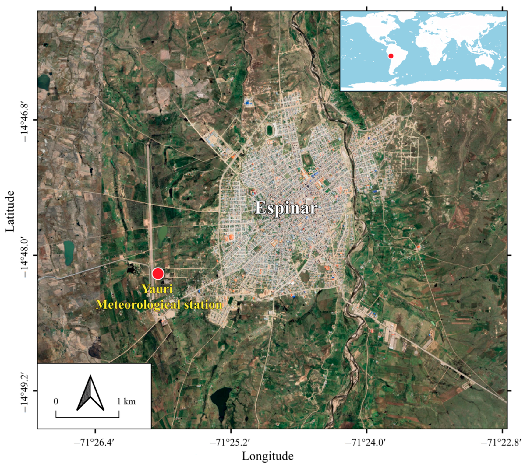
2.1. Study Area

The study was conducted at the Yauri meteorological station in Espinar, Cusco, within the upper Apurimac river basin (14° 48′ 5” S, 71° 25′ 54” W, 3927 m a.s.l.) (Figure 1). The area has a semi-arid climate according to the Thornthwaite classification [14]. Annual average precipitation is 809.6 mm, mostly concentrated in summer (60.7% from December to February). Autumn contributes 23.7% of rainfall, mainly in March, with winter and spring receiving 1.4% and 14.2%, respectively. Average temperatures are 17.2 °C (maximum), 8.0 °C (mean), and −1.7 °C (minimum), with sub-zero temperatures in winter. July is the coldest month (average minimum. −8.6 °C), while spring sees maximums above 18 °C.

The dataset was obtained from a meteorological station operated by the Servicio Nacional de Meteorología e Hidrología (SENAMHI) of Peru, covering a monthly timespan from January 2000 to December 2014. The station recorded maximum air temperature (Tx, °C), minimum air temperature (Tn, °C), wind speed (U, m/s), relative humidity (RH, %), and sunshine hours (SH, h). Wind speed measurements at 10 m (U) were adjusted to 2 m (U₂), and extraterrestrial solar radiation (Ro, mm/d) was calculated as per [4] guidelines. The 15-year dataset comprised 180 records for each variable. The data were randomly split, with 70% used for model training and 30% for validation.

2.2. Standard Estimated of ETo

The FAO-56 Penman–Monteith equation was used as the global standard method to estimate the ETo, considered the most accurate method, being the daily form of the equation according to the Irrigation and Drainage Manual 56 of FAO as follows ([4] Allen et al., 1998):

$${ET}_{O,PM}={\displaystyle \frac{0.408\Delta \left(R_n-G\right)+\gamma \frac{900}{T_m+273}{U}_2(e_s-e_a)}{\Delta +\gamma (1+0.34u_2)}}$$

(1)

where ${ET}_{O,PM}$ is reference evapotranspiration (mm/d), ∆ is the slope of the vapor pressure curve (Kpa/°C), Rn is the net radiation on the crop surface (MJ/m²/d), G is the heat of the soil flux density on the soil surface (MJ/m²/d), γ is the psychrometric constant (kPa/°C), Tm is the mean daily air temperature (°C), $U_2$ is the mean daily wind speed at 2 m altitude (m/s), $e_s$ is the saturation vapor pressure (kPa), $e_a$ is the real vapor pressure (kPa), and $e_s-e_a$ is the saturation vapor pressure deficit (kPa).

2.3. Hargreaves–Samani Method

The estimate of ETo by applying the Hargreaves–Samani (HS) method [11], is determined according to the following equation:

$${ET}_{O,HS}=0.0023·R_a(Tm+17.8){\left(Tx-Tn\right)}^{0.5}$$

(2)

where ${ET}_{O,HS}$ is the reference evapotranspiration (mm/d) estimated by the HS equation; Ra is the extraterrestrial radiation (mm/d); and Tx, Tn, and Tm are daily maximum and minimum temperature and mean air temperature (°C), with Tm calculated as the average of Tx and Tn.

2.4. Machine Learning Algorithms

Two ML algorithms based on supervised learning [15] were trained and validated: K-nearest neighbors (KNN) and artificial neural networks (ANN).

2.4.1. K-Nearest Neighbors (KNN) Algorithm

KNN, a simple non-parametric method, does not assume a functional relationship between the input and output [16] and is widely used for classification and regression [17,18]. The output is the average of the k nearest neighbors:

$$\widehat{y}={\displaystyle \frac{\left(\sum _{i=1}^k{y}_i\right)}{k}}$$

(3)

where $\widehat{y}$ is the output value, $k$ is the number of nearest neighbors, and $y_i$ is the ith nearest neighbor. The method uses Euclidean distance to compute the similarity between instances [2]. In this study, $k$ varied from 2 to 4, with the optimal value selected based on the highest Nash–Sutcliffe efficiency (NSE) and lowest mean absolute error (MAE). To maintain consistency in the analysis, an average value of k = 3 was used.

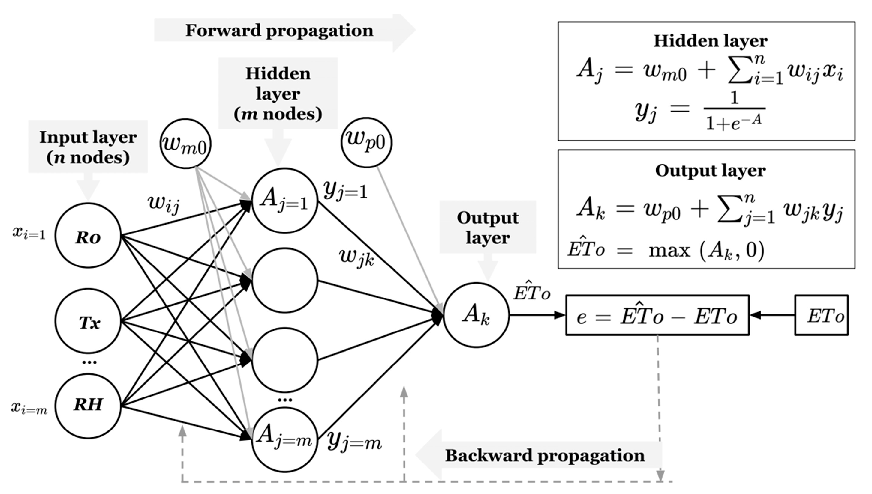
2.4.2. Artificial Neural Network (ANN)

ANNs are computational models that simulate biological neurons, enabling complex calculations [19]. This study uses the Multilayer Perceptron Neural Network (MPNN), which is commonly applied in prediction and regression tasks [20] and widely used in water resources [21,22].

The MPNN architecture consists of input, hidden, and output layers, with weights determining the output values. Error adjustments are made through backpropagation using gradient descent [23]. The number of neurons in the input layer corresponds to the number of variables, which are processed through successive layers to the output layer, where the target variable is obtained [24]. A single hidden layer can solve most problems with enough hidden units [25,26]. MPNN can approximate non-linear functions using sigmoid and linear activation functions in the hidden and output layers, respectively [25]. The process iterates through forward and backward propagation until the error is minimized [23].

Figure 2 shows the typical architecture of the MPNN and its simplified mathematical formulation. The MPNN used includes an input layer, a hidden layer, and an output layer. Given the dataset’s varying scales and large values for ETo estimation, features were standardized to resemble a Gaussian distribution ($u=0$ and $s=1$), a common requirement for many ML estimators [27]. The standard score (z-score) of the input samples was calculated as follows:

$$z={\displaystyle \frac{\left(x-u\right)}{s}}$$

(4)

where $u$ is the mean, and $s$ is the standard deviation of the training samples.

In the hidden layer, each neuron ($A_j$) performs a linear weighted sum process between the coefficients ($w_{ij}$) and the neurons of the input layer ($R_o,Tx,\dots ,RH$) plus a bias ($w_{m0}$). The outputs of each neuron of the hidden layer ($y_j$) are calculated by means of a sigmoid non-linear activation function, which was selected due to its ability to introduce non-linearity into the model, allowing it to capture complex relationships between input variables. In the same way as the output layer, the neuron ($A_k$) performs a linear combination process between the coefficients ($w_{jk}$) and the neurons of the hidden layer ($y_j$) plus a bias ($w_{p0}$).

The output neuron (${\widehat{ET}}_o$) was computed using a rectified linear unit (ReLU) activation function to ensure non-negative estimates in accordance with the physical nature of ETo. Multilayer neural networks, also known as feedforward networks, feed signals from the input to the output layer, with each node connected to the next layer’s nodes. The model’s performance is optimized using a loss function in the output layer [28].

In this study, the mean squared error (MSE) loss function was used due to its sensitivity to large errors, allowing for more stable convergence during training. During forward propagation, input signals pass through the network layers until the final prediction is obtained [16]. The network was trained using backpropagation, adjusting the weights with the Adam optimization algorithm, which combines momentum and adaptive learning rates to improve convergence speed and avoid local minima.

2.5. Model Development

Different combinations of five climatic variables were explored as inputs to estimate ETo: Ro, Tx, Tn, U₂, SH, and RH. A correlation matrix was developed to understand which climatic variables have the best relationships with ETo.

Table 1. Input combinations of the KNN and ANN models.

Combination	Models		Input Combinations
1	KNN1	ANN1	${ET}_o=f(Ro,Tx,Tn,U_2,SH,RH)$
2	KNN2	ANN2	${ET}_o=f(Ro,Tx,Tn)$
3	KNN3	ANN3	${ET}_o=f(Ro,Tx)$

shows different input combinations for the used models.

2.6. Goodness-of-Fit Metrics

Five performance metrics (

Table 2. Goodness-of-fit metrics.

Metrics	Equation 1	Optimal Value
Anomaly correlation coefficient (ACC)	$ACC={\displaystyle \frac{1}{n}}{\displaystyle \frac{\left(\sum _{i=1}^n(S_i-\overline{S})\right(O_i-\overline{O})}{{\sigma }_O{\sigma }_S}}$	±1
Nash–Sutcliffe Efficiency (NSE)	$NSE=1-{\displaystyle \frac{\sum _{i=1}^n{(S_i-O_i)}^2}{\sum _{i=1}^n{(O_i-\overline{O})}^2}}$	1
Kling–Gupta efficiency (KGE’)	${KGE}^{\prime }=\sqrt{{\left(r-1\right)}^2+{{\left(\beta -1\right)}^2+\left(\gamma -1\right)}^2}$ $\beta ={\displaystyle \frac{{\mu }_S}{{\mu }_O}};\gamma ={\displaystyle \frac{{CV}_S}{{CV}_O}}={\displaystyle \frac{\raisebox{1ex}{${\sigma }_S$}\!\left/ \!\raisebox{-1ex}{${\mu }_S$}\right.}{\raisebox{1ex}{${\sigma }_O$}\!\left/ \!\raisebox{-1ex}{${\mu }_O$}\right.}}$	1
Mean absolute error (MAE)	$MAE={\displaystyle \frac{1}{n}}{\displaystyle \sum _{i=0}^n}\left|S_i-O_i\right|$	0
Spectral angle (SA)	$SA=arcos\left({\displaystyle \frac{〈S,O〉}{{‖S‖}_2{‖O‖}_2}}\right)$	0

¹ Variables: $S$ is the simulated value; $\overline{S}$ is the mean of the simulated values; $O$ is the observed value; $\overline{O}$ is the mean of the observed value; $r$ is the correlation coefficient between the simulated and observed value (dimensionless); $\sigma$ is the standard deviation; $\beta$ is the bias ratio (dimensionless); $\mu$ is the mean value; $\gamma$ is the variability ratio (dimensionless); $CV$ is the coefficient of variation (dimensionless).

) were used to evaluate the simulated values from the KNN and ANN models: anomaly correlation coefficient (ACC), Nash–Sutcliffe efficiency (NSE) [29], Kling–Gupta efficiency (KGE’) [30], mean absolute error (MAE), and spectral angle (SA). The analysis was conducted using Python version 3.12.8 in the Jupyter Notebook IDE, along with the hydrostats package, which provides a comprehensive set of metrics to quantify the errors between observed and simulated time series [31].

3. Results and Discussion

High correlations with ETo were observed for Ro (r = 0.84), Tx (r = 0.77), and Tn (r = 0.57), while lower correlations were found with U₂ (r = 0.46), SH (r = −0.26), and RH (r = −0.13) (Figure 3). Consequently, Ro, Tx, and Tn emerged as the most significant variables for estimating ETo in this zone.

Model 1, with the full set of input variables, demonstrates the best performance when using ANN, showcasing excellent agreement between simulated and observed ETo values. In contrast, KNN exhibits lower predictive accuracy for this model. Model 2, which uses a reduced set of inputs, maintains high accuracy for both ANN and KNN, with KNN slightly outperforming ANN in this scenario. Model 3, which relies on the fewest input variables, shows results similar to Model 2 for ANN, while KNN’s accuracy decreases slightly. Finally, HS shows lower performance compared to the ML models across all metrics, highlighting its limitations in estimating ETo in this study (Figure 4).

The box plots in Figure 5 illustrate the distribution of residuals for the models across three different input scenarios. In Model 1 (Figure 5a), ANN shows the narrowest residual distribution, mostly within ±0.1 mm/d, indicating higher accuracy and less bias compared to KNN, which exhibits a wider range of residuals from −0.5 to 0.6 mm/d. In Model 2 (Figure 5b), the residuals for ANN extend over a broader range of approximately ±0.4 mm/d, while KNN shows a narrower spread, ranging between −0.2 and 0.4 mm/d. Finally, in Model 3 (Figure 5c), both ANN and KNN display residuals ranging between −0.4 and 0.4 mm/d. In contrast, the HS model consistently shows larger negative residuals across all three panels, suggesting a tendency to underestimate ETo values.

ML algorithms prove to be effective tools for estimating ETo. Increasing the number of input variables generally leads to more accurate results that are consistent with the PM approach. However, our findings indicate that reliable ETo estimates can still be achieved using ML models with only extraterrestrial solar radiation and temperature data. Models 2 and 3 align with the approach suggested by [11], demonstrating that using fewer meteorological inputs can be a viable alternative when comprehensive data are unavailable.

4. Conclusions

The KNN and ANN models were assessed using three distinct combinations of meteorological input variables. Their performance was compared to both the PM method and the HS model to assess their effectiveness under varying levels of data availability. Overall, both ANN and KNN demonstrated superior accuracy in estimating ETo compared to the HS model, confirming their reliability as alternative approaches, especially in data-scarce conditions.

Specifically, when Ro, Tx, and Tn were available, KNN outperformed ANN, achieving the highest accuracy and efficiency metrics compared to the reference PM method. In contrast, when only Ro and Tx were available, ANN yielded better performance than KNN. These findings highlight the importance of selecting the appropriate ML model based on data availability, ensuring more accurate ETo estimates for improved water resource management.

References

1. Jensen, M.E.; Allen, R.G. Evaporation, Evapotranspiration, and Irrigation Water Requirements: Task Committee on Revision of Manual 70; American Society of Civil Engineers (ASCE): Reston, VA, USA, 2016. [Google Scholar] [CrossRef]
2. Feng, K.; Tian, J. Forecasting reference evapotranspiration using data mining and limited climatic data. Eur. J. Remote Sens. 2021, 54, 363–371. [Google Scholar] [CrossRef]
3. Mehdizadeh, S. Estimation of daily reference evapotranspiration (ETo) using artificial intelligence methods: Offering a new approach for lagged ETo data-based modeling. J. Hydrol. 2018, 559, 794–812. [Google Scholar] [CrossRef]
4. Allen, R.G.; Pereira, L.S.; Rae, S.D.; Smith, M. Crop Evapotranspiration: Guidelines for Computing Crop Water Requirements; FAO Irrigation and drainage paper 56; FAO: Rome, Italy, 1998. [Google Scholar]
5. Pandey, P.K.; Dabral, P.P.; Pandey, V. Evaluation of reference evapotranspiration methods for the northeastern region of India. Int. Soil Water Conserv. Res. 2016, 4, 52–63. [Google Scholar] [CrossRef]
6. Lavado, W.; Lhomme, J.; Labat, D.; Loup Guyot, J.; Boulet, G. Estimación de la evapotranspiración de referencia (FAO Penman-Monteith) con limitados datos climáticos en la Cuenca Andina Amazónica Peruana. Rev. Peru. Geo-Atmos. 2015, 4, 34–36. [Google Scholar]
7. Chen, D.; Gao, G.; Xu, C.Y.; Guo, J.; Ren, G. Comparison of the Thornthwaite method and pan data with the standard Penman-Monteith estimates of reference evapotranspiration in China. Clim. Res. 2005, 28, 123–132. [Google Scholar] [CrossRef]
8. De Carvalho Alves, M.; De Carvalho, L.G.; Vianello, R.L.; Sediyama, G.C.; De Oliveira, M.S.; De Sá Junior, A. Geostatistical improvements of evapotranspiration spatial information using satellite land surface and weather stations data. Theor. Appl. Climatol. 2013, 113, 155–174. [Google Scholar] [CrossRef]
9. Antonopoulos, V.Z.; Antonopoulos, A.V. Daily reference evapotranspiration estimates by artificial neural networks technique and empirical equations using limited input climate variables. Comput. Electron. Agric. 2017, 132, 86–96. [Google Scholar] [CrossRef]
10. Granata, F. Evapotranspiration evaluation models based on machine learning algorithms: A comparative study. Agric. Water Manag. 2019, 217, 303–315. [Google Scholar] [CrossRef]
11. Hargreaves, G.H.; Samani, Z.A. Reference Crop Evapotranspiration from Temperature. Appl. Eng. Agric. 1985, 1, 96–99. [Google Scholar] [CrossRef]
12. Xu, T.; Guo, Z.; Liu, S.; He, X.; Meng, Y.; Xu, Z.; Song, L. Evaluating Different Machine Learning Methods for Upscaling Evapotranspiration from Flux Towers to the Regional Scale. J. Geophys. Res. Atmos. 2018, 123, 8674–8690. [Google Scholar] [CrossRef]
13. Demolli, H.; Dokuz, A.S.; Ecemis, A.; Gokcek, M. Wind power forecasting based on daily wind speed data using machine learning algorithms. Energy Convers. Manag. 2019, 198, 111823. [Google Scholar] [CrossRef]
14. Castro, A.; Dávila, C.; Laura, W.; Cubas Saucedo, F.; Ávalos, G.; López, C.; Villena, D.; Valdez, M.; Urbiola, J.; Trebejo, I.; et al. Climas del Perú: Mapa de Clasificación Climática Nacional; SENAMHI: Lima, Peru, 2021. [Google Scholar]
15. Igual, L.; Segui, S. Introduction to Data Science: A Python Approach to Concepts, Techniques and Applications; Springer International Publishing: Cham, Switzerland, 2020. [Google Scholar] [CrossRef]
16. Joshi, A.V. Machine Learning and Artificial Intelligence; Springer: Cham, Switzerland, 2020. [Google Scholar] [CrossRef]
17. Cover, T.; Hart, P. Nearest neighbor pattern classification. IEEE Trans. Inf. Theory. 1967, 13, 21–27. [Google Scholar] [CrossRef]
18. Wu, X.; Kumar, V.; Ross Quinlan, J.; Ghosh, J.; Yang, Q.; Motoda, H.; MCLachlan, G.J.; Ng, A.; Liu, B.; Yu, P.S.; et al. Top 10 Algorithms in Data Mining. Knowl. Inf. Syst. 2008, 14, 1–37. [Google Scholar] [CrossRef]
19. Shalev-Shwartz, S.; Ben-David, S. Understanding Machine Learning: From Theory to Algorithms; Cambridge University Press: Cambridge, UK, 2014. [Google Scholar]
20. Rumelhart, D.E.; Hinton, G.E.; Williams, R.J. Learning representations by back-propagating errors. Nature 1986, 323, 533–536. [Google Scholar] [CrossRef]
21. Maier, H.R.; Dandy, G.C. Neural networks for the prediction and forecasting of water resources variables: A review of modelling issues and applications. Environ. Model. Softw. 2000, 15, 101–124. [Google Scholar] [CrossRef]
22. Maier, H.R.; Jain, A.; Dandy, G.C.; Sudheer, K.P. Methods used for the development of neural networks for the prediction of water resource variables in river systems: Current status and future directions. Environ. Model. Softw. 2010, 25, 891–909. [Google Scholar] [CrossRef]
23. Gulli, A.; Kapoor, A.; Pal, S. Deep Learning with TensorFlow 2 and Keras, 2nd ed.; Packt Publishing Ltd.: Birmingham, UK, 2019. [Google Scholar]
24. Heddam, S. Modelling hourly dissolved oxygen concentration (DO) using dynamic evolving neural-fuzzy inference system (DENFIS)-based approach: Case study of Klamath River at Miller Island Boat Ramp, OR, USA. Environ. Sci. Pollut. Res. 2014, 21, 9212–9227. [Google Scholar] [CrossRef]
25. Cybenko, G. Approximation by superpositions of a sigmoidal function. Math. Control Signals Syst. 1989, 2, 303–314. [Google Scholar] [CrossRef]
26. Hornik, K.; Stinchcombe, M.; White, H. Multilayer feedforward networks are universal approximators. Neural Netw. 1989, 2, 359–366. [Google Scholar] [CrossRef]
27. Pedregosa, F.; Varoquaux, G.; Gramfort, A.; Michel, V.; Thirion, B.; Grisel, O.; Blondel, M.; Prettenhofer, P.; Weiss, R.; Dubourg, V.; et al. Scikit-learn: Machine learning in Python. J. Mach. Learn. Res. 2011, 12, 2825–2830. [Google Scholar]
28. Aggarwal, C.C. Neural Networks and Deep Learning: A Textbook; Springer: Ney York, NY, USA, 2018. [Google Scholar]
29. Nash, J.E.; Sutcliffe, J.V. River flow forecasting through conceptual models part I—A discussion of principles. J. Hydrol. 1970, 10, 282–290. [Google Scholar] [CrossRef]
30. Kling, H.; Fuchs, M.; Paulin, M. Runoff conditions in the upper Danube basin under an ensemble of climate change scenarios. J. Hydrol. 2012, 424, 264–277. [Google Scholar] [CrossRef]
31. Roberts, W.; Williams, G.P.; Jackson, E.; Nelson, E.J.; Ames, D.P. Hydrostats: A Python package for characterizing errors between observed and predicted time series. Hydrology 2018, 5, 66. [Google Scholar] [CrossRef]
Figure 1. Location of the study area.
Eesp 32 00020 g001
Figure 2. Architecture of multilayer perceptron neural networks (MPNN).
Eesp 32 00020 g002
Figure 3. Correlation matrix between ETo PM and climatic variables.
Eesp 32 00020 g003
Figure 4. Scatter plots comparing ETo values during the validation period: ANN models (ac), KNN models (df), and HS (g) for different input combinations, including performance metrics.
Eesp 32 00020 g004
Figure 5. Box diagram of the residuals: (a) model 1; (b) model 2; (c) model 3.
Eesp 32 00020 g005