Abstract
Bose–Einstein condensation is an intensely studied quantum phenomenon that emerges at low temperatures. While preceding Bose–Einstein condensation models do not consider what statistics apply above the condensation temperature, we show that neglecting this question leads to inconsistencies. A mathematically rigorous calculation of Bose–Einstein condensation temperature requires evaluating the thermodynamic balance between coherent and incoherent particle populations. The first part of this work develops such an improved Bose–Einstein condensation temperature calculation, for both three-dimensional and two-dimensional scenarios. The progress over preceding Bose–Einstein condensation models is particularly apparent in the two-dimensional case, where preceding models run into mathematical divergence. In the Discussion section, we compare our mathematical model against experimental superconductivity data. A remarkable match is found between experimental data and the calculated Bose–Einstein condensation temperature formulas. Our mathematical model therefore appears applicable to superconductivity, and may facilitate a rational search for higher-temperature superconductors.
1. Introduction
The theory of Bose–Einstein statistics was formulated nearly 100 years ago, and the corresponding Bose–Einstein condensation temperature formula was calculated a few decades later for the isotropic gas scenario [1]. Experimentally, the first undisputed observation of Bose–Einstein condensation was reported for ultracold dilute gases in 1995 [2].
Simultaneously, superconductivity has also been intensely studied over the past 100 years. Since electric resistivity originates from scattering events, such as electron scattering on crystal defect sites or electron–electron scattering, superconducting electrons must have the ability to pass through the superconducting material without any scattering events. The simplest way to achieve such an effect is to add and remove those conduction band electrons whose wavefunction has a macroscopically large wavelength. Such a large wavelength no longer scatters because of the many orders of magnitude mismatch with respect to the inter-particle distances. This simple model naturally suggests some sort of Bose–Einstein condensation, facilitating a variable particle number in the lowest-energy delocalized state. But despite intense efforts [3,4,5], there remains no generally accepted theory that explains low- and high-temperature superconductivity phenomena in terms of Bose–Einstein condensation.
A main shortcoming of preceding Bose–Einstein condensation models is that they apply Bose–Einstein statistics only below the condensation temperature, while leaving open the question of applicable particle statistics above the condensation temperature. Taking any Bose–Einstein condensing particle population, these particles also occupy quantum mechanical states above the condensation temperature, and one must then clarify the following: how many particles per state are allowed above the condensation temperature, and what principle determines whether the incoherent particle population condenses partly or fully upon crossing below the condensation temperature? A meaningful discussion of these questions has been hindered by historic ambiguity around particle statistics rules. This ambiguity is best exemplified by the history of electron statistics rules, which we briefly review in the following paragraphs.
The initial formulation of electron statistics rules, dating back to the first half of the twentieth century, postulated that (i) individual electrons cannot occupy the same quantum mechanical state, and (ii) electron pairs cannot occupy the same quantum mechanical state. The second postulate refers to the observation that bound electron pairs occupy distinct orbitals, i.e., they generally do not collapse down into the lowest-energy K-shell.
This set of electron statistics postulates was reformulated in the mid-20th century by superconductivity researchers, postulating that (i) individual electrons cannot occupy the same quantum mechanical state, (ii) hypothetical phonon-bound electron pairs can occupy the same quantum mechanical state, and (iii) other electron pairs cannot occupy the same quantum mechanical state, thus maintaining the Fermi sea of conduction band electrons and the distinct inner-shell electron pairs.
After the discovery of high-temperature superconductivity in the late 20th century, where phonons play no role, the set of electron statistics postulates was again reformulated, postulating that (i) individual electrons cannot occupy the same quantum mechanical state, (ii) hypothetical phonon-bound electron pairs can occupy the same quantum mechanical state, (iii) the hypothetical weakly bound electron pairs of high-temperature superconductors can occupy the same quantum mechanical state, and (iv) other electron pairs cannot occupy the same quantum mechanical state.
The recently discovered “spin-triplet superconductivity” represents another major extension of electron statistics postulates; it allows two individual electrons to occupy the same quantum mechanical state as well [6]. The study of various conduction band electron topologies also led to an extension of electron statistics postulates for the case of 2-dimensional electron systems; the scientific literature refers to this new postulate as the “anyon” configuration of electrons [7].
The above-outlined historic trend of continuously extending electron statistics postulates demonstrates that this topic has not been well understood in the first place, thus necessitating additional postulates to accommodate each new experimental discovery. This brings into question what really determines whether electron interactions are fermionic or bosonic. Against this backdrop, reference [8] represents a major progress: it clarifies the exclusion principle’s physical origin, and shows that the applicability of Fermi–Dirac versus Bose–Einstein statistics is thermodynamically determined and therefore not any inherent property of a given particle.
Inspired by the results of reference [8], let us consider a particle dynamics model where the incoherent state is governed by Fermi–Dirac statistics, and the coherent state is governed by Bose–Einstein statistics. A thermodynamic balance is maintained between the coherent and incoherent particle populations. Within the incoherent Fermi–Dirac state, any quantum mechanical state is occupied by either a single unpaired particle or by a particle pair. Since a Bose–Einstein condensation into the same quantum mechanical state requires the alignment of particle spins, the direct thermodynamic balance is maintained between the Bose–Einstein-condensed and unpaired particle populations. Figure 1 illustrates the thermodynamic balances among these three particle populations; evaluating these balances is the basis of our methodology.
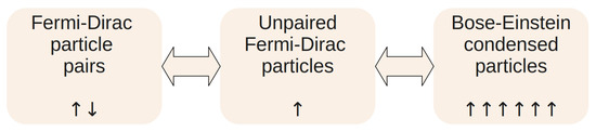
Figure 1.
The proposed thermodynamic model. The equilibrium transitions among the three particle populations are illustrated by the block arrows. The vertical arrows illustrate spin correlations.
Within a Fermi–Dirac particle pair, the spin correlation is either anti-parallel (spin-singlet state) or parallel (spin-triplet state). Generally, the spin-singlet state is energetically favored, and we find it in virtually all materials. However, some rare materials, such as K2Cr3As3, host a spin-triplet paired electron band [9]. The parallel aligned spin-triplet pairs can also directly condense into a spin-aligned Bose–Einstein condensate; the scientific literature refers to such a condensate as a “spin-triplet superconductor”. Our methodology applies essentially in the same way for the condensation of either unpaired particles or spin-triplet pairs.
In the following, the Bose–Einstein condensation temperature is calculated according to the above-outlined concepts. These calculations are based on well-known methods of statistical physics. While preceding Bose–Einstein condensation calculations lead to divergence in the two-dimensional case, our methodology is applicable to both three-dimensional and two-dimensional scenarios, as well as the anisotropic case that lies in between these two topologies.
The practical applicability of our novel Bose–Einstein condensation model can be assessed in the context of superconductivity, where vast sets of measurements and studies have been accumulated over the past 100 years. One model assessment approach, that is well suited to large datasets, is to use AI to generate a quantitative comparison table between the model presented in this work and the BCS model of superconductivity. Upon such query, ChatGPT generated the score-board shown in Table 1, demonstrating the significant progress achieved by our present work.

Table 1.
A superconductivity-oriented comparison between the Bose–Einstein condensation model presented in this work and the BCS model, according to ChatGPT. The scoring is from 1 (worst) to 5 (best).
2. Quantum Mechanical Standing Waves of Enclosed Particles
The quantum mechanical states of enclosed particles are standing waves, located in a square potential well that is defined by the enclosure. The particle wavefunctions reflect back from the enclosure boundary. This work considers systems where the interaction among particles is negligible. Quantum mechanical standing waves are then simple harmonic waves. Enclosed particle examples where a non-interacting model applies at low temperatures: noble gases, or delocalized electrons within the interior of a metal. In the delocalized electron case, their electrostatic potential is counter-balanced by the positively charged lattice nuclei. (Note: when the interaction among particles is non-negligible, the allowed quantum mechanical states are solutions of the Gross–Pitaevskii equation. This equation incorporates interactions among particles through a pseudopotential, and its non-linearity arises from these interactions. The density of states formula then becomes more complex than Equations (8) and (9). The rest of the article applies in the same way, but the appropriate density of state formulation must be used. In the context of superconductivity, the Gross–Pitaevskii equation has been shown to be relevant for sub-micron-sized mesoscopic superconductors, whose size is comparable to the superconducting coherence length [10]).
Consider a cube-shaped enclosure with dimensions , , and . A standing wave’s wavenumbers may take on the values illustrated in Figure 2; specifically the following:
where .
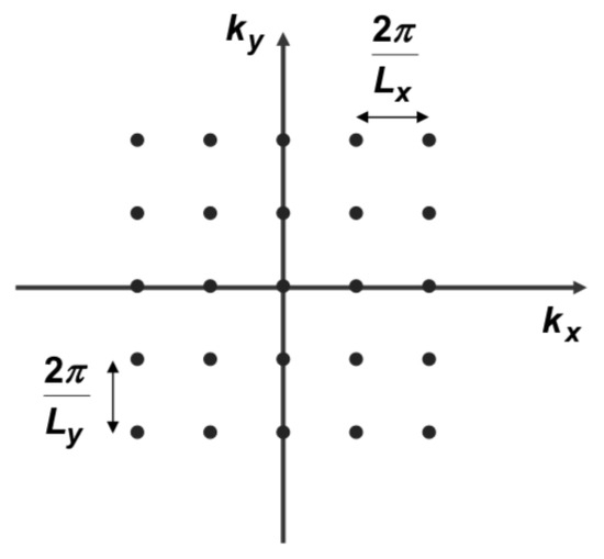
Figure 2.
A k-space representation of delocalized electron states.
When the particle movement is restricted to a 2-dimensional plane, the allowed wavenumbers are
with .
Each gridpoint of Figure 2 represents an allowed state. In the k-space of Figure 2, there is only one state per every volume element. Thus, the k-space density of allowed states is
Similarly, the k-space density of 2-dimensional states is
The kinetic energy of any given state is
where for the 3-dimensional case and for the 2-dimensional case.
We want to determine the number of delocalized particle states that are within a threshold wavenumber. In the k-space representation, these states occupy a Fermi-sphere, with radius . The number of delocalized states within radius is
We denote the total density of particles by . The relationship between the particle density and is
In the case of a 2-dimensional plane, delocalized particles occupy a Fermi-disc, with radius . We use the symbol to refer to the areal density, as it is dimensionally different from the volumetric density. The relationship between and becomes
The energy of particles at is called the Fermi energy:
Now, we calculate the density of energy eigenstates as a function of particle energy. Using Equation (3), we obtain and the following expression for :
The density of three-dimensional particle states grows with the square root of particle energy.
An analogous calculation of yields
The above equation means that the density of particle states is constant in the two-dimensional case.
3. The Entropy of a Delocalized Configuration
Suppose that we have N indistinguishable particles that are arranged among M available states. In this context, indistinguishability means that the exchange of any two particles does not impact any thermodynamic property, such as the number of available states or the energy levels of these states. How many configurations are available for distribution? Distributing into M states is analogous to putting each particle into one of M boxes in a row; these boxes have walls between them. Essentially, we have a row of N particles and walls, and we want to count their possible configurations. We count up to elements, and each consecutive element can be either a particle type or a wall type.
The number of configurations is
The entropy S of a particle configuration is defined as
where is the Boltzmann constant, and W is the number of available configurations.
According to Equation (3), an electron’s energy depends on the absolute value of its wavenumber k. However, each k state can be realized through various combinations of , , and wavenumbers; these possibilities are denoted by the available states.
Let be the number of particles with wavenumber k. In terms of thermodynamics, all particles are indistinguishable; each one has the exact same kinetic energy. The number of configurations for all particles is given by
We use Stirling’s approximation for calculating the logarithms:
which converges for large n. The total entropy then becomes
where we used the approximation. Differentiating S with respect to a selected variable yields
The total kinetic energy is
where is calculated from Equation (3), and U remains constant for a closed system. In thermal equilibrium, the particles distribute themselves such that the total entropy is maximized. For a given number of particles, any variation around thermal equilibrium keeps the total number of particles constant:
Therefore, in order to find the thermodynamically favored equilibrium configuration, we must maximize S under the constraints of fixed U and N. This implies for each the following condition:
where and have been defined as optimization constants. For an adiabatic process, the above differential becomes , which implies that is in fact the chemical potential. Since a potential is defined with respect to a reference, to calculate we must know where the new particles are added from. Evaluating the above differentials yields
We solve the above equation for :
The average occupancy number of states with energy is
The above formula is known as the Bose–Einstein distribution. We are interested in finding the thermodynamic conditions that allow for the coherent Bose–Einstein condensation of particles, with the distribution given by Equation (19).
We now evaluate the parameter. When the number of particles is allowed to vary, the change in entropy is calculated using Equation (16):
At the same time, is also given by the first law of thermodynamics:
where T is temperature, P is pressure, and is the chemical potential. Since there is no volume change within a fixed enclosure, the above equation leads to the following formulation of the entropy change:
4. The Continuum Limit of Large Distributions
Using (19), the total number of particles is
Recalling the density of k-space elements given by Equation (1), in the continuum limit, one may replace the summation by integrating over all possible wavenumbers:
which gives the following particle density:
Replacing the wavenumber integration by integrating over particle energy values, we obtain the following expression for the density of delocalized particles for the 3-dimensional and 2-dimensional cases, respectively:
where the parameter of Equation (8) gives the density of particle states at a given energy.
Let us consider the role of chemical potential . In our context, the Fermi sea is the source of electrons during a change in their total number. If a stable Fermi sea and Bose–Einstein condensate co-exist, the condition represents their balance. (Note: the condition means that energy is gained by a particle moving from the Fermi sea to tha Bose–Einstein condensate, or vice versa. Therefore, under the condition, a thermodynamic balance between a Fermi sea and Bose–Einstein condensate would require an electrostatic potential difference to counter-balance the chemical potential difference. Within any given material, the Fermi sea and Bose–Einstein condensate occupy the same region; i.e., there cannot be any electrostatic potential difference between them. This leads to the conclusion that the condition is a pre-requisite for the co-existing Fermi sea and Bose–Einstein condensate being in thermodynamic balance within any given material.)
Considering the finite number of available particles, the density of Bose–Einstein-condensed particles can be summarized by the following two rules:
- If Equation (24) can be solved in the case, the spin-triplet Fermi sea particles flow into the Bose–Einstein condensate till the condition is established; the Fermi sea and Bose–Einstein condensate co-exist at the given temperature.
- If Equation (24) cannot be solved for , all spin-triplet Fermi sea particles flow into the Bose–Einstein condensate when it becomes thermodynamically favorable. A thermodynamic precondition is that the pre-condensation mean energy in the Dirac–Fermi sea must be at least as high as the mean energy of the Bose–Einstein condensate.
If the condition can be fulfilled, we arrive at the following expression for the density of particles:
In the above expression, the term diverges at the energy value. This divergence expresses that having an infinite reservoir of Fermi sea particles pulls an infinite number of them into the Bose–Einstein ground state. It is exactly the dynamics that characterizes Bose–Einstein condensates: particles are continuously condensed into the ground state as long as there is an available supply. Despite this ground state divergence, as we shall see below, the overall integral still converges to a finite value.
5. Bose–Einstein Condensation
The phase transition that we derive in this section is unique in the sense that it is driven by delocalized wavefunction interactions, and not by local interactions between nearby particles. In the following, we calculate Bose–Einstein condensation dynamics for three topological scenarios.
5.1. Three-Dimensional Isotropic Case
This scenario is relevant for non-interacting gases. Also, elementary metal-based superconductors fall into this category, as evidenced by their isotropic diamagnetism.
Let us re-write Equation (25) in terms of the dimensionless variable:
To evaluate the above integral, we use the Maclaurin series expansion of :
For each a value, we evaluate the integral expression by making the variable change:
where is the so-called gamma function, with . Substituting the above result into Equation (26), we obtain
In the above equation, the summation result is given by the Riemann zeta function:
Equation (27) expresses the relationship between the Bose–Einstein-condensed particle density and temperature. As we obtained Equation (27) for the case of , the temperature appearing in this equation is in fact the limiting temperature of Bose–Einstein condensation that allows for a co-existence between the Fermi sea and Bose–Einstein condensate particle states:
where the density of Bose–Einstein-condensed particles appears abruptly at the phase-change temperature, i.e., = 0 for .
Finally, we rearrange the above equation to solve for :
Equation (29) is an important result: it defines the limiting temperature of an isotropic Bose–Einstein condensation. This equation has been known in the scientific literature; it was first derived by Fritz London in 1938 [1], and is nowadays further explained in textbooks [11]. However, Equation (29) was previously derived by assuming the Bose–Einstein condensation of all available particles, and without investigating the chemical potential’s role. Here, we see that fulfilling the condition means that the Fermi–Dirac and Bose–Einstein particle populations co-exist at any temperature. Only in the limit do all Fermi–Dirac particles undergo Bose–Einstein condensation.
Let us denote by and the density of spin-singlet and unpaired Fermi–Dirac particles, evaluated just before the Bose–Einstein condensation. As it is the unpaired particles that are capable of Bose–Einstein condensing, it follows that .
In elementary metals, is a tiny fraction of the total density of delocalized electrons. Let us consider lead, as a representative elementary metal superconductor. Based on lead crystal’s 0.5 nm unit cell dimension and the +2 valence state of lead sites, we estimate n = (0.4 nm)−3 total delocalized electron density in lead metal. Applying = 7.2 K of lead metal to Equation (28), we obtain that is only 0.05%. Lead material has = 52 nm magnetic field penetration depth and effective electron mass; we can use the London equation, which was derived in [8], to find the density of superconducting electrons at . Carrying out this calculation yields = (0.37 nm)−3 superconducting electron density. These data imply and in elementary metals. Determining thus becomes the basis for estimating in isotropic materials.
In hydrated or deuterated metals, the ratio can reach an order of magnitude that is higher in value than in elementary metals, even at ambient pressure. The authors of [12] achieved 60 K ambient pressure superconductivity in rapidly cooled deuterated palladium (PdD); this is the highest superconducting temperature achieved so far in a binary isotropic material. The electronic structure of hydrated palladium has been extensively studied, and these studies conclude that the palladium–hydrogen bond mainly has a covalent character. The +2 valence of metallic palladium therefore turns into approximately +1 valence in PdD. Based on PdD crystal’s 0.414 nm unit cell dimension and +1 valence, we estimate n = (0.414 nm)−3 total delocalized electron density. Applying = 60 K of PdD metal to Equation (28), we obtain that is 0.5% in PdD. The different Fermi–Dirac unpairing process in elementary versus hydrated metals is illustrated by their opposite nuclear mass dependence: heavier lead isotopes yield lower , while heavier hydrogen isotopes yield higher in hydrated palladium. Specifically, the authors of [12] achieved 60 K superconductivity with PdD, but only 54 K superconductivity with PdH. The involved catalytic processes shall be examined in Section 6.
The Buckminsterfullerene-based Rb3C60 material is an example of even higher fraction. It comprises 1.45 nm spacing between the +1 valence Rb sites; and thus, we estimate n = (1.45 nm)−3 total delocalized electron density. Applying = 29 K of Rb3C60 metal to Equation (28), we obtain that is 3% in Rb3C60. Table 2 summarizes the two-orders-of-magnitude variation across these reviewed materials. Such large variation in the ratio demonstrates the existence of catalytic processes that determine the rate of unpaired electron production within the Fermi–Dirac sea.
Table 2.
The fraction of delocalized electrons that undergo Bose–Einstein condensation at isotropic materials’ superconducting transition temperature.
Let us briefly consider those metals that do not superconduct at any temperature. The interference of internal magnetic fields explains the absence of superconductivity in ferromagnetic materials: an analogous effect has been observed in superfluids as well. Iron, for example, becomes superconducting only above the pressure where its crystal structure changes into a non-ferromagnetic phase.
We derived Equation (29) for the case, and the next step is to understand what happens in the case. We discussed in Section 4 that the term diverges at the energy value, which means that a significant fraction of electrons condenses into the quantum mechanical ground state. Therefore, in the case, we must treat those electrons that occupy the ground state separately. We therefore formulate Equation (23) as follows, keeping in mind the condition:
In the continuum limit, the corresponding electron density becomes
Dividing by and substituting Equation (29), we obtain
Equation (32) defines the ratio of Bose–Einstein-condensed electrons that occupy the quantum mechanical ground state, and it is graphically illustrated in Figure 3. It can be seen that nearly all Bose–Einstein-condensed electrons occupy the ground state at . The percentage of Bose–Einstein-condensed electrons that occupy the ground state gradually reduces to zero in the temperature limit. This result explains the experimental observation of in all superconducting materials; the London equation tells us that the infinite value corresponds to the zero density of electrons in the superconducting ground state at temperature, exactly as predicted by Equation (32).
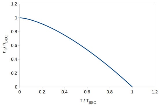
Figure 3.
The ratio of Bose–Einstein-condensed electrons that occupy the ground state in isotropic electron condensates, as a function of .
5.2. Stacked 2-Dimensional Case
In this section, we describe Bose–Einstein condensation for the purely 2-dimensional case. Let us firstly calculate the 2-dimensional case for , starting from the 2-dimensional analogue of Equation (25):
where the parameter of Equation (9) gives the density of electron states at a given energy.
As before, we re-write this equation in terms of the dimensionless variable:
To evaluate the above integral, we again use the identity. For each a value, the integral expression yields
The integral expression of Equation (34) thereby evaluates to
The above summation diverges as the Riemann zeta function grows to infinity in the limit. The divergence of means that the density of Bose–Einstein condensate grows as long as there is a supply of electrons, i.e., there is no thermodynamically favorable co-existence between a 2-dimensional Bose–Einstein condensate and Fermi–Dirac sea. The 2-dimensional case is therefore simpler than the 3-dimensional one: if Bose–Einstein condensation becomes thermodynamically favored, all delocalized electrons undergo Bose–Einstein condensation via the mediation of unpaired electrons, implying already at the superconducting transition temperature.
We calculate from the thermodynamic precondition that the pre-condensation mean energy in the Dirac–Fermi sea must be at least as high as the mean energy of the Bose–Einstein condensate. At any given temperature, the Bose–Einstein condensate’s mean energy is .
There are two electrons per energy eigenstate in the Dirac–Fermi sea. Recalling from Equation (9) that the energy eigenstates are evenly spaced in a 2-dimensional metal, the mean energy of the Dirac–Fermi sea is of its Fermi energy level. It follows that is given by the following formula:
We rearrange the above equation to solve for :
Equation (36) implies a linear relationship. Regarding experiments, nearly 2-dimensional Bose–Einstein condensation has been studied in the context of thin superfluid films [13]. As shown in Figure 4, the anticipated approximate relationship is indeed experimentally observed.
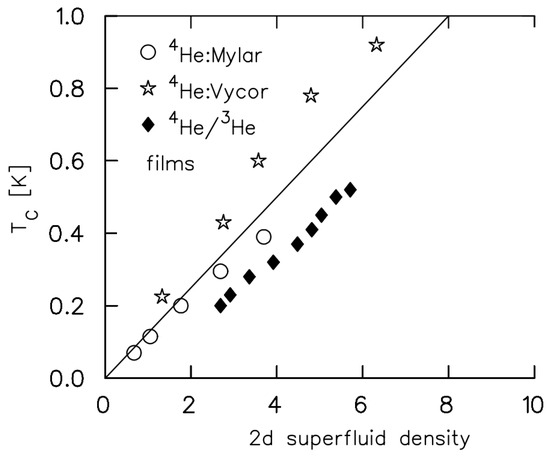
Figure 4.
The relationship in nearly 2-dimensional superfluids, reproduced from [13].
While a purely 2-dimensional case may be a mathematical abstraction, strongly anisotropic materials approach this limit, and Equation (36) becomes a good approximation for strongly anisotropic materials.
5.3. Generalized Anisotropic Case
Next, we consider a generalized case in-between the 3-dimensional isotropic and the stacked 2-dimensional topologies. In the context of superconductors, the anisotropic topology means that conduction band electrons have 3-dimensional delocalization, but their superconducting diamagnetism has significant anisotropy. Practically all high-temperature superconductors fall into this category. We model this class of materials by interpolating between the 3-dimensional and 2-dimensional topologies.
When the particle states are not purely 2-dimensional, a solution for = 0 shall exist. Revisiting Equation (34), we firstly carry on with the 2-dimensional calculation, using the symbolic notation.
Let denote the inter-layer spacing between the crystal planes that more strongly conduct electrons. In order to compare 3-dimensional versus 2-dimensional results using dimensionally matching equations, we shall use the density notation for the 2-dimensional computation. Using Equation (34), we can now express the Bose–Einstein-condensed electron density in terms of its limiting temperature:
We rearrange the above equation to solve for :
For the generalized anisotropic case, the dimensionality of electron conduction is somewhere between 2-dimensional and 3-dimensional. By comparing Equation (38) against (29), it is possible to formulate the generalized formula, and there is only one dimensionally correct method of carrying this out. Specifically, the term is the generalization of the 3-dimensional and 2-dimensional terms. The factor remains the same for any topology. In order for the formula to yield temperature and to match with the generalized particle density definition, the term must be present as well. I.e., the dimensionally generalized particle density is , where is the 3-dimensional particle density and is the inter-layer distance of the crystal structure. The anisotropic formula becomes:
where D is the dimensionality parameter. is well-defined in the range, and isotropic materials have the value. Experimentally, the value of D can be inferred via London penetration depth measurements along the various axes of the crystal structure. As before, it follows from the condition that the Fermi–Dirac and Bose–Einstein-condensed phases co-exist at any temperature.
6. Discussion
6.1. The Role of Unpaired Fermi–Dirac Electrons in Superconductors
The density of unpaired delocalized electrons can be measured via the NMR Knight shift, which they produce. High-temperature superconductors’ Knight shift value starts dropping exactly below their superconducting transition point. This phenomenon is illustrated in Figure 5, taking the example of a cuprate-type superconductor. In the case of optimally doped , its Knight shift remains constant as the temperature is lowered towards , and then starts sharply decreasing in the region. In the case of underdoped , this phenomenon is much weaker, but still observable under variable applied magnetic field: the Knight shift remains constant as the magnetic field strength is lowered towards the critical magnetic field strength , and then starts decreasing in the region. Analogous Knight shift charts are observed for other high-temperature superconductors as well. Figure 6 shows the example of an iron-based superconductor. This experimental phenomenon directly supports our mathematical model.
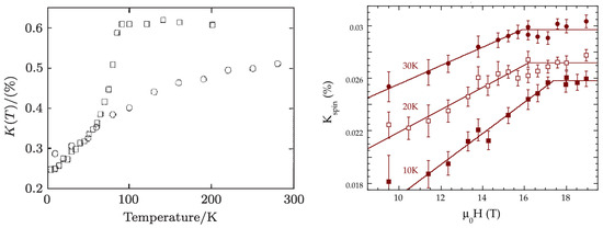
Figure 5.
The signature of unpaired electron condensation is the Knight shift value drop in , upon transition into superconducting state. Left: The Knight shift versus temperature, reproduced from [14]. The square symbols represent optimally doped with = 90 K, the round symbols represent underdoped . Right: The Knight shift versus magnetic field strength for underdoped , reproduced from [15]. The measurements were made at the various indicated temperatures; the Knight shift drop starts at for the given temperature.
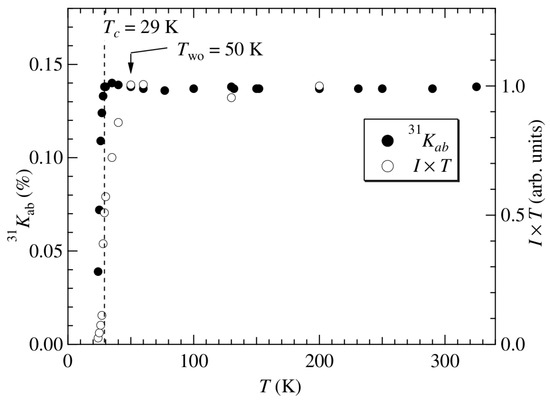
Figure 6.
The signature of unpaired electron condensation is the Knight shift value drop in , upon transition into superconducting state. The Knight shift was measured by 31P NMR method. Reproduced from [16].
Incoherent electrons’ pairwise spin correlation, which forms spontaneously, is thermodynamically favored over the single-electron occupancy of an energy eigenstate. That is why only a small fraction of delocalized electrons contribute to the Knight shift effect, which is shown in Figure 5 and Figure 6.
6.2. The Catalysis of Fermi–Dirac Electrons’ Unpairing
It is seen in Table 2 that is generally a tiny fraction of the total delocalized electron density, i.e., only a small fraction of Fermi–Dirac electrons is unpaired. To predict materials with higher , one pre-requisite is to identify the catalytic effects that induce electron unpairing.
The PdD example of Table 2 demonstrates that the density of unpaired electrons increases with temperature in materials such as PdD. Rapid cooling then allows such materials to become superconducting at higher-than-usual temperature. A logical prediction is that the superconducting transition temperature of such materials can be further increased by firstly heating them, and then rapidly cooling.
Let us now review the effect of phonons, which were traditionally thought to play a key role in superconductivity. Table 3 lists the highest elementary metals at ambient pressure. Elementary metals in the > 2 K group are either single-isotope elements or display the isotope effect, where M is the isotope mass. It is therefore probable that all metals of the > 2 K group would display the isotope effect, if various isotopes of each element were available. The isotope effect is associated with phonon interactions for two reasons: (i) the Debye frequency of phonons is also proportional to , and (ii) except for electron–phonon interactions, the nuclear mass plays no role in delocalized electron dynamics.
Table 3.
The listing of highest elementary metals at ambient pressure. The last column shows the isotope effect measurement, if the given element has various isotopes.
In contrast, for elementary metals in the < 2 K group, the isotope mass has a randomly varying coefficient and there is no isotope effect at all in metals such as Ru or Zr. This data demonstrates that phonons play no essential role in elementary metals’ superconductivity in the < 2 K group.
These observations indicate that phonons have a mildly catalytic effect on the formation of unpaired Fermi–Dirac electrons. Without this phonon effect, elementary metals cannot reach even 2 K superconductivity at ambient pressure.
The phenomenology of catalytic phonon effects is described in reference [17], quantifying the impact of electron–phonon coupling. The experimental data reviewed in reference [17] show that in alloys, a of around 20 K can be achieved via phonon-catalyzed superconductivity.
Recently, it has been discovered that the superconductivity of K3C60 can be transiently extended even up to room temperature via the application of 10 THz electromagnetic pulses [18]. According to the authors of [18], this 10 THz excitation frequency matches a radial phonon-frequency of the C60 structure, i.e., sufficiently strong phonon oscillations unpair a significant fraction of delocalized Fermi–Dirac electrons. These results resolve a long-standing misunderstanding concerning phonons’ role in superconductivity.
6.3. Isotropic Superconductors
Equation (29) implies scaling for a given isotropic material, with all else being equal. This isotropic superconductor case is nicely illustrated by a boron-doped diamond; it is a binary-structured superconductor, where the density of conduction band electrons is proportional to the boron doping density. As illustrated in Figure 7, the of boron-doped diamond follows the anticipated relationship.
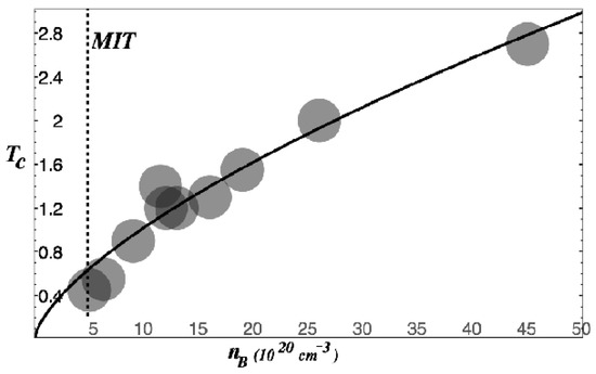
Figure 7.
The (K) of boron-doped diamond, as a function of boron concentration. The data are taken from [19]; disc sizes correspond to the error bars. The solid line represents scaling. The dashed line indicates metal–insulator transition.
6.4. Superconductors Comprising Stacked 2-Dimensional Topology
6.4.1. Optimally Doped Superconductors
Nearly all high-temperature superconductors comprise stacked conducting planes, and their delocalized electron concentration is defined by the doping concentration. Their nearly 2-dimensional anisotropy can be characterized by the magnetic field penetration depth’s anisotropy. We firstly consider “optimally doped” superconductors, where is maximized. In optimally doped cuprate materials, which represent the most studied class of high-temperature superconductors, is 10–30 times larger in the perpendicular direction to the CuO2 planes than in parallel direction with respect to the CuO2 planes. These cuprate materials can therefore be characterized as strongly 2-dimensional materials, in which superconducting electrons move mainly along the CuO2 planes. We thus anticipate to be given by Equation (36).
In a remarkable work, the authors of [20] demonstrate a rather precise relationship for high-temperature superconductors, where x is the spacing between the doping sites that donate delocalized electrons, N is the number of CuO2 planes within the unit cell, and m2K is a phenomenologically determined constant. This relationship is known as the Roeser–Huber formula, and it is illustrated in Figure 8. Despite the Roeser–Huber formula’s accuracy, so far, it gained little attention among superconductivity researchers because it does not match with preceding superconductivity theories.
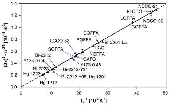
Figure 8.
The Roeser–Huber relationship in iron-based and cuprate-based high-temperature superconductors, reproduced from [13].
Comparing the Roeser–Huber formula against Equation (36), one finds and . In most cuprate superconductors, one finds N = 3, and occasionally N = 2 or N = 4. The dimensionless parameter thus usually evaluates to 2, i.e., , and it is clearly seen that the Roeser–Huber formula is in fact Equation (36). The match between Equation (36) and experimental data is therefore remarkable, and validates our theory.
6.4.2. Underdoped Superconductors
The underdoped regime of high-temperature superconductors is characterized by a gradually growing delocalized electron concentration, as a function of the doping parameter. The concentration of delocalized electrons is approximately zero near the insulator–metal transition point, and gradually grows with increasing doping levels. Equation (36) indicates that the concentration of delocalized electrons must be the limiting factor in this regime.
Around 1990, Y. Uemura found the relationship, which universally holds for the underdoped regime of cuprate superconductors and was considered highly unexpected by the superconductivity theories that existed at the time of its discovery. This relation is shown in Figure 9. The data of Figure 9 were obtained via muon spin relaxation measurement, where the muon spin relaxation rate is proportional to . The London equation relates the measurements to the superconducting electron density. For nearly 2-dimensional materials, we can express the superconducting electron density using the previously discussed formula, where is the areal density of Bose–Einstein-condensed electrons, and is the inter-layer distance of superconducting planes. At , the Bose–Einstein-condensed electrons all occupy the ground state, thus contributing to the superconducting current. Therefore, the observation leads to the relationship as long as and remain constant. The obtained relationship matches with Equation (36), i.e., we observe that Uemura’s linear relationship is a second validation of Equation (36).
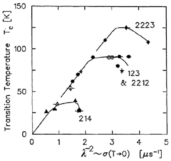
Figure 9.
The relationship, which is universally valid in the underdoped region of cuprates. The labels indicate various cuprate materials. Reproduced from [21].
At the optimal doping point, deviates from the linear Uemura relationship observed in the underdoped regime, implying that or become significantly impacted by the doping concentration. On the other hand, the Roeser–Huber formula is valid at the optimal doping point. From this point of view, the Uemura and Roeser–Huber relationships can be seen as complementary.
6.4.3. Overdoped Superconductors
While the synthesis of optimally doped superconductors is relatively straightforward, further increases of doping concentration are experimentally more difficult to achieve. The synthesis of overdoped superconductors generally require harsh oxidation methods, such as ozone or fluorine treatment.
For cuprate-type superconductors, the highest is generally observed near a doping concentration, where p measures the excess charge density with respect to the Cu concentration. The p > 0.15 regime is the “overdoped region”; it is characterized by gradually descending to zero, and superconductivity completely disappears around 0.25. The corresponding superconducting phase diagram is illustrated in Figure 10. Between 1990 and 2020, this phase diagram was thought to be universally valid for cuprate-type superconductors. An analogous phase diagram was identified for iron-based superconductors as well.
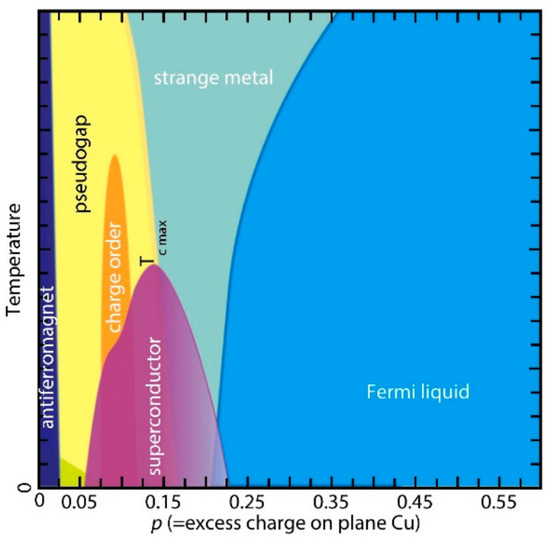
Figure 10.
The historically formulated phase diagram of cuprate superconductors, which remained unchallenged till recent years. The superconducting phase is represented by the purple dome. The yellow area represents the so-called pseudogap phase, characterized by a reduced dimensionality of delocalized electron flows. The blue area represents the usual Fermi sea.
Preceding high-temperature superconductivity theories were formulated around rationalizing the emergence of high-temperature superconductivity from a non-Fermi liquid ground state, motivated by the separation of these regions in the phase diagram of Figure 10.
Through ingenious experiments, the authors of [22,23] demonstrate that the gradual disappearance of superconductivity in the overdoped regime is just the side-effect of a growing number of crystal defects, caused by the harsh oxidation conditions. Remarkably, the authors of [22,23] developed a “high pressure oxidation” method, suitable for the defect-free synthesis of overdoped cuprates. These works show that a value of 90 K can be obtained even in the p > 0.6 region.
The results of [22,23] thus invalidate preceding high-temperature superconductivity theories by demonstrating that high-temperature superconductivity emerges from an ordinary Fermi sea ground state. On the other hand, this result is well aligned with our model of electron Bose–Einstein condensation from ordinary Fermi sea ground state.
In Section 5.3, we described the co-existence between Bose–Einstein-condensed and Fermi sea electron populations in the anisotropic case; such co-existence is indeed experimentally demonstrated in [23] for a highly overdoped superconductor. Our novel methodology is therefore suitable for the analysis of high-temperature superconductors such as Ba2CuO3.2, which are described as anisotropic rather than 2-dimensional [22].
6.5. Thin-Film 2-Dimensional Superconductors
As explained in Section 5.2, the temperature of stacked 2-dimensional superconductors depends on the pre-condensation Fermi energy level. With all else being equal, a lower Fermi energy level implies a proportionally lower value.
As the thickness of a metal film reaches below the 100 nm range, the metal–substrate interface begins impacting the Fermi energy value. In other words, the Fermi energy level becomes dependent on the substrate material.
We consider the high-temperature superconductor material that comprises stacked 2-dimensional planes. As shown in Figure 11, experimental measurements on a thin superconductor film indeed shows that becomes dependent on the substrate material as the film thickness reaches below the 100 nm range. This effect demonstrates the predicted dependence on the pre-condensation Fermi energy level.
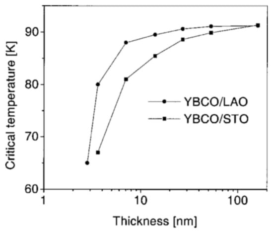
Figure 11.
The of nano-films, measured with two different substrate materials. Reproduced from [24].
6.6. Fermi Level Depletion in the Superconducting State
Our model predicts a gradual Fermi energy level depletion in superconductors as their temperature is lowered towards zero; this depletion is caused by the high electron occupancy of a Bose–Einstein condensate’s energy eigenstates.
A direct signature of this anticipated Fermi level change is reported in references [25,26,27]: these works measure , , and materials’ Fermi level relative to a silver contact. As shown in Figure 12, the Fermi level depletion upon entering superconducting state manifests as a polarity change in the superconductor–silver interface. The interface polarity was detected by the laser illumination technique, and the same effect was found for all superconducting materials.
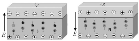
Figure 12.
Fermi level depletion upon transition from normal to superconducting state, manifesting as interface polarity change. Left: Ag–superconductor interface in superconducting (S) state. Right: Ag–superconductor interface in normal (N) state. The polarity is measured by laser-induced production of electron–hole pairs, which create photovoltaic effect.
In contrast, preceding superconductivity theories consider superconducting electrons to remain in the Fermi sea, i.e., they predict no Fermi level change upon superconducting state transition, and thus become contradicted by experiments.
6.7. Bose–Einstein Condensation from Spin-Triplet Paired Electron State
K2Cr3As3 is an exemplary material that is thought to contain an electron band comprising delocalized electrons with parallel spin correlation [9]. Such electron pairs are also being referred to as a “spin-triplet” state.
The existence of a spin-triplet comprising a Fermi–Dirac sea contradicts the historically formulated electron statistics postulates. On the other hand, a spin-triplet comprising Fermi–Dirac sea is perfectly compatible with the results of reference [8], which proves the pairwise Pauli exclusion limit of incoherent electron states, regardless of their parallel or anti-parallel spin correlation.
Electronic structure studies on K2Cr3As3 show that it comprises three distinct delocalized electron bands: two are nearly 1-dimensional, and one is nearly isotropic [9,28]. Superconductivity is associated with the phase transition of the isotropic electron band, and this nearly isotropic band is thought to host spin-triplet electron pairs.
Despite its relatively low superconducting temperature of = 6.2 K, K2Cr3As3 maintains its superconducting state even under >20 T magnetic field at temperature. While lead metal has a similar superconducting temperature of = 7.2 K, lead looses its superconductivity already under a 0.08 T magnetic field at the same temperature. Because of these properties, K2Cr3As3 is being classified as an “unconventional” superconductor.
Considering that the superconductivity-related topology is nearly isotropic in K2Cr3As3, we compare its experimental data against the equations of Section 5.1. Its superconducting electron density can be characterized by magnetic field penetration depth measurements. As shown in Figure 13, the experimental superconducting electron density data closely match Equation (32).
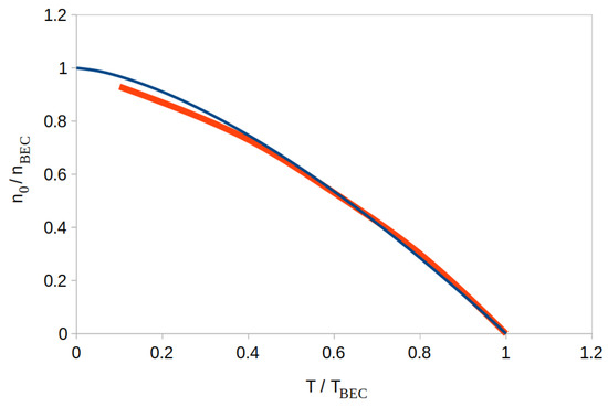
Figure 13.
The ratio as a function of in K2Cr3As3. The red curve is the experimental data from [28], and the blue curve corresponds to Equation (32).
The matching data of Figure 13 in fact requires that remain constant across the charted temperature range. This implies that all (or most) spin-triplet state electrons Bose–Einstein condense at the transition temperature.
7. Conclusions
We calculated the Bose–Einstein condensation temperature formulas for isotropic, stacked 2-dimensional, and anisotropic topologies. A remarkable match was found between the calculated temperature formulas and experimental data. We identified the coexistence of Fermi–Dirac and Bose–Einstein-condensed particle populations in the isotropic and anisotropic cases, while the stacked 2-dimensional topology leads to a sharp phase transition.
We demonstrated that the superconducting phase transition is the Bose–Einstein condensation of unpaired delocalized electrons. Our theory applies to both conventional and high-temperature superconductors.
We anticipate that the Bose–Einstein condensation temperature formulas derived in this work may lead to a generally accepted superconductivity theory based on conduction band electrons’ Bose–Einstein condensation, and facilitate a rational search for higher-temperature superconductors.
Funding
This research was partly funded by Marc Fleury.
Data Availability Statement
No new data were created in this study; data sharing is therefore not applicable.
Acknowledgments
The author thanks Giorgio Vassallo for insightful discussions.
Conflicts of Interest
The author declares no conflicts of interest.
References
- London, F. On the Bose–Einstein Condensation. Phys. Rev. 1938, 54, 947–952. [Google Scholar] [CrossRef]
- The Nobel Prize in Physics 2001. Available online: https://www.nobelprize.org/prizes/physics/2001/popular-information/ (accessed on 20 July 2025).
- Villarreal, C.; de Llano, M. Bose-Einstein condensation in quasi-2D systems: Applications to high-Tc superconductivity. In Quantum Field Theory under the Influence of External Conditions; World Scientific: Singapore, 2010. [Google Scholar]
- Harrison, N.; Chan, M.K. Magic gap ratio for optimally robust fermionic condensation and its implications for high-Tc superconductivity. Phys. Rev. Lett. 2022, 129, 017001. [Google Scholar] [CrossRef] [PubMed]
- Schneider, T.; Pedersen, M.H. Cuprate Superconductors: Universal Properties and Trends, Evidence for Bose-Einstein Condensation. J. Supercond. 1994, 7, 593–598. [Google Scholar] [CrossRef]
- Yang, J.; Luo, J.; Yi, C.; Shi, Y.; Zhou, Y.; Zheng, G.Q. Spin-triplet superconductivity in K2Cr3As3. Sci. Adv. 2021, 7, eabl4432. [Google Scholar] [CrossRef] [PubMed]
- Nakamura, J.; Liang, S.; Gardner, G.C.; Manfra, M.J. Direct observation of anyonic braiding statistics. Nat. Phys. 2020, 16, 931–936. [Google Scholar] [CrossRef]
- Kovacs, A.; Vassallo, G. Rethinking Electron Statistics Rules. Symmetry 2024, 16, 1185. [Google Scholar] [CrossRef]
- Ogawa, S.; Miyoshi, T.; Matano, K.; Kawasaki, S.; Inada, Y.; Zheng, G.Q. Single Crystal Growth of and Hyperfine Couplings in the Spin-Triplet Superconductor K2Cr3As3. J. Phys. Soc. Jpn. 2023, 92, 064711. [Google Scholar] [CrossRef]
- Shanenko, A.A.; Tempere, J.; Brosens, F.; Devreese, J.T. Mesoscopic samples: The superconducting condensate via the Gross–Pitaevskii scenario. Solid State Commun. 2004, 131, 409–414. [Google Scholar] [CrossRef]
- Pethick, C.J.; Smith, H. Bose–Einstein Condensation in Dilute Gases; Cambridge University Press: Cambridge, UK, 2001. [Google Scholar]
- Syed, H.M.; Gould, T.J.; Webb, C.J.; Gray, E. Superconductivity in palladium hydride and deuteride at 52–61 kelvin. arXiv 2016, arXiv:1608.01774. [Google Scholar]
- Uemura, Y.J. Condensation, excitation, pairing, and superfluid density in high-Tc superconductors. J. Phys. Condens. Matter 2004, 16, S4515. [Google Scholar] [CrossRef]
- Luo, J.-L. The electronic state phase diagram of copper oxide high-temperature superconductors. In Advances in Theoretical and Experimental Research of High Temperature Cuprate Superconductivity; World Scientific: Singapore, 2020; pp. 1–26. [Google Scholar]
- Kačmarčik, J.; Vinograd, I.; Michon, B.; Rydh, A.; Demuer, A.; Zhou, R.; Mayaffre, H.; Liang, R.; Hardy, W.N.; Bonn, D.A.; et al. Unusual interplay between superconductivity and field-induced charge order in YBa2Cu3Oy. Phys. Rev. Lett. 2018, 121, 167002. [Google Scholar] [CrossRef] [PubMed]
- Itoh, Y.; Adachi, S. 31P NMR studies of an iron-based superconductor Ba0.5Sr0.5Fe2(As1−xPx)2 with Tc = 29 K. J. Phys. Conf. Ser. 2020, 1590, 012011. [Google Scholar] [CrossRef]
- Surma, M. A New Semiempirical Formula for Superconducting Transition Temperatures of Metals and Alloys. Phys. Solidi B 1983, 116, 465–474. [Google Scholar] [CrossRef]
- Rowe, E.; Yuan, B.; Buzzi, M.; Jotzu, G.; Zhu, Y.; Fechner, M.; Först, M.; Liu, B.; Pontiroli, D.; Riccò, M.; et al. Resonant enhancement of photo-induced superconductivity in K3C60. Nat. Phys. 2023, 19, 1821–1826. [Google Scholar] [CrossRef]
- Klein, T.; Achatz, P.; Kacmarcik, J.; Marcenat, C.; Gustafsson, F.; Marcus, J.; Bustarret, E.; Pernot, J.; Omnes, F.; Sernelius, B.E.; et al. Metal-insulator transition and superconductivity in boron-doped diamond. Phys. Rev. B 2007, 75, 165313. [Google Scholar] [CrossRef]
- Roeser, H.P.; Haslam, D.T.; Lopez, J.S.; Stepper, M.; Von Schoenermark, M.F.; Huber, F.M.; Nikoghosyan, A.S. Electronic Energy Levels in High-Temperature Superconductors. J. Supercond. Nov. Magn. 2011, 24, 1443–1451. [Google Scholar] [CrossRef]
- Keller, H. Positive muons as probes in high-Tc superconductors. In Exotic Atoms in Condensed Matter; Springer: Berlin/Heidelberg, Germany, 1992. [Google Scholar]
- Sederholm, L.; Conradson, S.D.; Geballe, T.H.; Jin, C.Q.; Gauzzi, A.; Gilioli, E.; Karppinen, M.; Baldinozzi, G. Extremely overdoped superconducting cuprates via high pressure oxygenation methods. Condens. Matter 2021, 6, 50. [Google Scholar] [CrossRef]
- Gauzzi, A.; Klein, Y.; Nisula, M.; Karppinen, M.; Biswas, P.K.; Saadaoui, H.; Morenzoni, E.; Manuel, P.; Khalyavin, D.; Marezio, M.; et al. Bulk superconductivity at 84 K in the strongly overdoped regime of cuprates. Phys. Rev. B 2016, 94, 180509. [Google Scholar] [CrossRef]
- Zhai, H.Y.; Chu, W.K. Effect of interfacial strain on critical temperature of YBaCu3O7−δ thin films. Appl. Phys. Lett. 2000, 76, 3469–3471. [Google Scholar] [CrossRef]
- Chu, Z.; Chang, F.G.; Liu, Z.Y.; Han, L. Photovoltaic effect in Ag/MgB2 heterostructure. J. Alloys Compd. 2019, 793, 662–671. [Google Scholar] [CrossRef]
- Chu, Z.; Ma, Z.P.; Yang, F.; Han, L.; Zhang, N.; Chang, F.G. Origin of photovoltaic effect in (Bi, Pb)2Sr2Ca2Cu3O10+d/Ag heterostructure. J. Alloys Compd. 2017, 724, 413–420. [Google Scholar] [CrossRef]
- Yang, F.; Liu, H.; Liu, H.; Lu, Q.; Chang, F. Polarity switching of the photo-induced voltage in YBCO/Ag heterojunction. J. Phys. Chem. Solids 2020, 138, 109232. [Google Scholar] [CrossRef]
- Watson, M.D.; Feng, Y.; Nicholson, C.W.; Monney, C.; Riley, J.M.; Iwasawa, H.; Refson, K.; Sacksteder, V.; Adroja, D.T.; Zhao, J.; et al. Multiband One-Dimensional Electronic Structure and Spectroscopic Signature of Tomonaga-Luttinger Liquid Behavior in K2Cr3As3. Phys. Rev. Lett. 2017, 118, 097002. [Google Scholar] [CrossRef] [PubMed]
Disclaimer/Publisher’s Note: The statements, opinions and data contained in all publications are solely those of the individual author(s) and contributor(s) and not of MDPI and/or the editor(s). MDPI and/or the editor(s) disclaim responsibility for any injury to people or property resulting from any ideas, methods, instructions or products referred to in the content. |
© 2025 by the author. Licensee MDPI, Basel, Switzerland. This article is an open access article distributed under the terms and conditions of the Creative Commons Attribution (CC BY) license (https://creativecommons.org/licenses/by/4.0/).