Chebyshev Collocation Solutions to Some Nonlinear and Singular Third-Order Problems Relevant to Thin-Film Flows

Abstract

This paper concerns accurate spectral collocation solutions, more precisely Chebyshev collocation (ChC), to some third-order nonlinear and singular boundary value problems on unbounded domains. The problems model some draining or coating fluid flows. We use exclusively ChC, in the form of Chebfun, avoid any obsolete shooting-type method, and provide reliable information about the convergence and accuracy of the method, including the order of Newton’s method involved in solving the nonlinear algebraic systems. As a complete novelty, we combine a graphical representation of the convergence of the Newton method with a numerical estimate of its order of convergence for a more realistic value. We treat five challenging examples, some of which have only been solved by approximate methods. The found numerical results are judged in the context of existing ones; at least from a qualitative point of view, they look reasonable.

1. Introduction

The problems considered in this paper stem from real-world thin-film flow scenarios. The oldest and perhaps the most important reference in this respect is our contribution [1]. We used the Chebyshev tau method a few years ago to study the linear stability of Marangoni-type thin-layer flows on an inclined plane (see [2]). In a previous paper [3], we dealt with conventional ChC and Chebfun solutions to some challenging second-order nonlinear and singular boundary value problems. In a recent paper [4], we successfully solved a set of challenging third-order nonlinear boundary value problems of Blasius type.

Three distinct spectral collocation methods, namely Laguerre collocation (LC), Laguerre–Gauss–Radau collocation (LGRC) and mapped Chebyshev collocation (ChC) have been used to solve some challenging systems of boundary layer type of third and second orders in our paper [5]. Due to the very poor conditioning of the Laguerre differentiation matrices, the LGRC method has proven to be inappropriate to solve some singular boundary problems.

In this paper, we continue the study of viscous flows in thin layers and show that the ChC method, in its more refined form, Chebfun, can solve boundary problems with various singularities.

Thus, this paper concerns some accurate spectral collocation solutions, more precisely Chebyshev collocation (ChC), to some third-order nonlinear and singular boundary value problems, mainly on unbounded domains. Compared to the previously quoted works, the complications now come from the introduction of boundary conditions.

Detailed proofs and derivations supporting the convergence/stability/error analysis of the general Chebyshev collocation (ChC) are available in the well-known monographs [6,7]. For the problems at hand, i.e., third-order nonlinear boundary value problems on unbounded domains, such results are far beyond the aim of this work. However, the Chebfun programming environment, which implements ChC, successfully compensates for these shortcomings. Specifically, to justify the order and convergence of Newton’s method, we provide, for the first time, a comparison between the (graphical) dynamics of Newton’s method and a numerical estimate (see (7)); they complete each other. The dynamics of the Newton method are represented in a semi-logarithmic plot of Newton’s updates versus iterations. The total error made by the ChC method is given by Formula (6), and the decrease (behavior) in the numerical coefficients of the solutions indicates the convergence of the method.

It is known that some draining or coating viscous fluid-flow problems, in which surface tension forces play an important role, can be described by a third-order ordinary differential equation of the form

$$u_{xxx}=f\left(u\right)u_x+g\left(u,\delta \right),x\in \mathbb{R}.$$

(1)

This equation—along with the boundary condition $u\to 1$ as $x\to -\infty$ (modelling a layer of fluid that is asymptotically uniform behind the draining front) and $u\to \delta$ as $x\to \infty$ where $0<\delta <<1$ (describing the draining over an already-wet surface)—is the central object of the present study. The actual form of these functions $f\left(u\right)$ and $g\left(u\right)$ varies depending on the physical context, and here we take into account some simple rational function of u (see, for example, [8]).

The solution $u\left(x,\delta \right)$ of this boundary value problem is of the greatest interest and is relevant to fluid draining problems on a dry wall involving the forces of viscosity, gravity, and surface tension, subject to a lubrication approximation (we prefer [9] for this topic). Unfortunately, this solution has some unacceptable features when u is small that are ultimately associated with the impossibility of moving a contact line $u=0$ over a non-slip dry wall.

To overcome all the difficulties in computing this solution, we will implement ChC in the form given by Chebfun. In this way, we will obtain correct information about the accuracy of the computed solution, the order of Newton’s method in solving the nonlinear algebraic system involved in Chebfun discretization, and the convergence of the solution, i.e., the behavior of the ChC coefficients of the solution. We will distinguish between the subgeometric, geometric, and algebraic convergence rates.

This approach confirms our opinion that the nonlinear and singular boundary value problems formulated on a real line can be more accurately solved by spectral collocation than by resorting to the classical shooting or other ad hoc methods.

This paper is divided naturally into two parts, although we do not formally designate it as such. In the second section, we briefly review Chebfun and comment on its applications to nonlinear and singular third-order boundary value problems. We discuss graphical and numerical methods for defining the order of convergence of the Newton method and the definition of the convergence of the ChC method. In the third section, we solve five different and challenging problems and discuss their accuracy. They came for physico-chemical hydrodynamics; we take them for granted and do not comment on their provenance. We are exclusively interested in solving them numerically.

We have chosen these problems as representative of a wide variety of others scattered throughout the literature.

Among the five problems is Landau and Levich’s famous one, which we solve without simplifying (approximating) the boundary condition at the entrance.

In an Appendix at the end of the work, a Chebfun code is provided as an example that can be easily modified to solve a wide range of bilocal problems.

2. Chebfun Solutions to a Class of Third-Order Nonlinear BVPs on the Real Line

Some physicochemical hydrodynamics problems involving surface tension forces are generally modeled by PDEs in space and time, typically containing fourth-order spatial derivatives. For instance, the thickness u of a thin viscous film flowing unsteadily on a solid surface satisfies such an equation. Whenever there is only one spatial coordinate of interest, that is, in the direction of flow, the problem can be reduced to an ODE in that variable, say $x.$ Consequently, the original fourth-order system can be explicitly integrated, taking into account the conservation of mass (see [10]). Finally, one obtains an autonomous third-order ODE of the form

$$u_{xxx}=g\left(u,\delta \right),x\in \mathbb{R}.$$

(2)

Sometimes the right-hand side contains a small physical parameter, say $\delta .$

In [11], the authors observe that the fundamental difficulty in solving such problems is connected here with the classical non-slip boundary condition, which fails to predict the advancing of the contact line of the falling film along the wall. The question of what the natural boundary condition should be at the contact line remains unsettled.

However, one way to circumvent this difficulty is to eliminate it. Thus, we will assume that the film is infinite in the sense that it extends infinitely far down the wall with a finite but small thickness. Then, the classical no-slip boundary condition can be applied at every point along the wall. This is also the meaning we will use in this work.

The equation will be solved together with two boundary conditions, one at plus infinity and the other at minus infinity.

Some results of existence and uniqueness for (2) are available, for example, in [12]. The authors use an independent variable transformation to reduce the equation to a second-order one, show the existence on a finite interval, and then apply the Arzela–Ascoli theorem.

It should be noted from the very beginning that the real axis will truncate at the finite interval $\left[-X,X\right]$, and we will observe in every situation that the results obtained are stable concerning length $X.$

2.1. ChC Implemented Using Chebfun

Chebfun is an open-source package based on Chebyshev technology. Its conception is presented, among others, in the work [13]. The book [14] is very useful in various applications of differential equations.

The philosophy behind Chebfun is to work in a solve-then-discretize mode rather than a discretize-then-solve one (see [14], p. 302).

Mathematically, we will have to solve the following boundary value problem:

$$\left\{\begin{array}{c}\mathcal{N}\left(u\left(x\right)\right)=0,x\in \mathbb{R},\\ u\to A,x\to -\infty ,\mathrm{and}u\to B,x\to \infty ,\end{array}\right.$$

(3)

where $\mathcal{N}$ is a third-order nonlinear differential operator that may possibly also depend on a parameter, and A and B are specified constants.

Chebfun searches for a solution to the problem (3) in the form

$$u_{ChC}\left(x\right):=\sum _{n=0}^{N-1}{u}_n{T}_n\left(x\right),$$

(4)

where N is a natural number and $T_n\left(x\right)$ is the usual Chebyshev polynomial of order n. It is important to observe that actually Chebfun works in the physical (values) space, i.e., it computes the nodal value of a solution in the Chebyshev–Gauss–Lobatto nodes. The connection between the nodal values of the solution and the coefficients $u_k$ of its expansion (4) is made by the Chebyshev transform.

Series, even a truncated one like (4), can converge at qualitatively different rates. It is, therefore, useful to have a precise definition of the convergence rate. This definition comes from the monograph [15], Chapter 2, and reads

$$\mathrm{if}{u}_n\sim \left\{\begin{array}{c}1/n^2,\mathrm{algebraic}\mathrm{convergence},\\ exp\left(-1.5n^{2/3}\right),\mathrm{subgeometric}\mathrm{convergence},\\ exp\left(-\mu n^r\right),\mu >0,r>0,\mathrm{geometric}\left(\mathrm{exponential}\right)\mathrm{convergence},\\ exp(-nlog\left(n\right)),\mathrm{or}\mathrm{faster}\mathrm{decay},\mathrm{super}\mathrm{geometric}\mathrm{convergence}.\end{array}\right.$$

(5)

These are all asymptotic definitions based on the behavior of series coefficients for large $n.$ They may be misleading if applied for small or moderate n. These abstract concepts become clearer with graphs, for example, on a log-linear plot of $log\left|u_n\right|$ versus n. This is what we will be performed in the following examples.

When $r=1$ in (5), the coefficients of a geometrically convergent series will be asymptotic to a straight line through the origin of the equation

$$log\left|u_n\right|=-\mu n,\mathrm{for} \mathrm{some}\mu >0.$$

Of course, strictly speaking, the problem (3) seems ill-conditioned because a boundary condition is missing. However, the absence of the independent variable x in the definition of the autonomous operator $\mathcal{N}$ implies that the origin on the $Ox$ axis can be arbitrarily specified, eliminating the need for a third boundary condition. Chebfun issues the following warning: Operator may not have the correct number of boundary conditions. Matrix is not square. The problem may be ill-posed. Despite this, Newton’s method is convergent.

As we have mentioned above, to numerically deal with this problem, we will truncate the real axis to a finite interval $\left[-X,X\right]$ for an X that is chosen arbitrarily or obtained for physical reasons. Finally, we will show that the numerical results are stable with this choice.

The domain truncation method for solving differential equations on an unbounded interval has been discussed by many authors. Our favourite reference is [16], and the works of the same author which are cited there. It is well known that if a solution $u\left(x\right)$ decays exponentially fast as $\left|x\right|\to \infty ,$ then only an exponentially small error is made by truncating the unbounded interval to $\left[-X,X\right].$ After this truncation has been performed, one may apply any numerical method in the same manner as for any problem on a bounded interval.

Because a solution to (3) is not periodic, the normal choice of spectral basis functions is Chebyshev polynomials.

It is also fully accepted, as when a non-periodic function is expanded as a Fourier series, that the coefficients decrease at an algebraic rate rather than as exponential functions of the degree $n.$

There are also the so-called mapping methods, in which an unbounded domain becomes finite. These methods can sometimes be superior to truncating the domain, especially by minimizing execution time. However, truncating the domain remains a superior method, especially with respect to ease of programming, especially with Chebfun, as well as with respect to ease of understanding.

The range for the independent variable x, the non-linear operator $\mathcal{N}$, and the boundary conditions are introduced in the Chebfun code by simple commands. A backslash command is used to solve the nonlinear algebraic system by Newton’s iterations. Some output additional information about the solution is available; thus, it enables one to track the norms of the Newton updates during the iteration and to estimate its order of convergence. The solution is a single (long) Chebfun, i.e., a polynomial of some degree. The size of the coefficients of this polynomial and how they decrease are visualized in a log-linear plot. This picture can also provide an estimation for the convergence order of the Chebyshev method (see, for instance, our paper [3]).

If we denote the Chebfun solution to the problem (3) by $u_{ChC}$, it is very valuable the estimation

$$\mathrm{norm}\left(\mathcal{N}\left(u_{ChC}\right)\right),$$

(6)

which gives us a measure of how accurately Chebfun performed. The final error estimate for the differential equations and the boundary conditions are separately provided. These error estimates are generally better than the error defined by (6).

2.2. On the Graphical and Numerical Approximation of Newton’s Convergence Order

To justify the order of convergence of Newton’s method, we provide, for the first time, a comparison between the (graphical) dynamics of Newton’s method and a numerical estimate.

Thus, when one solves the problem (3) using ChC for the involved Newton’s method, a numerical estimation of the convergence order can be obtained using the ratio

$${\displaystyle \frac{log∥u_{ChC}^k-u_{ChC}^{k-1}∥}{log∥u_{ChC}^{k-1}-u_{ChC}^{k-2}∥}}.$$

(7)

Here, $u_{ChC}^k$ is the iteration of the $k-th$ Newton method, and k tends to the final number of accomplished iterations (see [17]). A limit of (7) will be denoted by p, and we have obtained $p>1$ in every case below.

On the other hand, Chebfun permits tracking the norms of Newton’s updates during the iteration process. It shows the final number of iterative steps, and from a log-linear plot of updates vs iteration order, one can roughly estimate the order of convergence. Thus, these strategies complete each other.

All computations in this work were performed on a Dell 64-bit operating system equipped with a 12th Gen Intel(R) Core(TM) i7-1255U 1.70 GHz processor.

By far, the longest CPU time is consumed by the Newton iterations. The number of these and the convergence of the method, as is well known, depend on the initial data provided.

3. The Chebfun Solutions to Some Thin-Film Flow Problems

3.1. Dry Wall and Wet Wall Draining

Along with [8], we will first address the case $f\left(u\right):=0$ and

$$g\left(u,\delta \right):=-1+\left(1+\delta +{\delta }^2\right)u^{-2}-\left(\delta +{\delta }^2\right)u^{-3},$$

(8)

which can be used to model the draining over a wet wall.

It is essential to note that the singularity at $u=0$ is no longer relevant for this equation.

We have attached to this equation the following two boundary conditions:

$$u\left(x,\delta \right)\to 1\mathrm{as}x\to -\infty \mathrm{and}u\left(x,\delta \right)\to \delta \mathrm{as}x\to \infty .$$

(9)

In [18], the author shows, based on a shooting argument, that for $0<\delta <1$, there is at least one solution (up to translation) of (8) and (9) satisfying ${lim}_{x\to -\infty }\left(u,u^{\prime },u^{″}\right)=\left(1,0,0\right)$ and ${lim}_{x\to \infty }\left(u,u^{\prime },u^{″}\right)=\left(\delta ,0,0\right).$

The Chebfun solution to the problem (8) and (9) for various values of the parameter $\delta$ is shown in Figure 1. The curves shown in this figure closely resemble those in [8].

In solving this problem, Chebfun issues the following warning: Operator may not have the correct number of boundary conditions. The matrix is not square. The problem may be ill-posed. Even though the problem is only formally ill-posed, Chebfun produces the solutions from Figure 1 and the outcomes from

Table 1. The Chebfun’s outcomes in solving problem (8) and (9).

$\mathit{\delta }$	Error (6)	Length N of ${\mathit{u}}_{\mathit{ChC}}$	Number of Iterations	p Order of Newton
0.25	1.50e-05	395	8	1.89
0.1	9.40e-03	1038	7	1.89
0.05	2.37e-01	1999	7	1.32
0.005	1.72e+01	1999	Newton failed	After one iteration

.

It is important to mention that for $\delta$ with an order less than ${10}^{-2}$, the Newton iteration failed, but the corresponding solution is shown in Figure 1, has the correct allure.

As expected, it can be seen from the first two cases that the error increases for decreasing $\delta$, and the same happens for the length of the solution. The resolution N even doubles as seen in the first two lines of the Table 1. Newton’s algorithm behaved well, and the number of iterations involved remains constant.

The most interesting aspect related to this issue is visible in the right panel of Figure 2, namely, the convergence rate of Chebfun is only algebraic.

When $\delta :=0$, Equation (8) reduces to (2) where

$$g\left(u,\delta \right):=-1+u^{-2}.$$

(10)

From a mechanical point of view, this new equation describes the behavior of thickness $u\left(x\right)$ of a layer of fluid draining down a vertical wall where the third derivative stands for the surface tension effects, the constant term on the right represents gravity and the term $u^{-2}$ stands for viscous sharing forces.

Unfortunately, Chebfun encountered real difficulties in solving this case and eventually failed. We have been unable to find an initial guess for Newton’s converging method. It seems that the singularity mentioned above was decisive in this failure.

3.2. Chebfun Solution to Landau–Levich-Type Problems

Physically, the Landau–Levich equation describes various flows involving a force balance between surface tension and viscosity in the absence of, or with neglect of, gravity. This famous equation was introduced by Landau and Levich in 1942 for coating applications and has been used since in many works of thin-film flows where gravity is negligible.

We have first considered Equation (2) with

$$g\left(u\right):=u^{-2}-u^{-3},$$

(11)

along with the boundary conditions $u_{xx}\to 0$ as $x\to -\infty$ (vanishing curvature) and $u\to 1$ as $x\to \infty$ as in [8]. Equation (11) is also called the “small limit” of (8), or inner expansion of (8) valid for x close to $x_0$, obtained by setting $x:=x_0+\delta X$, $y:=\delta Y$, followed by the formal limit $\delta \to 0.$

Subsequently, we have learnt from [19] that for a specific physical problem, the suitable boundary conditions would be the following:

$$u_{xx}\to a,\mathrm{as}x\to -\infty \mathrm{and}{u}_{xx}\to 0\mathrm{as}x\to \infty ,$$

(12)

for $a\ge 0.$ The solution provided by Chebfun is shown in Figure 3 for a nonvanishing a. It has the same allure as the solution provided in [8,19].

In the left panel (a) of Figure 4, we depict the evolution of Newton’s iterates. The method is convergent in seven iterations, and a numerical order of convergence computed with (5) reaches the value $1.69$. From the above-mentioned figure we can estimate only that it is less than 2 but not very far from this value. The absolute value of the maximal slope reaches the value $0.77496.$

The behavior of the coefficients of the ChC solution to this problem is depicted in a log-linear plot in the right panel (b) of Figure 4. There is an almost-linear decrease in their accuracy related to the machine precision. This indicates a geometric (exponential) rate of convergence.

The accuracy defined by (6) is of the order ${10}^{-8}.$ The elapsed time corresponding to Newton’s method was 1.781270 s.

In Appendix A, the Chebfun code with which these results have been obtained is attached.

Moreover, in [18], the author used an asymptotic condition instead of a prescribed curvature at $-\infty$, namely

$$u\to 3^{1/3}X{log}^{1/3}X,asx\to -\infty andu\to 1asx\to \infty .$$

(13)

In [18], the author shows that the problem (11)–(13) has a unique solution. Its Chebfun approximation is shown in Figure 5 However, in this case, the order of convergence of Newton’s method is smaller than in the previous case, i.e., $p=1.31$, and Chebfun makes use of 150 iterations to solve the problem (see the panel (a) from Figure 6). The precision defined by (6) reduces to the order ${10}^{-3}.$ These aspects justify us in considering that condition (13) attached to Equation (11) creates a more singular problem than condition (12).

The maximal slope is larger than double, that is, $1.8043$ in the case of the problem (11)–(13) than in the case of problem (11) and (12). This aspect is in good agreement with the assumption from [18].

The accuracy defined by (6) reduces to the order ${10}^{-3}.$

The panel (b) of Figure 6 indicates the same geometric rate of convergence of the ChC solution but a little bit weaker than that reported in panel (b) of Figure 4.

It is very important to note that in the case of both problems, the solutions remain strictly positive, which indicates correctness from a mathematical and physical point of view.

3.3. A Problem for the Intermediate Solution

Let us consider now along with [11,20] the following problem:

$$\begin{array}{c}{u}_{xxx}=u^{-2},\\ u_{xx}\to 0,x\to -\infty \mathrm{and}u\left(0\right)=1,u_x\left(0\right)=0.\end{array}$$

(14)

The solution to this problem is depicted in Figure 7 and perfectly resembles that presented in the work [8].

From the left panel (a) of Figure 8, it can be seen that Newton’s method behaves well with a convergence order close to two. The right panel (b) of the same figure indicates, as in the previous example, a geometric (exponential) rate of convergence.

In [20,21], the authors show that this problem has a unique solution in $\mathbb{R}$ which satisfies $u\left(x\right)\ge 1,$ $u_{xx}\left(x\right)>0,$ $u_x\left(x\right)>0\mathrm{for}x>0,$ $u_x\left(x\right)<0\mathrm{for}x<0,$ and eventually the solution has the asymptotic behavior

$$u\left(x\right)-x{\left(log\left|x\right|\right)}^{1/3}\mathrm{as}x\to -\infty .$$

(15)

We have computed

$${\displaystyle \frac{u\left(X\right)}{-X{\left(log\left|X\right|\right)}^{1/3}}}=5.109455116839633e-01,\mathrm{when}X:=-5,$$

which agrees well with the asymptotic estimate (15) and $u_{xx}\left(0\right)=1.245363528482492e+00$ which agrees very well with the value of [21].

The precision defined by (6) is now of order ${10}^{-7},$ the estimation of the final error of the differential equation is of order ${10}^{-15},$ and that of the boundary conditions is only of order ${10}^{-11}.$

The numerical order of convergence p equals in this case the value $1.76$, which is in good agreement with the graphical estimation provided by panel (a) of Figure 8.

3.4. A Model for Vertically Upward Coating Flows

There are singular perturbation problems of a boundary layer type that are rather different to the presented ones and more challenging.

We will now address a slightly more complicated issue than originally announced. In [22,23] the author considers the following singularly perturbed boundary value problem

$$\left\{\begin{array}{c}{\epsilon }^2{u}_{xxx}=\left(u^2-6Q^2\right)u_x-15\left(u-Q-{\displaystyle \frac{u^3}{3}}\right),0<x<\infty ,\\ u\left(0,\epsilon \right)=3Q,u\_x\left(0,\epsilon \right)=\mathsf{\Gamma },u\left(x,\epsilon \right)\to T,x\to \infty ,\end{array}\right.$$

(16)

where $\epsilon$ is a small parameter in a visco-capillary flow, Q stands for the positive dimensionless flow rate related to the positive parameter T by the formula $Q=T-T^3/3,$ while the initial slope $\mathsf{\Gamma }$ is a negative constant. Actually, ${\epsilon }^2:=1/\left(R{e}^{3}Ca\right)$ where $Re$ stands for the Reynolds number and $Ca$ stands for the capillary number. Thus, if the product $R{e}^{3}Ca$ is sufficiently large, as in high Reynolds visco-capillary flows at moderately high capillary numbers, then the parameter $ϵ$ is very small.

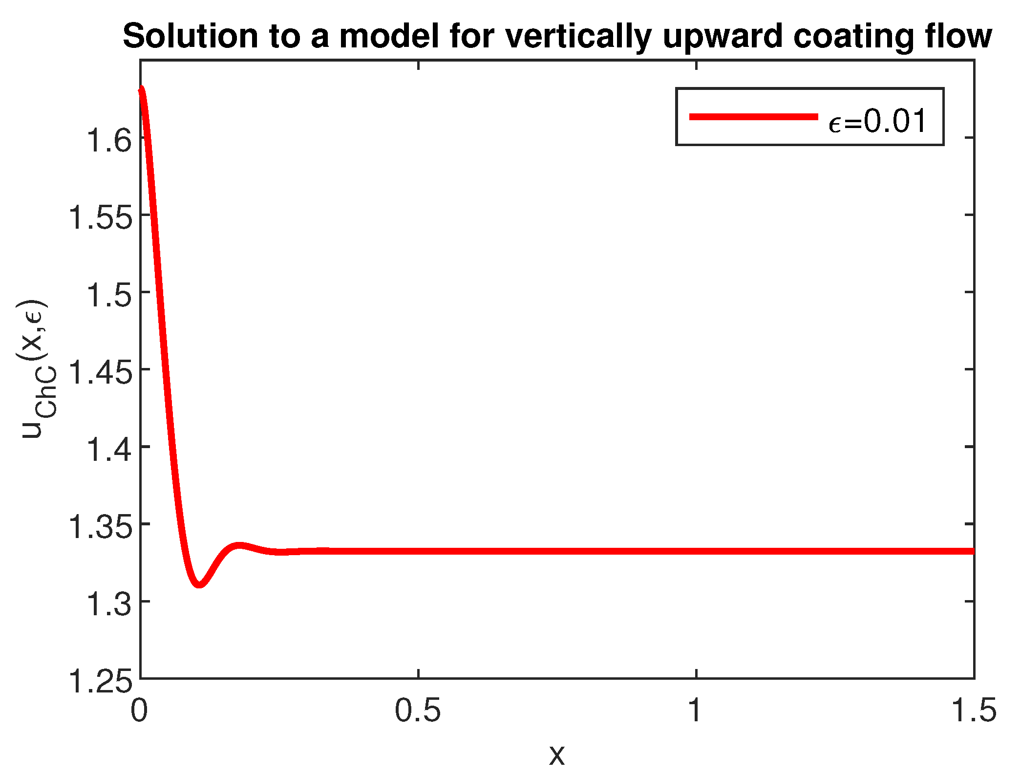
The solution to problem (16) is shown in Figure 9. An exterior boundary layer on the right of the origin is easily seen, which is in perfect concordance with the theory.

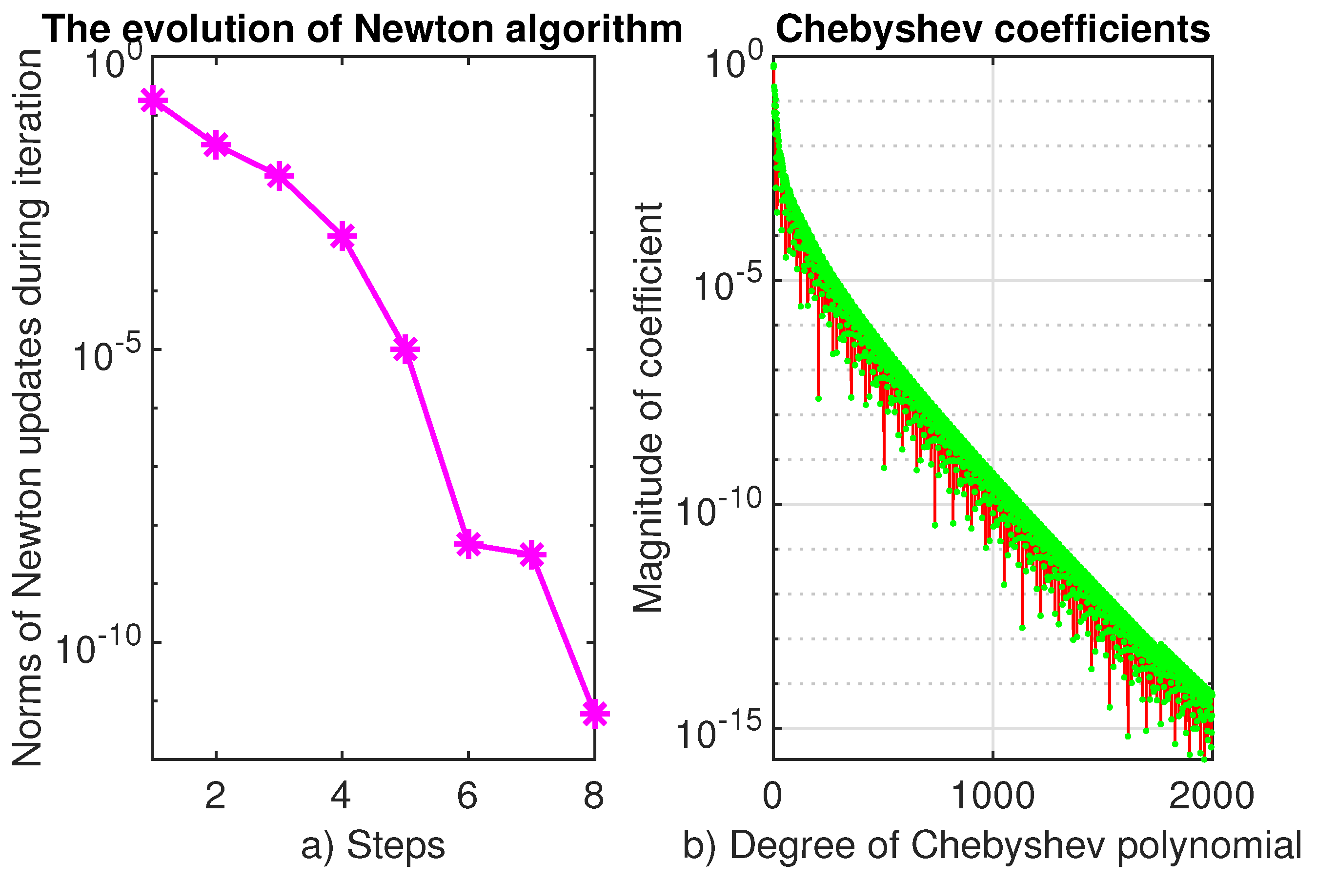
Newton’s method converges in 8 iterations, and its convergence order approximates two as seen from the left panel (a) of Figure 10. A more precise computed value reads $p:=1.81$. The right panel (b) of this figure indicates that Chebfun’s convergence rates for this problem decrease to subgeometric. The cause of this degradation is the appearance of the singularity ${\epsilon }^2$ in the left-hand side of the differential equation in (16).

The accuracy defined by (6) is of order ${10}^{-8}.$

3.5. An Upward Air Flow Which Can Support a Thin Layer of Liquid on a Plane Wall Against Gravity

Such stationary layers are, for example, sometimes seen on the windscreen of a car traveling at high speed in the rain.

Thus, we will consider now the following boundary value problem on the half line:

$$\begin{array}{c}{u}_{xxx}=u_x-u^{-1},x\in (0,\infty )\\ u\left(0\right)=u_x\left(0\right)=0\mathrm{and}u\to \sqrt{2x}\mathrm{as}x\to \infty .\end{array}$$

(17)

Its Chebfun solution is depicted in Figure 11, and it is perfectly similar to that displayed in [24].

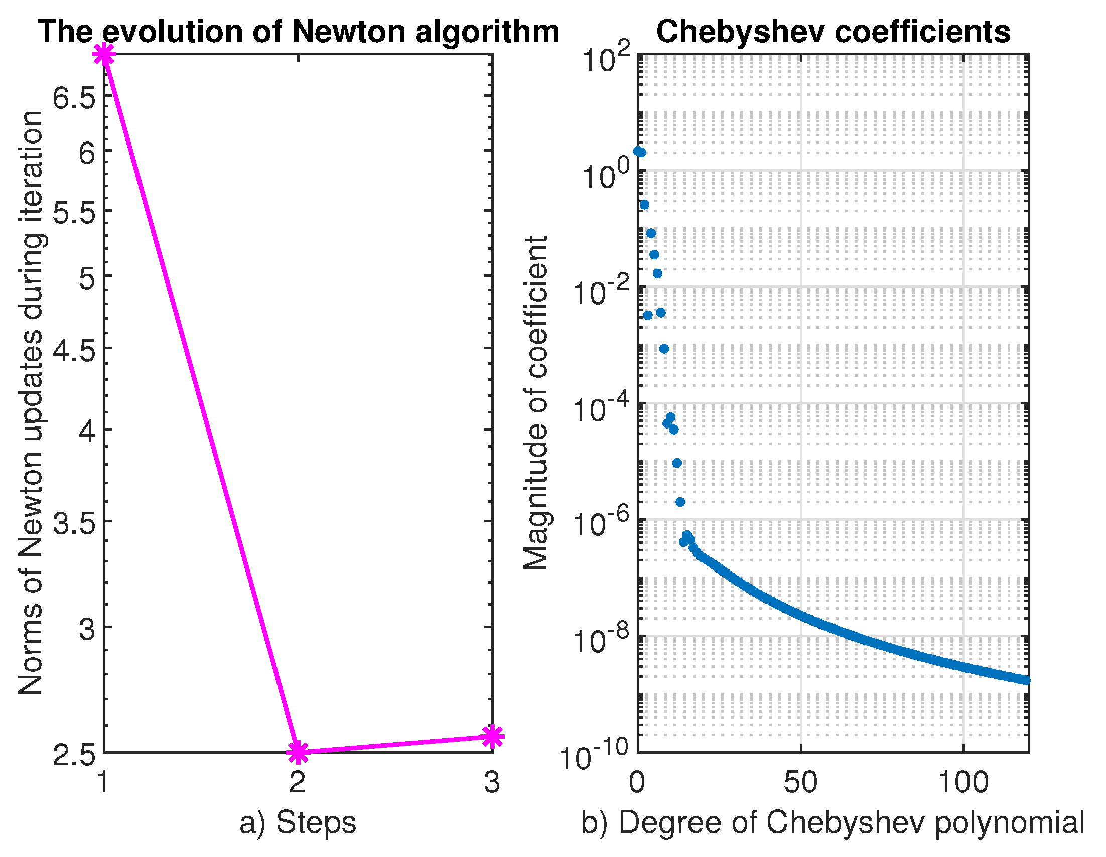
Solving this problem, we encountered the worst situation both in terms of accuracy and evolution of Newton’s algorithm.

As can be seen from the left panel (a) of Figure 12, immediately after switching on, Newton’s method ends in three iterations. The computed order equals $p=1.02$. The right panel (B) of this figure suggests that we cannot expect a better convergence than an algebraic one.

The accuracy remains at a very bad value, namely $8.745571373331746e-01$, which has not happened in any of the previous examples.

4. Conclusions

First, we must accept that Chebfun is not a panacea. However, it has been demonstrated to be a highly effective tool for addressing the singularities associated with the unboundedness of the domain or those intrinsically present in such challenging problems.

In addition to the reliable solutions obtained, we also obtained precise information on the errors committed. In this respect, we believe that Chebfun surpasses all existing methods.

In the literature, it is considered that subgeometric convergence rarely occurs when solving problems on finite domains but is normal when working on unbounded domains. However, in at least two cases, Chebfun showed that this convergence can even be geometric.

The overall results represent a confirmation of our opinion, formulated in [4,25], that spectral collocation-type methods can successfully replace shooting and finite-difference methods in solving boundary value problems on unbounded domains.

An important collateral result is regarding the order of convergence of the Newton method for solving nonlinear algebraic systems. Specifically, we coupled a graphical method with an asymptotic numerical method to establish the order of convergence of this method with greater accuracy.