Abstract
Lifetime reproductive output (LRO), also called lifetime reproductive success (LRS) is often described by its mean (total fertility rate or net reproductive rate), but it is in fact highly variable among individuals and often positively skewed. Several approaches exist to calculating the variance and skewness of LRO. These studies have noted that a major factor contributing to skewness is the fraction of the population that dies before reaching a reproductive age or stage. The existence of that fraction means that LRO has a zero-inflated distribution. This paper shows how to calculate that fraction and to fit a zero-inflated Poisson or zero-inflated negative binomial distribution to the LRO. We present a series of applications to populations before and after demographic transitions, to populations with particularly high probabilities of death before reproduction, and a couple of large mammal populations for good measure. The zero-inflated distribution also provides extinction probabilities from a Galton-Watson branching process. We compare the zero-inflated analysis with a recently developed analysis using convolution methods that provides exact distributions of LRO. The agreement is strikingly good.
1. Introduction
Lifetime reproductive output (LRO), also known as lifetime reproductive success (LRS) is the number of offspring produced over an individual’s lifetime. When measured in terms of female offspring of females, and when mortality of the mother is accounted for, the expectation of LRO is the net reproductive rate (or NRR). When both male and female offspring are counted and maternal mortality is eliminated, the expectation of LRO is the total fertility rate (TFR). Keilman et al. [1] has categorized measures of lifetime reproduction in terms of various possible combinations of sexes.
Lifetime reproductive “output” is an intentionally flexible term. LRO could be defined as children of either sex, or of both sexes, or based on maternal properties, or based on offspring properties such as the prevalence of medical conditions.
These most widely used measures of LRO ( and TFR) are means, and ignore the fact that LRO is a random variable, subject to chance variation due to the stochastic life of the mother and the stochasticity in reproduction at each age or stage. The variance in LRO is an important quantity in evolutionary demography because it may, or may not, provide a required ingredient for natural selection (a few examples: [2,3,4,5,6]).
Several research programs have developed demographic methods for computing the variance, skewness, and other statistics of LRO from demographic models (life tables or matrix population models). One uses Markov chains with rewards (MCWRs) to compute as many moments of LRO as desired from the transition probabilities of an age- or stage-classified life history and the moments of stage-specific reproduction [7,8,9]. A second approach makes ingenious use of a convolution operation to generate a complete nonparametric probability distribution of LRO [10,11,12].
Two conclusions have emerged from this research program. First, when calculated from demographic models (life tables, matrix models, individual-based simulations) the life histories of humans, animals, and plants produce a great deal of variance in LRO. They do so even though the calculations explicitly apply the same demographic rates to every individual of each age or stage. In cases where the calculated variance can be compared to an empirical measurement, this individual stochasticity can account for a sizable fraction of the observed distribution (e.g., [6,13]). There is every reason to include variance in LRO in analyses of fertility, and yet it is seldom done.
Second, the distribution of LRO is usually positively skewed, in both calculations and in empirical measurements. Figure 1 shows a typical example of the distribution of LRO in the Black-Legged Kittiwake (Rissa tridactyla), a beautiful pelagic gull distributed in the northern waters of the Atlantic and Pacific oceans. More than half of the individuals produce no offspring at all, while a few produce many. The same positive skewness is routinely found in calculations, regardless of the methods used to calculate LRO (e.g., [4,5,7,8,11,13,14,15]). All these authors agree in suggesting that the skewness is at least partly due to the death of a fraction—sometimes a large fraction—of a cohort before reaching maturity, and hence failing to reproduce at all. We will refer to this as failure to mature.
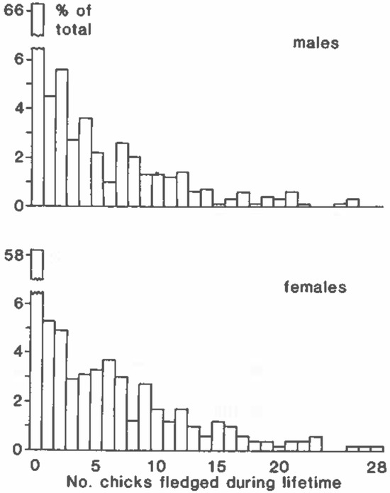
Figure 1.
Distribution of lifetime reproductive output in male and female Black-Legged Kittiwakes (Rissa tridactyla). From Thomas and Coulson [16] by permission of University of Chicago Press.
This paper will use demographic information on the probability of death before maturation to derive a parametric distribution for LRO, accounting for this source of zero-inflation. The goal is to see whether, and to what extent, this particular source of zero inflation can account for the skewness in the distribution of LRO. To do this, we will compare the results with the exact convolution method of Tuljapurkar et al. [11]. We do not claim that failure to mature is the only source of zero-inflation.
2. Notation
In this paper, matrices are written as upper case bold characters (e.g., ) and vectors as lower case bold characters (e.g., ). Vectors are column vectors by default; is the transpose of . The vector is a vector of ones, and the matrix is the identity matrix. When necessary, subscripts are used to denote the size of a vector or matrix, e.g., is an identity matrix of size . The symbol ∘ denotes the Hadamard, or element-by-element product (implemented by in Matlab and by * in R). Matlab notation will be used to refer to rows and columns of a matrix; e.g., and refer to the ith row and jth column of the matrix , respectively.
3. Zero-Inflated Distributions
The existence of a component of a cohort that dies before maturity implies that LRO has a zero-inflated distribution. A zero-inflated distribution is a mixture distribution with two parts [17,18,19,20]. One part is fixed at zero, the other is not. Zero-inflated distributions are also known as ‘cure models’ in survival analysis, to describe cases in time-to-event data where some individuals will never experience the event [21].
This paper presents a way to calculate zero-inflated distributions of lifetime reproductive output. Examples will be shown for recently developed countries, historical populations before the demographic transition, Hadza and Ache hunter-gatherer populations, and some other interesting cases.
Let be the probability distribution of the discrete variable X, which we consider as the LRO. If is zero-inflated, then
where
has a unit probability mass at , is the probability distribution of X conditional on it not falling into the zero-inflated category, and is the probability that X falls into the zero-inflated category. Note that may also include support at .
We present some facts about mixture distributions:
- The moments are also mixtures. Thus,where is the ith moment of the distribution , and similarly for , .
- All of the moments (except for that of order zero) of are zero.
- The moments of , the distribution conditional on survival to maturation, are
4. Calculating the Zero-Inflated Distribution
We describe demographic dynamics by an age- or stage-classified population projection matrix
where describes transitions of extant individuals and the production of new individuals by reproduction. In the age-classified cases in this paper, has age-specific survival probabilities on the subdiagonal and zeros elsewhere; has age-specific fertilities in the first row and zeros elsewhere. We will make use of the fact that the eventual population growth rate is the largest eigenvalue of .
- 1.
- We begin by generating the moments of LRO using the Markov chain with rewards (MCWR) method. You can generate as many as desired; here, we will consider the first moment (the mean), the second moment (which provides the variance), and the third moment (which provides the skewness) of the distribution . These moments of LRO are provided as vectors , , and , the calculation of which is given in Appendix A.1. The moments for ‘lifetime’ reproduction; i.e., starting from the first age class, are
- 2.
- Next, obtain the probability of failing to mature using the absorbing Markov chain created from . The transition matrix
 The matrix is written in column-to-row orientation and contains transition probabilities from living states to absorbing states. We create two absorbing states: the first corresponds to death before maturity, the second to maturity before death [22,23]. Define as the set of age classes for which fertility is greater than 0. An individual that reaches the set is absorbed in the ‘maturity before death’ absorbing state.The resulting mortality matrix isCreate a new transition matrix , which is equal to except that the that columns corresponding to are zero:Calculate the fundamental matrix corresponding to ,The matrix giving probabilities of absorption isRow 1 of gives the probabilities of death before maturity starting from each possible stage. Thus, starting from birth,The calculation is easily implemented in a few lines of Matlab code.
 - 3.
- Calculate the moments and statistics of the conditional distribution g from the moments of h and the probability of death before maturation, as in Equation (4),
- 4.
- Choose a distribution for g that can be parameterized by its moments. Here, we consider the Poisson distribution with parameter and the negative binomial with shape and scale parameterswhere denotes the variance.
5. The Convolution Method as a Standard of Comparison
The convolution method of Tuljapurkar et al. [11] partitions the population into groups defined by age at death. An individual who dies at age x contributes some number of offspring at each age up to x. The probability distribution of the sum of those contributions is the convolution of the probability distributions at each age up to age x. The final distribution of LRO, which we denote as , is the average of the convolutions over the distribution of ages at death. Stage-classified and time-varying models follow similar logic but are more complicated because of the greater variety of pathways possible through the life cycle.
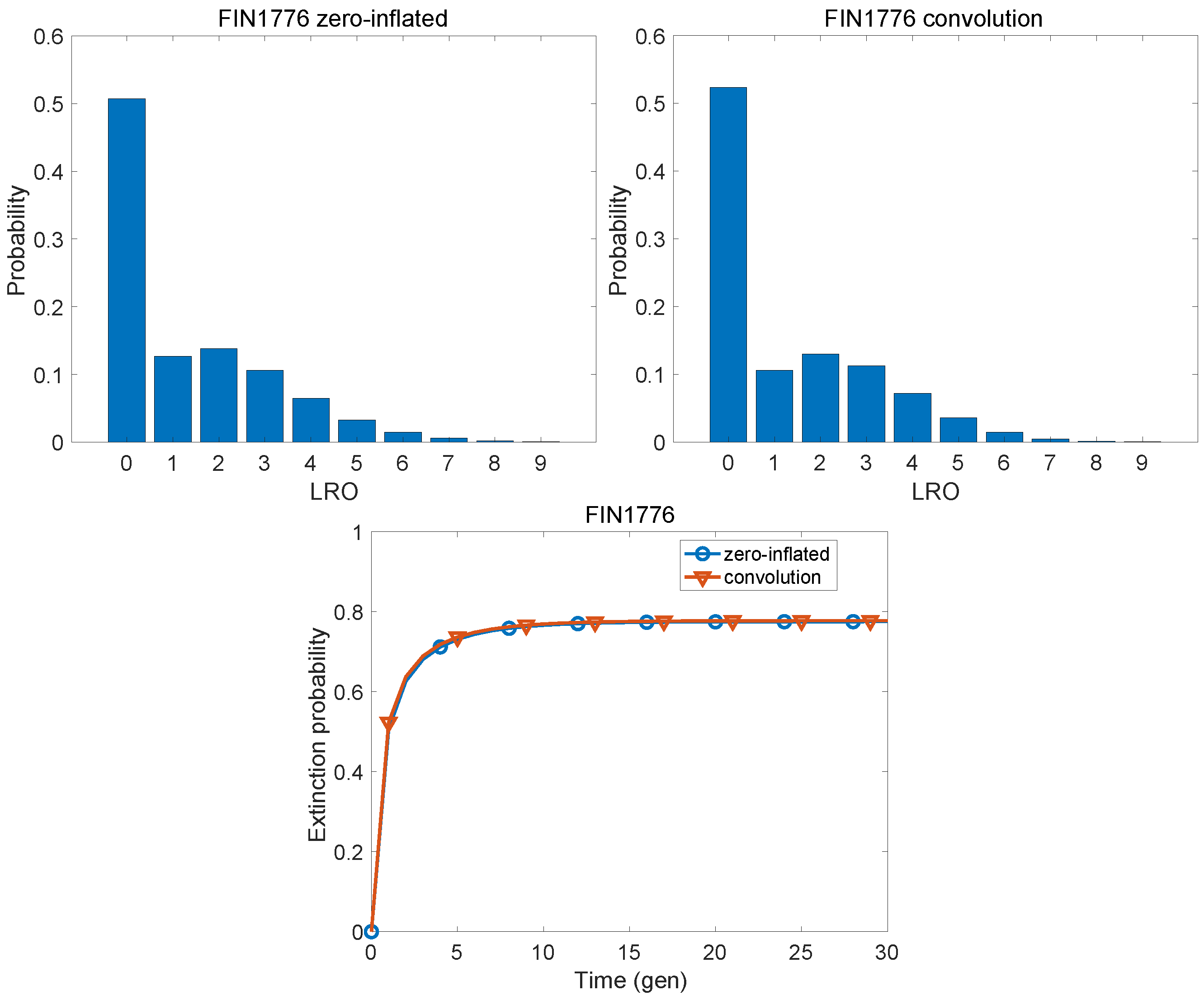
Because the convolution distribution makes no assumption about the parametric distribution of LRO, we use it as a standard of comparison for our zero-inflated distributions. In Figure 2, the zero-inflated and the convolution distributions appear quite similar. Their differences can be quantified with the Kullback–Leibler divergence (KLD; also called the relative entropy). Given two distributions, one (P) considered ‘true’ and one (Q) considered as a ‘model’ or approximation [24],
In our calculations, we treat the convolution result as the true distribution, and the zero-inflated distribution as a model
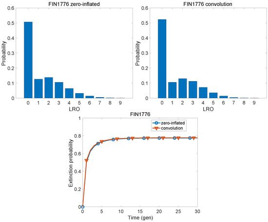
Figure 2.
Above: The probability distribution of LRO under mortality and fertility rates of Finland in 1776, as produced by a zero-inflated negative binomial distribution and by the exact convolution method. Below: The extinction probability of a lineage under these rates, in generations.
An Example
Turpeinen [25] presents mortality and fertility schedules for Finland starting in 1776. At this time, infant and child mortality was high, life expectancy at birth years, and the TFR was 5.4 children per woman. Using these data (also used in van Daalen and Caswell [6]) Figure 2 shows the results of the zero-inflated calculation of , compared to the exact distribution calculated from the convolution method. The probability of death before maturation was high (). The MCWR calculation gives a mean LRO of 1.30, a variance of 2.85, and a skewness of 1.16. The zero-inflated negative binomial distribution gives a conditional mean (conditional on survival to maturity) of 2.35, a conditional variance of 2.68, and a skewness of 0.52. Among individuals who survive to maturity, overdispersion is reduced by almost half (variance to mean ratio declines from 2.19 to 1.14) and skewness is reduced from 1.16 to 0.52. The interested reader may want to compare this distribution with the empirical distribution for the kittiwake in Figure 1.
The zero-inflated distribution does a good job of approximating the convolution result, with
which is an extremely close agreement between the two distributions.
6. Extinction
Extinction is one possible fate of a lineage started by a single individual, subject to specified mortality and fertility schedules. The classic Galton–Watson branching process permits the calculation of the probability of extinction. The calculation requires the probability distribution of the random number X of offspring produced to form the next generation (e.g., [26]). Tuljapurkar et al. [11] pointed out that because the convolution model provides the full distribution of LRO, rather than just the moments, it allows extinction probabilities to be calculated as a branching process, and Tuljapurkar and Zuo [10] have explored the implications for evolutionary demography.
The probability of extinction can be calculated as the smallest fixed point of the iterated probability generating function of LRO. The probability generating function
For the zero-inflated mixture distribution, the pgf is the weighted mean of the pgf for and for . Denote these by and ; then,
Extinction probability is usually presented as the solution to , which in the zero-inflated case is
An alternative is to calculate the probability of extinction as a recurrence over generations n. We have
with because the lineage is started by a living individual.
In the example of Finland, Figure 2 shows the dynamics of extinction probability for both the zero-inflated and convolution distributions. Despite the mean LRO (i.e., net reproductive rate) of 1.3, the asymptotic probability of extinction is ; the probability reaches nearly this value within 10 generations. The probabilities calculated from the zero-inflated and the convolution distributions are nearly identical.
7. Case Studies: A Gallery of Zero-Inflated Distributions
This section presents a series of estimates of the zero-inflated distribution of LRO and the corresponding distribution from the convolution method. The extinction probabilities are also compared for both methods. When the variance of is greater than the mean, is a zero-inflated negative binomial distribution (ZINB); when the variance is less than or equal to the mean, the distribution is a zero-inflated Poisson (ZIP), as indicated in the caption of each figure. Each figure also shows the time courses of the probabilities of extinction of a lineage founded by a single individual, calculated from each of the two distributions. Summary statistics are presented in Table 1 and Table 2.

Table 1.
The Kullback–Liebler divergence (KLD) between the zero-inflated approximation and the convolution result for the probability distribution of LRO and the probability of death before maturity.

Table 2.
The mean, variance, and skewness of lifetime reproduction from birth, calculated from the full zero-inflated distribution and from the distribution conditional on survival to reproduce.
7.1. Demographic Transitions
Many populations have passed through demographic transitions, from earlier conditions with relatively low survival and high fertility to more recent conditions with high survival and low fertility. The next figures show examples, based on rates from the Human Mortality Database [27] and Human Fertility Database [28].
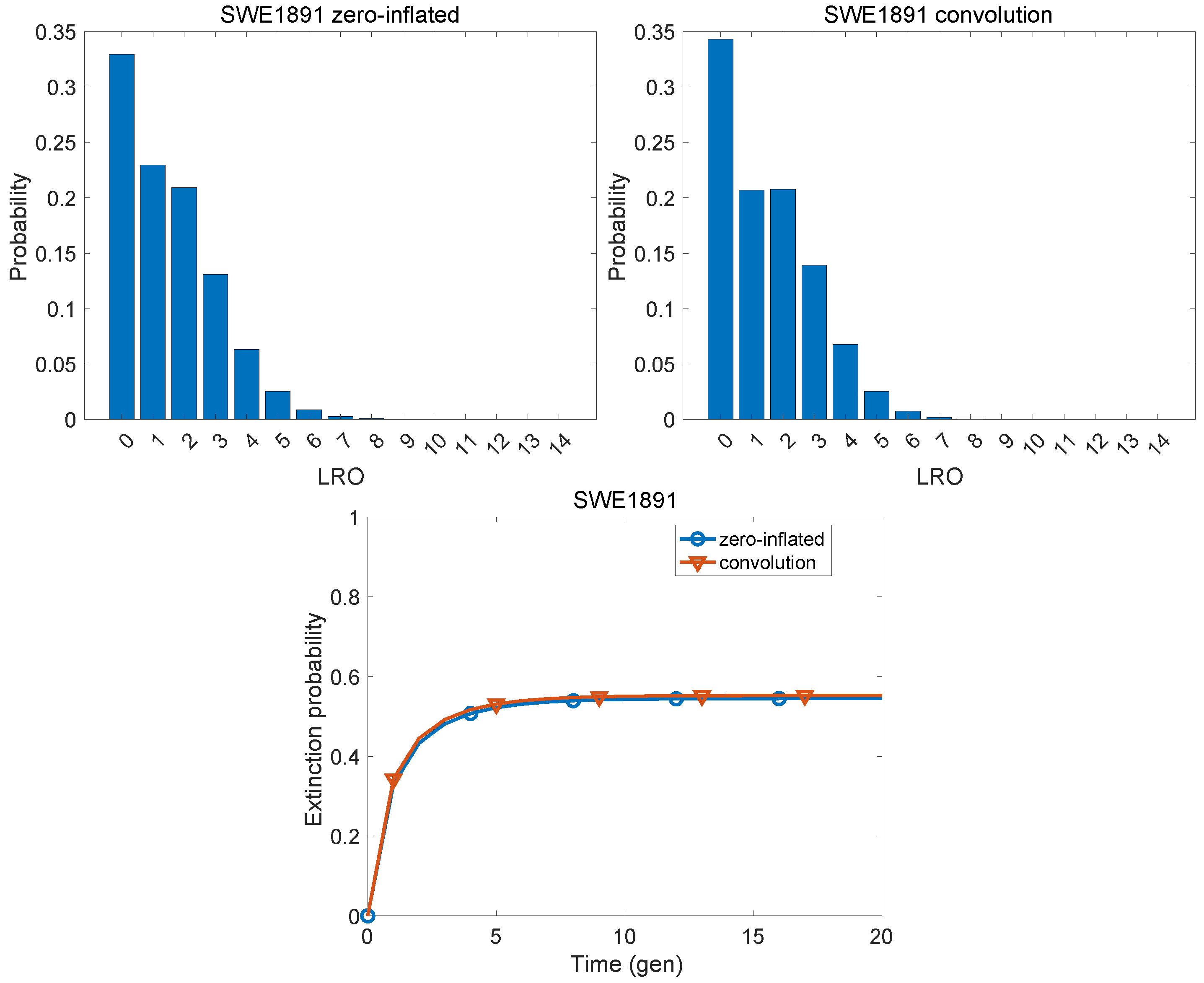
Figure 3 shows the probability distribution of LRO for Swedish females under 1891 rates, with TFR = 4.13, years, and the probability of death before maturity . The distribution calculated by the zero-inflated distribution is very similar to that produced by the convolution method (KLD = 0.0032) and the trajectories of extinction probability implied the two distributions are indistinguishable.

Figure 3.
The probability distributions of LRO calculated from the ZINB model and the exact convolution method, and the dynamics of extinction probability, under the mortality and fertility rates of Sweden in 1891.
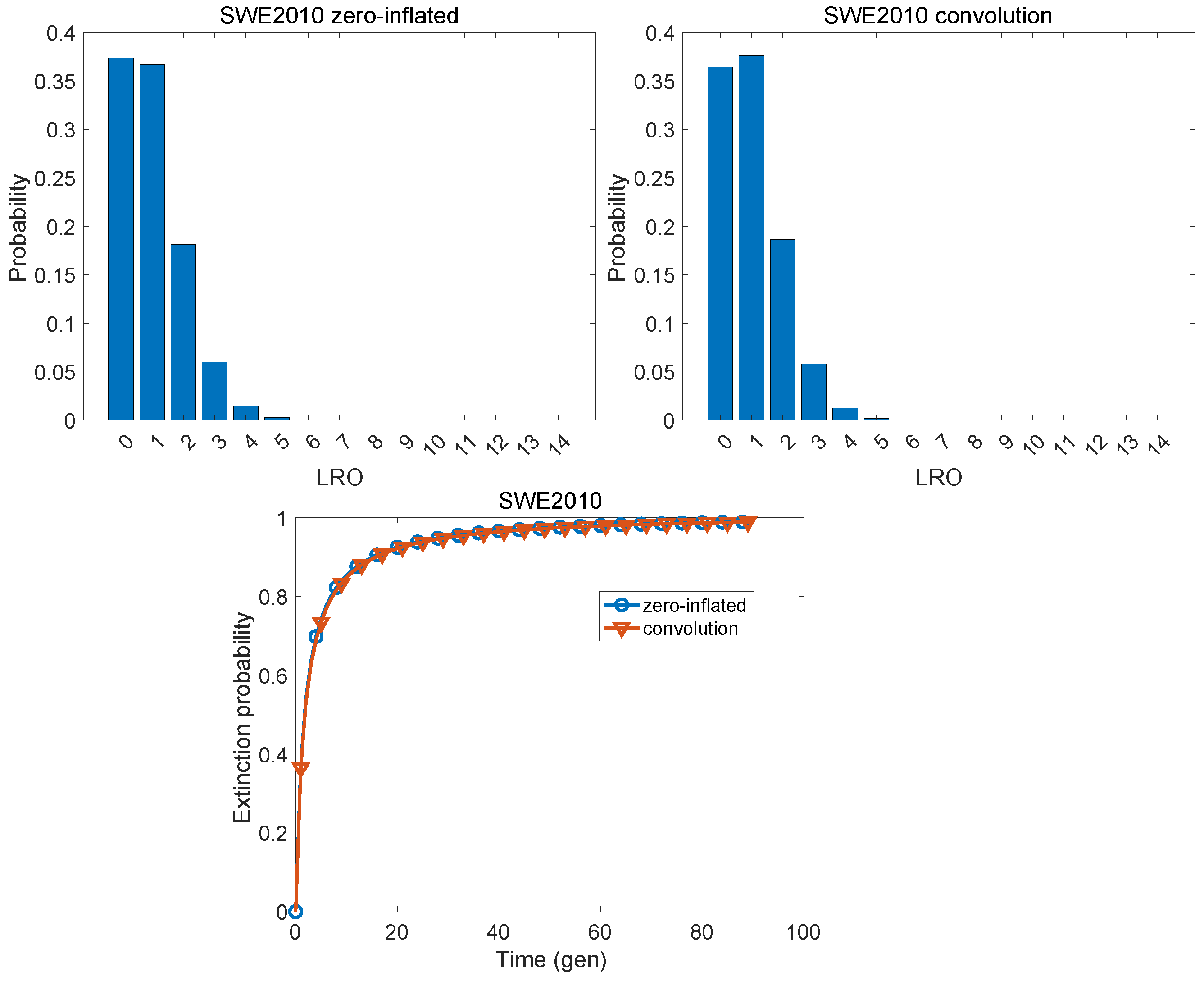
The rates for 2010 (Figure 4) reflect a population with very high survival () and low fertility (TFR = 1.99), slightly below replacement level (population growth rate ). Death before maturity is almost non-existent (). Again, the distributions of LRO are very similar (KLD = ). Because fertility is below replacement, the eventual extinction probability is 1; the trajectories from the two distributions are almost identical.
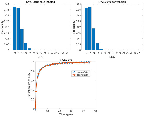
Figure 4.
The probability distributions of LRO calculated from the ZIP model and the exact convolution method, and the dynamics of extinction probability, under the mortality and fertility rates of Sweden in 2010.
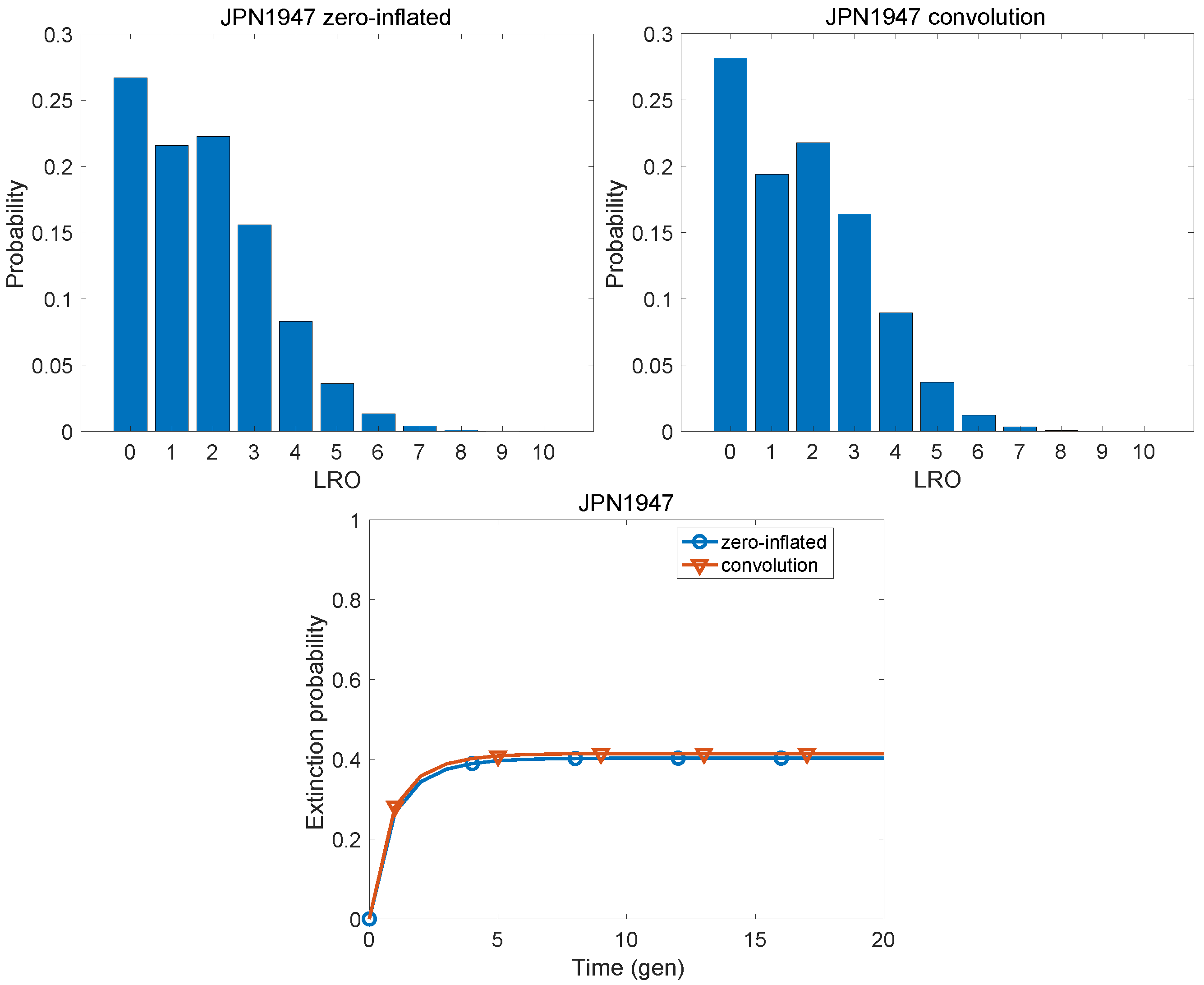
Japan underwent a similar transition between 1947 and 2019. Figure 5 shows the results under 1947 rates. Survival was low ( years) and fertility relatively high (TFR = 4.6). Death before maturity was fairly common (). The zero-inflated and the convolution distributions of LRO are quite similar (KLD = 0.0036), and the trajectories of extinction probability are almost identical.

Figure 5.
The probability distributions of LRO calculated from the ZINB model and the exact convolution method, and the dynamics of extinction probability, under the mortality and fertility rates of Japan in 1947.
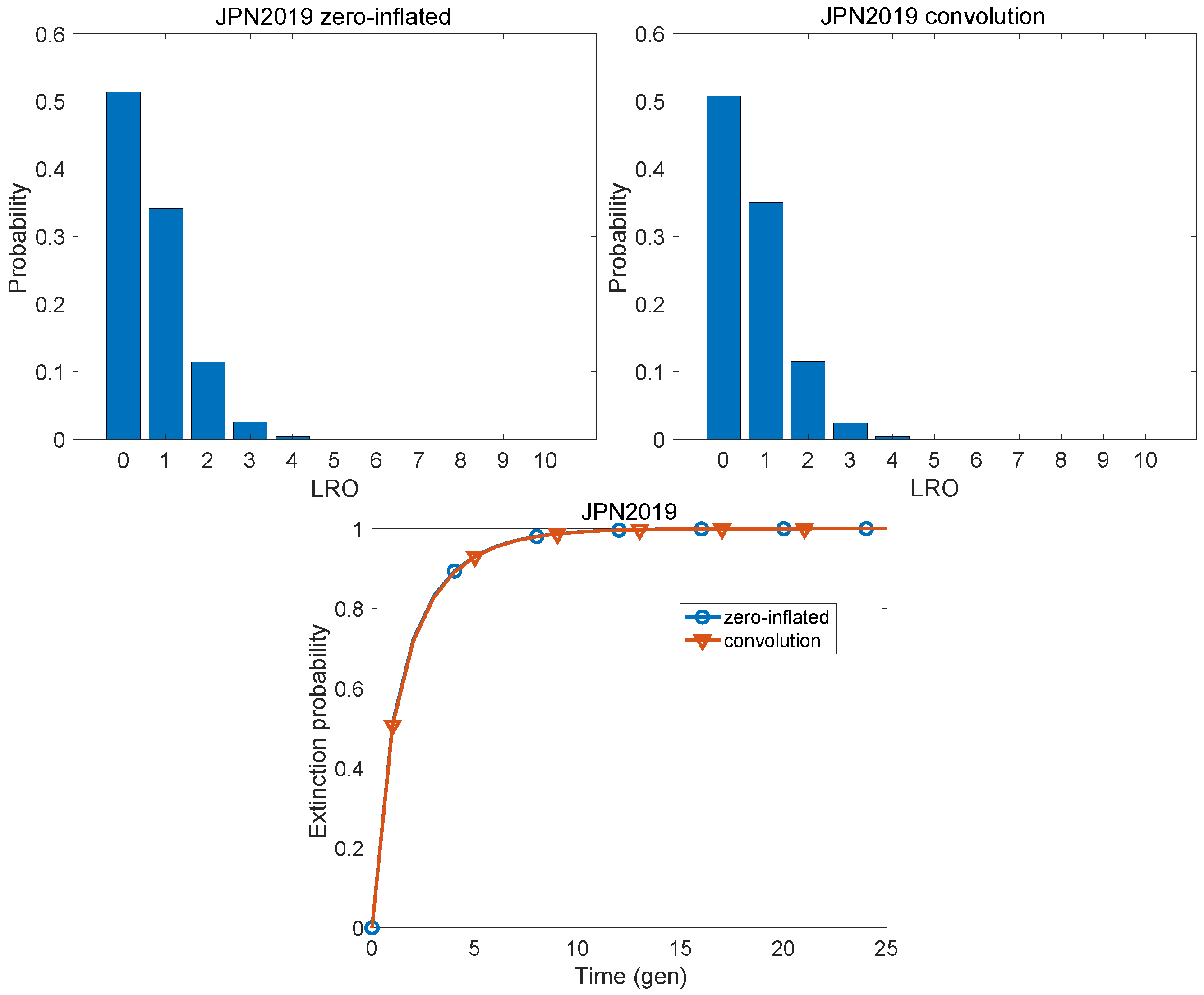
Under 2019 rates Japan had one of the highest life expectancies ( years) and lowest fertilities (TFR = 1.3) of any country. Death before maturation was almost nonexistent (). Figure 6 shows the distributions of LRO, which are very similar (KLD = ). As in the case of Sweden in 2010, eventual extinction is certain, and the trajectories of extinction probability are nearly identical.
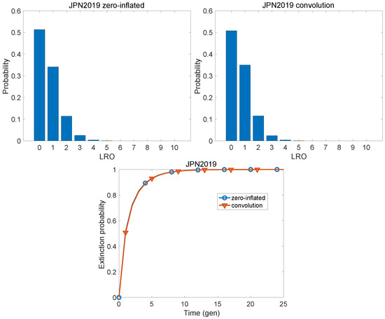
Figure 6.
The probability distributions of LRO calculated from the ZINB model and the exact convolution method, and the dynamics of extinction probability, under the mortality and fertility rates of Japan in 2019.
7.2. Extremes of Fertility and Mortality
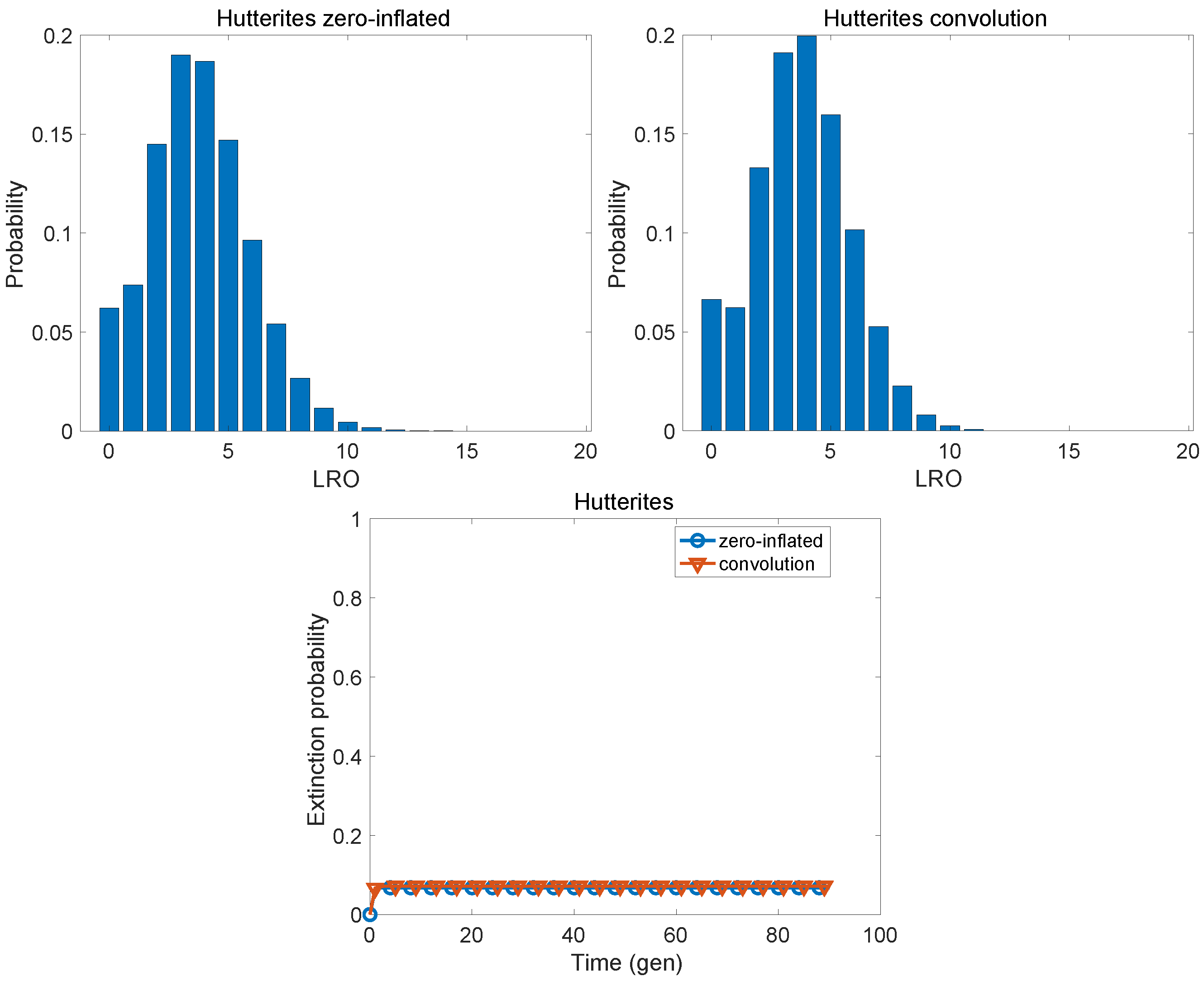
The Hutterites (members of an anabaptist religious community) have been recorded to have extraordinarily high fertility [29] with TFR = 8.1 and relatively high survival (, ). The combination yields a high population growth rate (). Figure 7 shows the distribution of LRO and the very low extinction probability for this population. The two distributions are very similar (KLD = 0.0071).
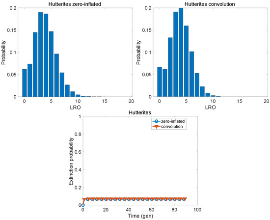
Figure 7.
The probability distributions of LRO calculated from the ZIP model and the exact convolution method, and the dynamics of extinction probability, under the mortality and fertility rates of the Hutterites.
Zero-inflation in this model is based on the risk of death before maturation. Figure 8, Figure 9 and Figure 10 show results for three populations with increasing probabilities of such early death.
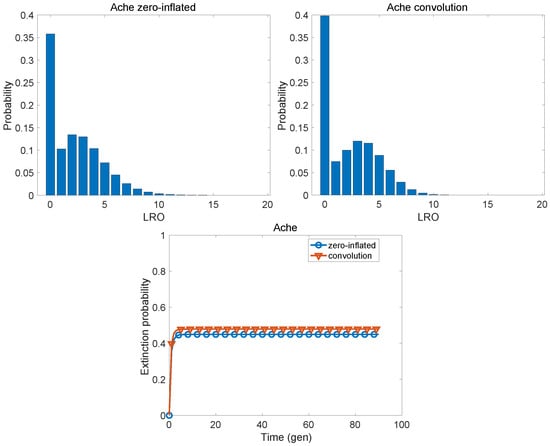
Figure 8.
The probability distributions of LRO calculated from the ZINB model and the exact convolution method, and the dynamics of extinction probability, under the mortality and fertility rates of the Ache hunter-gatherers.
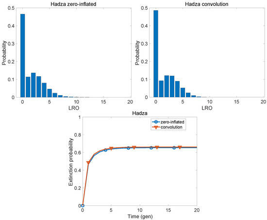
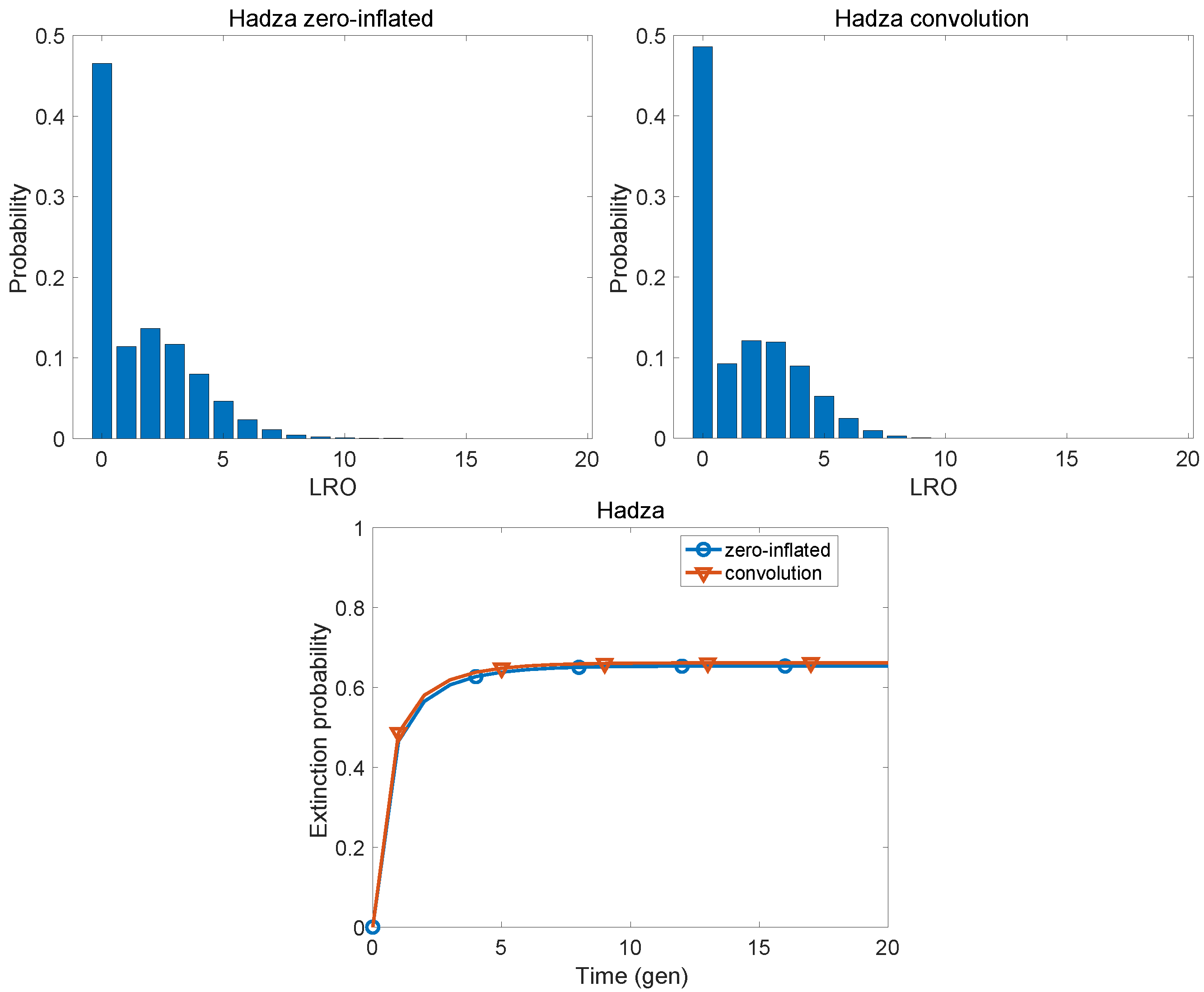
Figure 9.
The probability distributions of LRO calculated from the ZINB model and the exact convolution method, and the dynamics of extinction probability, under the mortality and fertility rates of Hadza hunter-gatherers.

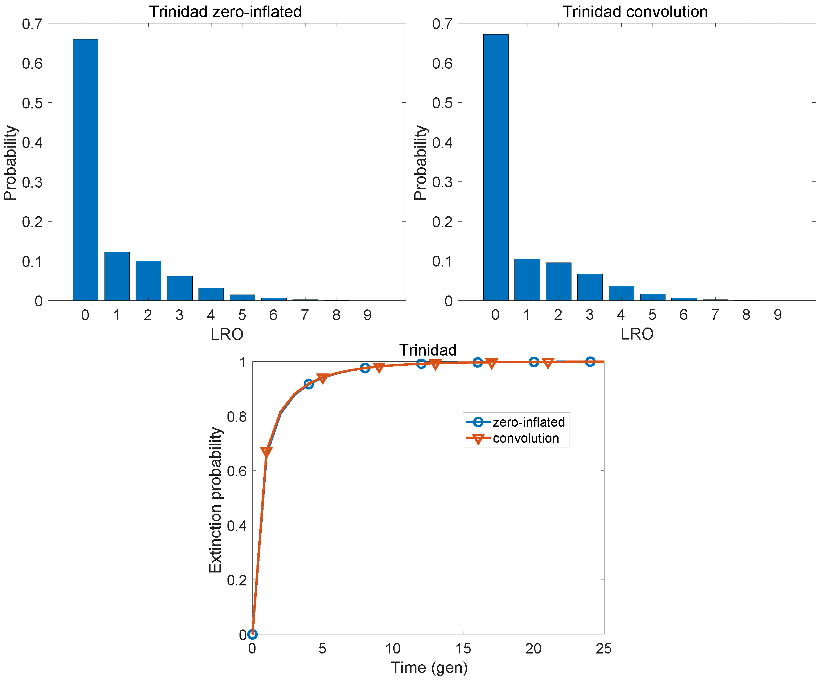
Figure 10.
The probability distributions of LRO calculated from the ZINB model and the exact convolution method, and the dynamics of extinction probability, under the mortality and fertility rates of plantation slaves in Trinidad, 1813–1816.
The Ache hunter-gatherers of subtropical Paraguay [30,31] have low survival ( years), with . Fertility as measured by TFR is high (TFR = 8.03), but as measured by net reproductive rate is only 2.2. The distributions of LRO are shown in Figure 8. The zero-inflated and the convolution distributions are close (KLD = 0.026), but not as similar as some other populations examined here. The extinction dynamics are similar, but the convolution calculation gives a slightly higher probability.
The Hadza hunter-gatherers of Tanzanian savanna [32] have a lower life expectancy and higher probability of death before maturity than the Ache; , . Figure 9 shows the distributions of LRO and extinction probability. The distributions are very similar (KLD = 0.008) and extinction probabilities are nearly indistinguishable.
Plantation slaves on the island of Trinidad in the early 19th century were subject to absolutely horrible conditions. John [33] calculated mortality and fertility schedules from slave registration records from 1813 to 1816, and concluded that “[t]he plight of the plantation slaves in Trinidad may be the most dismal known for any reliably reported population”. Based on data from Tables 6.3 and 7.6 of that book, I calculate a life expectancy of only years and probability of death before maturity of . The distributions, and , of LRO are shown in Figure 10; the two models produce very similar results (KLD = 0.0036). The ultimate extinction probability is, unsurprisingly, 1, and the two models give indistinguishable results for extinction.
7.3. Non-Human Populations
Interest in the statistics of LRO is not confined to human populations; here are two examples of the zero-inflation model applied to large mammals.
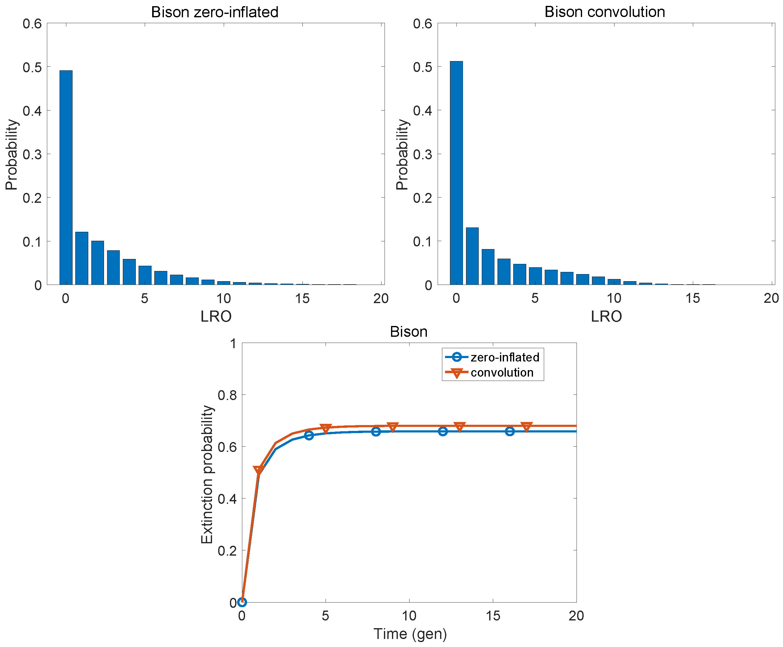
After near extirpation by the end of the 19th century, the American bison (Bos bison) is now found in scattered populations in central and northern North America. Brodie [34] reviews life history and demographic information bison from several long-term studies and provides quadratic logistic regression equations for age-specific survival and reproduction (Figures 1 and 3 of his paper). Figure 11 compares the distributions of LRO (KLD = 0.024).
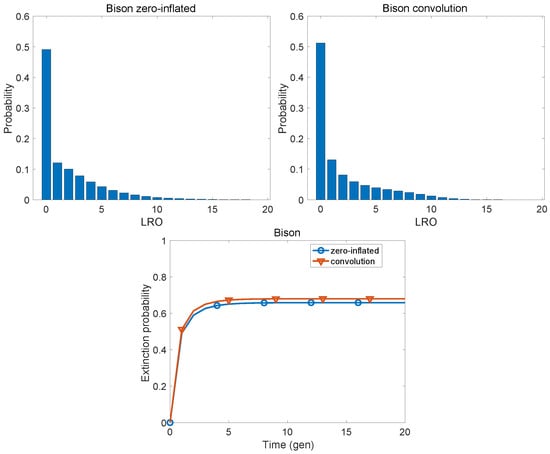
Figure 11.
The probability distributions of LRO calculated from the ZINB model and the exact convolution method, and the dynamics of extinction probability, under the mortality and fertility rates of the American bison (Bos bison).
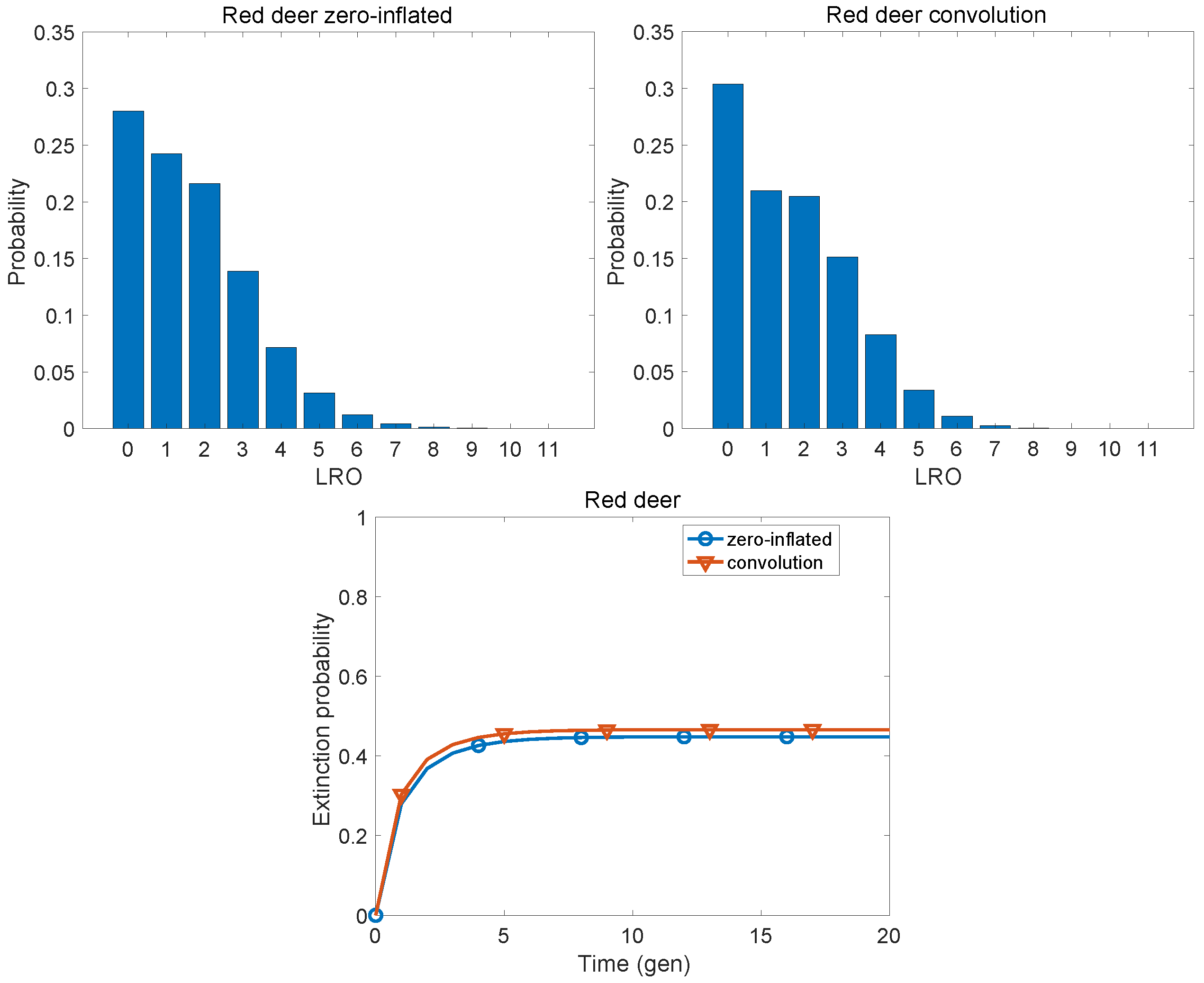
The red deer (Cervus elaphus) has been studied for many years on the island of Rum, Scotland. Benton et al. [35] reports survival and fertility results based on 21 years of longitudinal data. Figure 12 compares the distributions of LRO, which are quite similar (KLD = 0.0091), as are the extinction probabilities.

Figure 12.
The probability distributions of LRO calculated from the ZINB model and the exact convolution method, and the dynamics of extinction probability, under the mortality and fertility rates of red deer (Cervus elaphis).
8. Discussion
The approach presented here uses the mortality schedule, in the form of a Markov chain, to calculate the probability of zero-inflation due to death before maturity. Together with the moments of LRO provided by the MCWR calculation, this gives the moments of the distribution of the distribution of LRO, conditional on survival. These moments make it possible to fit a Poisson or a negative binomial distribution to .
8.1. Stochasticity, Not Heterogeneity
It is important to keep in mind that the variance, skewness, and indeed the whole probability distribution of LRO reflect differences among individuals due to chance (stochasticity), not to any differences in the properties of those individuals (heterogeneity). This is because when LRO is calculated from a Markov chain, a Markov chain with rewards, or a life table, the calculations explicitly suppose that every individual is subject to the same rates and probabilities. This leaves only stochasticity as the source of the variation [36]. This has been known to confuse studies focused on inequality [37]. In order to capture heterogeneity among individuals in the rates to which they are subject, it is necessary to divide the population into groups (e.g., income groups) and calculate the statics of LRO in each group. Given that, there is a huge literature on how to partition the variance in any demographic outcome (often referred to as “inequality”) into contributions from heterogeneity and stochasticity.
The situation is different when the distribution of LRO is measured empirically by following individuals through their life, as is the case in the kittiwakes in Figure 1. Some of the variability in that figure is certainly due to the stochastic outcomes of survival and reproduction, but some of it is no doubt due to differences in the properties of the individual birds. As with the life table calculations, when sources of heterogeneity can be identified, it is possible to partition that variance into contributions from within-group stochasticity and between-group heterogeneity (e.g., [37,38,39,40]). This has important applications in analysis of variance in terms of Crow’s index of the opportunity for selection. Waples [41] have surveyed these analyses for a variety of life cycles and sampling designs, using zero-inflated distributions of LRO as null models.
8.2. Some Open Problems
- Doubly-inflated distributions. Failure to survive to maturity is not the only reason that an individual may have an inherently zero reproductive output. Other causes (e.g., infertility due to medical causes, failure to marry, joining certain religious orders) would make the distribution of LRO doubly inflated. In such a case, the conditional distribution would also be zero-inflated. Methods given in Böhning et al. [19] and Beckett et al. [18] may enable this second level of zero-inflation (and perhaps more) to be estimated.
- How to evaluate the fit of ? Some of the moments of will be used to estimate the parameters of the chosen distribution (Poisson or negative binomial here). The moments that are not used for estimation can provide some insight into the goodness of fit, but it is hard to know how to evaluate the comparisons, and the concept of statistical ‘significance’ does not apply. The Kullback–Liebler divergence between the zero-inflated and the convolution distribution quantifies the difference, but it is an open problem of how to evaluate this quantity (i.e., how big a difference is big?).
- One motivation for the zero-inflated distribution model is the possibility of calculating the sensitivity of and to changes in the demographic parameters. The sensitivities of all the moments of LRO, calculated from the MCWR, are known [8]. So are those of the Markov chain from which is calculated [42,43]. It should be possible to apply these results to calculate the sensitivity of , , and to life history changes.
- Choosing a parametric distribution for is a challenge. The Poisson and negative binomial distributions are easy choices, inspired by the patterns shown in the first convolution-based analyses [11]. The negative binomial distribution is flexible in shape and reduces to, as special cases, the geometric or the Poisson distribution. There are several stochastic birth-death processes that lead to negative binomial distributions of population size [44,45,46]. Arguing purely by analogy, these might be relevant to the accumulation of offspring by an individual after reaching the set of reproductive stages.
- The zero-inflated calculations are unlikely to work when is not a well-behaved function. For example, the age-specific fertility of the polychaete Streblospio benedicti in laboratory culture is strongly bimodal (for unknown reasons, see [47]). This carries over to a bimodal distribution of LRO. The convolution method captures this nicely, but neither the zero-inflated Poisson nor the zero-inflated negative binomial does so (unpublished results). It is unknown how often such multimodal age-specific fertility schedules occur; dealing with them is an open problem.
- An interesting research problem is the application of the zero-inflated model to empirical measurements of lifetime reproduction (e.g., the kittiwake case of Figure 1), even without the availability of the age-specific mortality and fertility schedules needed for the MCWR or convolution calculations. There exist maximum likelihood estimates for the zero-inflated Poisson and zero-inflated negative binomial distributions, which may be useful [48,49].
8.3. Do We Need This?
The alert reader will have been asking whether we actually need this analysis. Do we need yet another way of calculating statistics of lifetime reproductive output? Several methods already exist. The MCWR method of Caswell [7], van Daalen and Caswell [8] includes stochasticity in both the lifetime of the individual and in the reproduction accomplished at each age or stage; it provides all the moments of LRO, is applicable to age- and stage-classified life cycles, and comes with a complete sensitivity analysis. The studies of Snyder and Ellner [4,50] take a similar approach but dig deeper into the life cycle and can attribute stochasticity to particular life stages and transitions. The convolution method [10,11,12] bypasses the calculation of moments and provides the complete probability distribution of LRO, in both age- and stage-classified life cycles.
So in one sense, no, we do not need zero-inflated distributions as yet another model for LRO. But there are at least three justifications for it. First, it is always good to have multiple ways to calculate a demographic outcome. Very often, different models or different calculations will provide different kinds of insights. Second, because the zero-inflated distribution is based on the MCWR calculation of moments, it is potentially amenable to sensitivity analysis, as described by van Daalen and Caswell [8]. It may lead to other analyses as well. Finally, zero-inflation due to death before reproductive maturity is a real demographic phenomenon, in some human and many animal and plant populations. Incorporating it explicitly invites a focus on its causes and how they relate to sociological and environmental conditions, especially in high mortality situations. It invites consideration of other causes as well.
Funding
Initial support provided by the European Research Council under the European Union’s Seventh Framework Programme (FP7/2007-2013), ERC Advanced Grant 322989 (INDSTOCH).
Institutional Review Board Statement
This paper does not require any ethics committee or review board approval because it uses only publicly available statistical data with no connection to any individuals and does not include any individual human data, samples, surveys, questions, or any other information subject to those approvals.
Informed Consent Statement
Informed Consent Statement was waived for this research because it uses only publicly available statistical data with no connection to any individuals and does not include any individual human data, samples, surveys, questions, or any other information subject to those approvals.
Data Availability Statement
No new data were collected in this study. All calculations were performed on published data available in cited locations.
Acknowledgments
The early stages of this research were supported by the European Research Council under the European Union’s Seventh Framework Programme (FP7/2007-2013), ERC Advanced Grant 322989 (INDSTOCH). The Distinguished Lorentz Fellowship from the Netherlands Institute of Advanced Study in the Humanities and Social Sciences provided funding for a workshop at the Lorentz Center of the University of Leiden on stochasticity. Discussion with S. van Daalen, L. De Vries, and N. Hartemink were important in developing ideas about lifetime reproductive output. I thank several anonymous reviewers for helpful comments.
Conflicts of Interest
The author declares no conflicts of interest.
Abbreviations
The following abbreviations are used in this manuscript:
| LRO | lifetime reproductive output |
| LRS | lifetime reproductive success |
| TFR | total fertility rate |
| life expectancy at birth | |
| KLD | Kullback–Leibler divergence |
| ZIP | zero-inflated Poisson distribution |
| ZINB | zero-inflated negative binomial distribution |
Appendix A
Appendix A.1. MCWR Calculation of the Moments of LRO
Note that some material in this Appendix is taken from Caswell and Zarulli [51] under terms of a CC-BY 4.0 International License.
The most direct and powerful way to calculate the moments of LRO is using Markov chains with rewards (MCWRs). These models were introduced by Howard [52] in stochastic dynamic programming. They have since been extended to calculation of LRO in demographic and life history models [6,7,8] and to studies of healthy longevity [51,53,54,55]. The population projection matrix
contains a matrix that is the transient matrix of an absorbing Markov chain. Let be the number of transient (living) states, the number of absorbing states, and the total number of states. The transition matrix of the Markov chain is then
 where is the matrix describing transitions from transient states to absorbing states (death or other ways of leaving the population).

As an individual moves among these states, it collects a “reward” when making the transition from state j to state i. The reward of interest here is reproductive output. These rewards accumulate over the lifetime of the individual; the accumulated reward at death is LRO. The reward is characterized by its moments, and appear in matrices that contain the first, second, and subsequent moments. For estimation of the reproductive rewards from various kinds of data, see Caswell [7], van Daalen and Caswell [8].
Let be a vector (dimension ) whose ith entry is the kth moment of the remaining lifetime reproductive output of an individual starting in state i. Because the dead do not reproduce, the entries of corresponding to absorbing states are zero. Thus, we obtain the complete statistics of LRO if we can find the moment vectors , where contains the first entries of , corresponding to the living stages. This vector is given by
where
in terms of this matrix, . We also define , the submatrix of corresponding to transitions among the transient states:
In terms of these quantities, the moments of LRO are given by the following expressions from Theorem 1 of [8]
and, in general,
where is the fundamental matrix of the Markov chain.
References
- Keilman, N.; Tymicki, K.; Skirbekk, V. Measures for human reproduction should be linked to both men and women. Int. J. Popul. Res. 2014, 1–10. [Google Scholar] [CrossRef]
- Clutton-Brock, T.H. Reproductive Success: Studies of Individual Variation in Contrasting Breeding Systems; University of Chicago Press: Chicago, IL, USA, 1988. [Google Scholar]
- Crow, J.F. Some possibilities for measuring selection intensities in man. Hum. Biol. 1958, 30, 1–13. [Google Scholar]
- Snyder, R.E.; Ellner, S.P. Pluck or luck: Does trait variation or chance drive variation in lifetime reproductive success? Am. Nat. 2018, 191, E90–E107. [Google Scholar] [CrossRef] [PubMed]
- Steiner, U.K.; Tuljapurkar, S. Neutral theory for life histories and individual variability in fitness components. Proc. Natl. Acad. Sci. USA 2012, 109, 4684–4689. [Google Scholar] [CrossRef] [PubMed]
- van Daalen, S.F.; Caswell, H. Demographic sources of variation in fitness. In Human Evolutionary Demography; Burger, O., Lee, R., Sear, R., Eds.; Open Book Publishers: Cambridge, UK, 2024; pp. 345–360. [Google Scholar]
- Caswell, H. Beyond R0: Demographic models for variability of lifetime reproductive output. PLoS ONE 2011, 6, e20809. [Google Scholar] [CrossRef] [PubMed]
- van Daalen, S.F.; Caswell, H. Lifetime reproductive output: Individual stochasticity, variance, and sensitivity analysis. Theor. Ecol. 2017, 10, 355–374. [Google Scholar] [CrossRef]
- van Daalen, S.F.; Caswell, H. Variance as a life history outcome: Sensitivity analysis of the contributions of stochasticity and heterogeneity. Ecol. Model. 2020, 147, 198856. [Google Scholar] [CrossRef]
- Tuljapurkar, S.; Zuo, W. Mutations and the distribution of lifetime reproductive success. J. Indian Inst. Sci. 2022, 102, 1269–1275. [Google Scholar] [CrossRef]
- Tuljapurkar, S.; Zuo, W.; Coulson, T.; Horvitz, C.; Gaillard, J.-M. Skewed distributions of lifetime reproductive success: Beyond mean and variance. Ecol. Lett. 2020, 23, 748–756. [Google Scholar] [CrossRef]
- Tuljapurkar, S.; Zuo, W.; Coulson, T.; Horvitz, C.; Gaillard, J.-M. Distributions of LRS in varying environments. Ecol. Lett. 2021, 24, 1328–1340. [Google Scholar] [CrossRef]
- Steiner, U.K.; Tuljapurkar, S.; Orzack, S.H. Dynamic heterogeneity and life history variability in the kittiwake. J. Anim. Ecol. 2010, 79, 436–444. [Google Scholar] [CrossRef]
- van Daalen, S.; Caswell, H. Lifetime reproduction and the second demographic transition: Stochasticity and individual variation. Demogr. Res. 2015, 33, 561–588. [Google Scholar] [CrossRef]
- van Daalen, S.F.; Hernández, C.M.; Caswell, H.; Neubert, M.G.; Gribble, K.E. The contribution of maternal age heterogeneity to variance in lifetime reproductive output. Am. Nat. 2022, 199, 603–616. [Google Scholar] [CrossRef] [PubMed]
- Thomas, C.S.; Coulson, J.C. Reproductive success of kittiwake gulls, Rissa tridactlya. In Reproductive Success; Clutton-Brock, T.H., Ed.; University of Chicago Press: Chicago, IL, USA, 1985; Chapter 16; pp. 251–262. [Google Scholar]
- Adarabioyo, M.; Ipinyomi, R. Comparing zero-inflated Poisson, zero-inflated negative binomial and zero-inflated geometric in count data with excess zero. Asian J. Probab. Stat. 2019, 4, 1–10. [Google Scholar] [CrossRef]
- Beckett, S.; Jee, J.; Ncube, T.; Pompilus, S.; Washington, Q.; Singh, A.; Pal, N. Zero-inflated Poisson (ZIP) distribution: Parameter estimation and applications to model data from natural calamities. Involv. J. Math. 2014, 7, 751–767. [Google Scholar] [CrossRef]
- Böhning, D.; Dietz, E.; Schlattmann, P. Zero-inflated count models and their applications in public health and social science. In Applications of Latent Trait and Latent Class Models in the Social Sciences; Rost, J.E., Langeheine, R., Eds.; Waxmann Verlag: Munster, Germany, 1997; Chapter 32; pp. 333–344. [Google Scholar]
- Haslett, J.; Parnell, A.; Sweeney, J. A general framework for modelling zero inflation. arXiv 2018, arXiv:1805.00555. [Google Scholar] [CrossRef]
- Amico, M.; Van Keilegom, I. Cure models in survival analysis. Annu. Rev. Stat. Its Appl. 2018, 5, 311–342. [Google Scholar] [CrossRef]
- Caswell, H. Matrix Population Models: Construction, Analysis, and Interpretation, 2nd ed.; Sinauer Associates: Sunderland, MA, USA, 2001. [Google Scholar]
- Caswell, H. Applications of Markov chains in demography. In MAM2006: Markov Anniversary Meeting; Boson Books: Raleigh, NC, USA, 2006; pp. 319–334. [Google Scholar]
- Cover, T.M.; Thomas, J.A. Elements of Information Theory, 2nd ed.; John Wiley and Sons: New York, NY, USA, 1999. [Google Scholar]
- Turpeinen, O. Fertility and mortality in Finland since 1750. Popul. Stud. 1979, 33, 101–114. [Google Scholar] [CrossRef]
- Harris, T.E. The Theory of Branching Processes; Springer: Berlin/Heidelberg, Germany, 1963. [Google Scholar]
- HMD. Human Mortality Database. Technical Report, University of California, Berkeley (USA), and Max Planck Institute for Demographic Research (Germany). 2022. Available online: www.mortality.org (accessed on 29 May 2025).
- Human Fertility Database. Max Planck Institute for Demographic Research (Germany) and the Vienna Institute of Demography (Austria). 2019. Available online: www.humanfertility.org (accessed on 29 May 2025).
- Eaton, J.W.; Mayer, A.J. The social biology of very high fertility among the Hutterites: The demography of a unique population. Hum. Biol. 1953, 25, 206–264. [Google Scholar]
- Gurven, M.; Kaplan, H. 2007. Longevity among hunter-gatherers: A cross-cultural examination. Popul. Dev. Rev. 2007, 33, 321–365. [Google Scholar] [CrossRef]
- Hill, K.; Hurtado, A.M. Aché Life History: The Ecology and Demography of a Foraging People; Aldine de Gruyter: New York, NY, USA, 1996. [Google Scholar]
- Blurton-Jones, N. Demography and Evolutionary Ecology of Hadza Hunter-Gatherers; Cambridge University Press: Cambridge, UK, 2016. [Google Scholar]
- John, A.M. The Plantation Slaves of Trinidad, 1783–1816: A Mathematical and Demographic Enquiry; Cambridge University Press: Cambridge, UK, 1988. [Google Scholar]
- Brodie, J.F. A Review of American Bison (Bos Bison) Demography and Population Dynamics; American Bison Society Working Paper 2; Wildlife Conservation Society: New York, NY, USA, 2008. [Google Scholar]
- Benton, T.G.; Grant, A.; Clutton-Brock, T.H. Does environmental stochasticity matter? Analysis of red deer life-histories on Rum. Evol. Ecol. 1995, 9, 559–574. [Google Scholar] [CrossRef]
- Caswell, H. Stage, age and individual stochasticity in demography. Oikos 2009, 118, 1763–1782. [Google Scholar] [CrossRef]
- Caswell, H. The contributions of stochasticity and social inequality to lifespan variability. Demogr. Res. 2023, 49, 309–354. [Google Scholar] [CrossRef]
- Hartemink, N.; Missov, T.I.; Caswell, H. Stochasticity, heterogeneity, and variance in longevity in human populations. Theor. Popul. Biol. 2017, 114, 107–117. [Google Scholar] [CrossRef]
- Tuljapurkar, S.; Edwards, R.D. Variance in death and its implications for modeling and forecasting mortality. Demogr. Res. 2011, 24, 497–526. [Google Scholar] [CrossRef]
- Vaupel, J.W. Inherited frailty and longevity. Demography 1988, 25, 277–287. [Google Scholar] [CrossRef]
- Waples, R.S.; Reed, T.E. Null models for the opportunity for selection. Am. Nat. 2023, 201, 779–793. [Google Scholar] [CrossRef]
- Caswell, H. Sensitivity analysis of discrete Markov chains via matrix calculus. Linear Algebra Its Appl. 2013, 438, 1727–1745. [Google Scholar] [CrossRef]
- Caswell, H. Sensitivity Analysis: Matrix Methods for Demography and Ecology. In Demographic Research Monographs; Springer Nature: Cham, Switzerland, 2019. [Google Scholar]
- Johnson, N.L.; Kotz, S.; Kemp, A.W. Univariate Discrete Distributions, 2nd ed.; Wiley: New York, NY, USA, 1993. [Google Scholar]
- Kendall, D.G. On some modes of population growth leading to R.A. Fisher’s logarithmic series distribution. Biometrika 1948, 35, 6–15. [Google Scholar] [CrossRef]
- Kendall, D.G. 1949. Stochastic processes and population growth. J. R. Stat. Soc. Ser. B (Methodol.) 1949, 11, 230–282. [Google Scholar] [CrossRef]
- Levin, L.A.; Caswell, H.; DePatra, K.D.; Creed, E.L. Demographic consequences of larval development mode: Planktotrophy vs. lecithotrophy in Streblospio benedicti. Ecology 1987, 68, 1877–1886. [Google Scholar] [CrossRef]
- Cohen, A.C. An extension of a truncated Poisson distribution. Biometrics 1960, 16, 446–450. [Google Scholar] [CrossRef]
- Cohen, A.C. A note on certain discrete mixed distributions. Biometrics 1966, 22, 566–572. [Google Scholar] [CrossRef] [PubMed]
- Snyder, R.E.; Ellner, S.P. We happy few: Using structured population models to identify the decisive events in the lives of exceptional individuals. Am. Nat. 2016, 188, E28–E45. [Google Scholar] [CrossRef] [PubMed]
- Caswell, H.; Zarulli, V. Matrix methods in health demography: A new approach to the stochastic analysis of healthy longevity and DALYs. Popul. Health Metrics 2018, 16, 8. [Google Scholar] [CrossRef]
- Howard, R.A. Dynamic Programming and Markov Processes; Wiley: New York, NY, USA, 1960. [Google Scholar]
- Caswell, H.; van Daalen, S.F. Healthy longevity from incidence-based models: More kinds of health than stars in the sky. Demogr. Res. 2021, 45, 397–452. [Google Scholar] [CrossRef]
- Dudel, C.; Myrskylä, M. Estimating the number and length of episodes in disability using a Markov chain approach. Popul. Health Metrics 2020, 18, 1–9. [Google Scholar] [CrossRef]
- Owoeye, S.M.; Oseni, B.M.; Gayawan, E. Estimating lifetime malnourished period and its statistics based on the concept of Markov chain with reward. Heliyon 2020, 6, e04073. [Google Scholar] [CrossRef]
Disclaimer/Publisher’s Note: The statements, opinions and data contained in all publications are solely those of the individual author(s) and contributor(s) and not of MDPI and/or the editor(s). MDPI and/or the editor(s) disclaim responsibility for any injury to people or property resulting from any ideas, methods, instructions or products referred to in the content. |
© 2025 by the author. Licensee MDPI, Basel, Switzerland. This article is an open access article distributed under the terms and conditions of the Creative Commons Attribution (CC BY) license (https://creativecommons.org/licenses/by/4.0/).


