Article

What Is the Evolution of Convergence in the EU? Decomposing EU Disparities up to NUTS 3 Level

by
Mindaugas Butkus
,
Diana Cibulskiene
,
Alma Maciulyte-Sniukiene
and
Kristina Matuzeviciute
*
Research Institute, Siauliai University, 77156 Siauliai, Lithuania
*
Author to whom correspondence should be addressed.
Sustainability 2018, 10(5), 1552; https://doi.org/10.3390/su10051552
Submission received: 11 April 2018 / Revised: 27 April 2018 / Accepted: 5 May 2018 / Published: 14 May 2018
(This article belongs to the Special Issue Economic Geography: Location, Innovation and Sustainable Development)

Abstract

:
Research on convergence deals with the question of whether regional disparities are decreasing over time. Aiming to decompose EU disparities covering regions of all levels, this paper fills the gap of the empirical research on convergence in the EU in the following ways: (i) the research updates the assessment of regional disparities in the EU emphasizing, but not limited to, the analysis at the NUTS 3 level; (ii) based on a constructed three-level Theil index, the research decomposes EU disparities into between-country, within-country at the NUTS 2 level, and within the NUTS 2 region at the NUTS 3 level components, covering the period of 1995–2014 and all EU regions, (iii) it examines the linkages between the development of innovation and technology, sustainability, and evolution of disparities. Our main findings suggest that convergence in the EU is still present at different regional levels, but its speed is slowing down. Total EU disparities were decreasing mainly because of reducing disparities between member states. At the same time, in the majority of EU member states, old and new, within-country disparities were growing at all regional levels, and now within-country disparities account for almost two-fifths of total EU disparities.

1. Introduction

By the beginning of the 21st century, the question concerning regional disparities had become one of the most relevant and controversial topics in economic and political debate. This was the result of the EU eastward enlargement encouraging the catch-up process of the new EU members. In fact, the results of studies on regional convergence for this period indicate that there was a tendency of absolute β-convergence in the EU. However, these studies also revealed the puzzle that convergence occurs at a national level, but not at a regional level—that is, variation of GDP per capita between countries decreases, while variation within countries mainly stagnates or even increases. One of the reasons to measure the level of convergence among EU regions is to evaluate the effectiveness of European Cohesion Policy. Many contributions examining the effect of Cohesion Policy on the convergence process inferred ambiguous findings. This encourages the further development of Regional Policy ensuring promotion of economic growth with social and institutional components not only at the national level but also at the regional level. Thus, convergence still remains a basic measure of the Cohesion Policy effectiveness.
Despite the considerable interest on the issue of regional disparities, the subnational level has attracted less attention as most of the empirical studies focus on the convergence issue in the EU at the NUTS 2 level. This phenomenon at the NUTS 3 level is mainly researched in southern and central eastern European countries [1,2,3,4,5,6,7,8,9,10,11,12,13], and old EU member states receive less attention [14]. Despite the increasing interest in convergence analysis at the NUTS 3 level during the last decade, studies encompassing the enlarged EU at the NUTS 3 level [15,16,17,18,19] are still rather scarce, keeping in mind that they confirm a significant increase in regional disparities at the NUTS 3 level.
The listed reasons determine the relevance of this research area, and our aim here is threefold: (1) to update the assessment of regional disparities in the EU, encompassing the most common instruments used in the analysis of convergence, emphasizing analysis at NUTS 3 level; (2) to decompose EU disparities into three components down to the NUTS 3 level, using a constructed three-level Theil index revealing more in-depth evolution of EU regional disparities, as well as to provide raw data on NUTS 3 disparities for 98 NUTS 1 regions, 276 NUTS 2 regions, and 28 EU member states over 1995–2014 for further research; and (3) to examine the nexus between development of innovation and technology, countries’ sustainability, and evolution of regional disparities.
The rest of the paper is organized as follows. Section 2 provides short theoretical introduction to convergence types along with some classical studies on EU empirics and summary of the recent studies of EU convergence at the NUTS 3 level. Section 3 introduces the alternative estimations of β-convergence and specifies inequality indices, emphasizing the Theil index decomposition. Section 4 provides the main empirical findings, focusing on the dynamics of disparities in the EU at the NUTS 3 level over 1995–2014. Section 5 concludes the paper.

2. Convergence Concepts and Brief Summary of Existing Empirical Evidence Concerning the EU

Different research methods are used to evaluate the process of convergence in the EU. Studies examining the process of the so-called β-convergence are based on neoclassical growth theory [20,21]. This concept was presented by Barro and Sala-i-Martin [22,23]. According to Barro and Sala-i-Martin, if all regions are converging to the same level of steady state, β-convergence is indicated. Barro and Sala-i-Martin [22] found that the process of convergence in European countries is similar to that in the United States and reaches about 2% a year. The early studies identified β-convergence among EU countries with low convergence speed [24,25,26,27,28,29,30,31]. Recent studies [32,33,34] indicate a higher convergence ratio, especially after enlargement of the EU in 2004. The estimated convergence indicators vary extensively, and they have changing signs. This neoclassical approach of convergence is under criticism for certain reasons. First, it is not usually tested using alternative models [35]. Second, factor mobility and other uncontrolled variables can influence detected β-convergence [36]. Third, small absolute convergence is indicated because regions have very different initial conditions. Recent studies [37,38,39,40,41,42] considered R&D expenditure as a key factor for regional convergence/divergence tendencies.
Another concept of Barro and Sala-i-Martin [43] is the σ-convergence approach, which means decreasing distribution of income across economies. The results of studies based on this approach are also contradictory. Some studies support the σ-convergence concept [16,44,45], while other studies [46,47,48,49] do not find evidence of σ-convergence in the EU.
The third concept of convergence—club convergence—is used to measure whether the groups of relatively homogenous regions converge to a similar steady-state value within the group but differ between groups. The concept of club convergence was introduced by Baumol [50]. The analysis of convergence clubs provides a more realistic and detailed picture about regional income growth than traditional convergence analysis. The concept of club convergence is related to Durlauf and Johnson [51] and Galor [52]. Borsi and Metiu [53] found four convergence clubs when analyzing data on the EU-27. The authors stated that convergence clubs are formed on the basis of geographic regions but are not related to membership in the Eurozone. Lyncker and Thoennessen [54] indicated club convergence in the EU-15, indicating a multispeed Europe along geographic regions, as income growth directions vary considerably among northern, central, and southern Europe. Table 1 summarizes empirical studies of convergence in the EU at the NUTS 3 level.
As it can be seen, there are only several studies covering most of EU regions at the NUTS 3 level [15,16,17,18,19,57,58,59] and there is no research that includes all NUTS 3 regions. Mostly southern and central eastern European regions are included in the research, excluding old members of the EU. Most empirical studies on convergence/divergence processes applied linear specification econometric or statistical models. It can be stated that studies confirm convergence in the EU. However, the analysis of convergence at the NUTS 3 level shows that disparities decreased at the country level but not at the regional level, and the speed of convergence varies over time. The results of empirical studies show different results, mainly affected by the particular method employed, the number of regions observed, and period covered.

3. Methodology and Data

Measuring convergence is, to some extent, a challenge, mainly because of two reasons: (i) there are several concepts of convergence, and even being related, they correspond to different aspects of the same process and thus it is necessary to take into consideration what is measured by one or another convergence index; (ii) there is no index to measure convergence that would allow to capture all aspects of this phenomenon, and that is why it is necessary to have in mind limitations of the existing indexes and to examine convergence in the EU, using different approaches and methodologies.
σ-Convergence, which is the main focus of this section, refers to the decrease of disparities between regions over time, while β-convergence focuses on finding possible catching-up processes.
To examine evidence of β-convergence in the EU at different regional levels, we estimated a few equations: one to test absolute β-convergence and another for testing conditional β-convergence. The difference between the two is that the latter includes additional variables to control the fact that regions initially have different growth conditions and probably will not converge to the same steady state. The equations of our interest are:
1 P p 1 l n ( y P , i y p , i ) = β 0 + β 1 l n ( y p , i ) + ε i
1 P p 1 l n ( y P , i y p , i ) = β 0 + β 1 l n ( y p , i ) + j = 1 k β j c j , i + ε i
where 1 P p 1 l n ( y P , i y p , i ) is the average annual growth rate of real per capita GDP (hereinafter per capita GDP or GDPpc) in region i over the period from p up to P. yp is the initial level of real per capita GDP and cj,i are the variables used to control different regional growth conditions. In our estimations of conditional convergence, we included dummy variables capital that is equal to 1 if capital city is situated in the region, costal that is equal to 1 if according to region typology it is a coastal region, urban that is equal to 1 if, according to rural–urban typology, it is assumed to be an urban region, and likewise for rural (intermediate is set as a benchmark region type), as well as country dummies. ε i is the error term assumed to be identically and independently distributed. β0 and β1 are the parameters to be estimated.
We did not intend to include all growth controls—such as human capital, investment, industry mix, institutions, and others—in our conditional convergence equation, partly because the main aim of our study is not to examine regional growth factors and partly because regional urban–rural typology and country dummies can also be used as a naive proxy for initial differences in growth condition.
Negative and statistically significant correlation between the initial level of per capita GDP and its growth rate over the next years (reflected as the estimated negative β 1 ) is the evidence of β-convergence. The time necessary for disparities to decrease by 50% can be calculated using formula:
l n 2 l n ( 1 + β 1 )  
Half-life period was calculated in cases when statistically significant convergence was detected.
The parameters β0 and β1 can be estimated, using different estimation methods. OLS estimation of Equations (1) and (2) could produce biased results for a few reasons. First, having no time dimension and analyzing regional data, we cannot assume that observations are independent. Even analyzing cross-sectional data at the regional level, we could find possible dependence which is spatial in nature. Closeness and various connections between surrounding regions could lead to reciprocally dependent regional economic variables that are not in line with the assumptions under which estimations of Equations (1) and (2) could be treated as valid. Thus, ignoring space in the analysis might produce omitted variable bias. Two common approaches are proposed to address this issue. One is to account in the equation for the fact that a region’s growth rate depends on growth rate (or income level) of neighboring regions using spatial lags (see, for example, [12,16]) in the spatial lag model (SLM). Another possible solution is to assert that spatial correlation of variables produces a possibility of systematic measurement errors and to consider a spatial error model (SEM) as an alternative model (see, for example, [6,11]).
Because economies of regions are fundamentally different, the second potential source of bias is spatial heterogeneity, which directly corresponds to the definition of convergence clubs. This type of convergence allows multiple, locally stable, steady-state equilibrium to which economies similar to each other are possibly converging. Convergence clubs would mean that relationships, expressed in absolute or conditional β-convergence equations, vary in space, and the true value of relationships is not stable over space and/or that variance–covariance of the error term varies across observations. We do not address the problem known as structural instability in our research. To overcome the group-wise heteroscedasticity problem, we used a heteroscedasticity corrected covariance matrix estimator.
It is, therefore, no surprise that the results of β-convergence analysis discussed in Table 1 are mixed and hardly comparable. They depend not only on the specification (absolute or conditional) adopted for β-convergence analysis or variables included in c (Equation (2)), or on period and the number of regions observed, they also strongly depend on adopted estimation strategy (incorporation of spatial effects, error corrections, etc.). Spatial dependency becomes stronger and more influential at smaller (NUTS 2 and NUTS 3) regional level and, thus, the usage of SLM or SEM is not very reasonable at the country or NUTS 1 level. Aiming to compare the results of convergence in the EU at different regional levels and to examine the evolution of convergence speed, we estimated Equations (1) and (2) using OLS, firstly, assuming that convergence between regions that are large in size (according to GDP or population) has the same effect on overall convergence as the convergence between regions that are small in size. Alternatively, we used weighted least squares (WLS) that enabled ascertaining weight of each region, as well as the influence of its growth on the overall convergence process.
The main source of the data is ESA 2010 (reg_eco10gdp), subsection for Gross domestic product (GDP) at current market prices by NUTS3 regions (nama_10r_3gdp). To correct the changes at price levels over time, we used Price index (implicit deflator), 2010 = 100, euro (PD10_EUR). For WLS estimations to calculate weights of the regions in the EU, we used Average annual population to calculate regional GDP data (thousand persons) by NUTS 3 regions (nama_10r_3popgdp). Data for per capita GDP and population in the aforementioned Eurostat data sources are not available prior to 2000. Data for 1995–1999 on Gross domestic product (GDP) at current market prices at NUTS level 3 and Average annual population was retrieved from nama_r_e3gdp and demo_r_d3avg datasets that were available on Eurostat previously and merged with currently available datasets. Information for NUTS 3 typologies and local information were collected from Regional typologies and local information corresponding to NUTS 3, according to NUTS 2010 codes.
Because the detection of β-convergence depends on the estimation of a specific model, and due to a number of other limitations of this approach, some researchers were encouraged to promote σ-convergence as more relevant to examine reality as it deals with a direct measurement of income distribution among regions. Besides the most commonly used summary indices of σ-convergence (i.e., standard deviation (SD) and coefficient of variation (CV) of per capita GDP at regional level), there exist more indices with different weighting schemes and implicit welfare functions applied, for example:
  • Gini coefficient (G), which is more sensitive when changes in inequality appear around the median;
  • Atkinson’s index (A), where weights to gaps between incomes in lower or upper tails of the distribution are assigned through the “aversion to inequality”;
  • Theil index (T) that gives equal weights across the distribution;
  • Mean logarithmic deviation (MLD), which is more sensitive to changes at the lower end of the distribution, while CV is more responsive to changes in the upper end of the distribution.
Because of different weighting schemes in use, these indices may not produce the same ranking of distributions, and evolution of disparities over time will probably not be the same for different indices. That is why it becomes crucial to analyze a variety of indices to conclude the extent to which disparities changes over time. In our research, we included four of them: CV, G, T, and MLD (for more details, see Appendix A). For each of these indices, disparities in the EU were measured at country, NUTS 1, NUTS 2, and NUTS 3 levels in terms of their per capita GDP, with the weights to the territories assigned according to their population share.
The Theil index—a particular case of the generalized entropy index with coefficient 1, which gives equal weights across the distribution—is of special interest in our research, because it has a “decomposability” property. Formally:
T(total EU disparities at NUTS 3 level) =
T(total disparities between countries) + T(total within countries disparities at NUTS 2 level) + T(total within NUTS 2 disparities at NUTS 3 level)
There are 1342 NUTS 3 level regions in the EU, each with different GDPpc denoted as yi3. The average GDPpc in the EU is y. There are Ni3 people living in each NUTS 3 region and the total EU population is N. All 1342 NUTS 3 level regions are distributed among 28 EU countries with per capita GDP and population denoted as yi0 and Ni0, respectively. Each country consists of R2 NUTS 2 level regions. yi2 denotes per capita GDP and Ni2 denotes population at the NUTS 2 level. Each NUTS 2 region consists of R3 NUTS 3 level regions with GDPpc denoted as yi3 and population denoted as Ni3. Thus, disparities in the EU at the NUTS 3 level can be measured and decomposed using Theil index:
T = i = 1 1342 ( N i 3 N y i 3 y l n ( y i 3 y ) ) = [ T 0 ] + [ i = 1 28 ( N i 0 N T 2 ) ] + [ i = 1 28 ( N i 0 N i = 1 R 2 ( N i 2 N i 0 T 3 ) ) ]
T0 measures disparities between 28 EU countries:
T 0 = i = 1 28 ( N i 0 N y i 0 y l n ( y i 0 y ) )  
T2 measures within-country disparities at the NUTS 2 level and is calculated for each country:
T 2 = i = 1 R 2 ( N i 2 N i 0 y i 2 y i 0 l n ( y i 2 y i 0 ) )
T3 measures within-NUTS 2 disparities at the NUTS 3 level and is calculated for each NUTS 2 region:
T 3 = i = 1 R 3 ( N i 3 N i 2 y i 3 y i 2 l n ( y i 3 y i 2 ) )
Alternatively, we decomposed the Theil index, substituting 28 EU member states with 98 NUTS 1 level regions (for explanation of decomposition, see Appendix B).

4. Empirical Findings

As it was mentioned in Section 2, convergence analysis mainly focuses on finding evidence of β- or σ-convergence. Quantitatively, we need to distinguish between β-convergence (referring to a process in which poor countries or regions are growing faster than rich ones and, therefore, are catching up with them) and σ-convergence (referring to a decrease of disparities among regions over time). β-convergence is necessary, but not sufficient, for σ-convergence. This section begins with discussing the evolution of disparities in the EU, using β- (Section 4.1) and σ-convergence (Section 4.2) concepts. The results of disparity decomposition are provided in Section 4.3. Section 4.4 examines the relationship between development of innovation and technology, sustainability, and evolution of disparities.

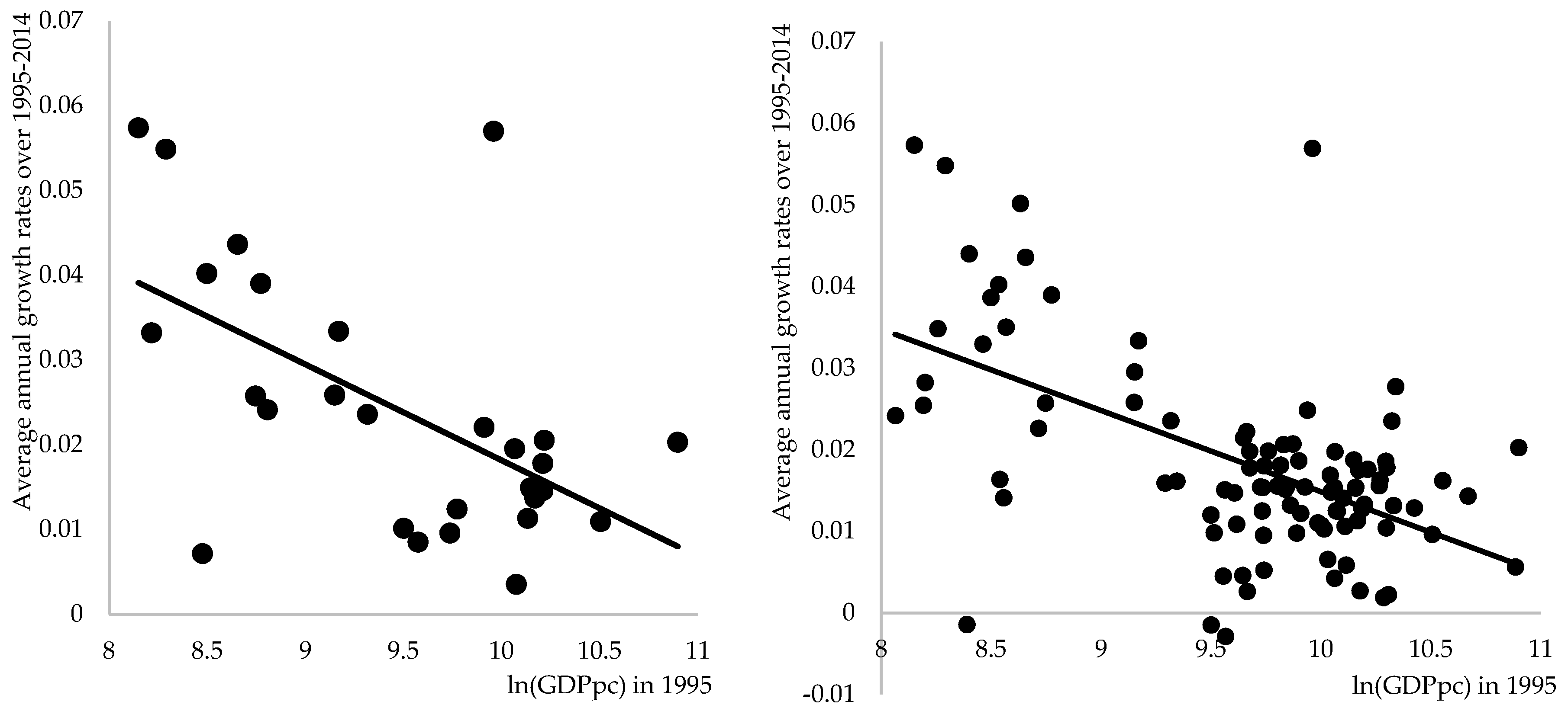
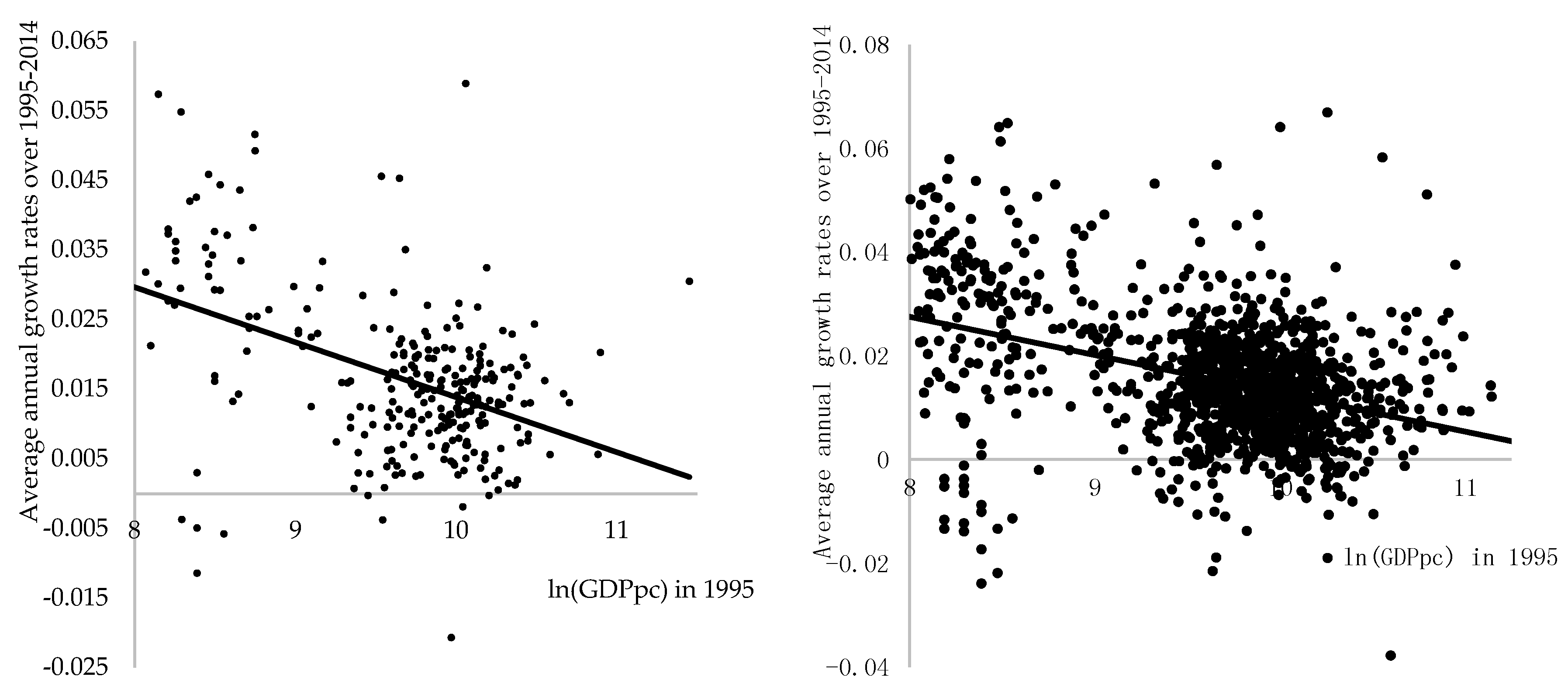
4.1. β-Convergence in the EU

The results of the estimations are discussed starting with the analysis of convergence between countries and subsequently going deeper into convergence between NUTS 3 regions in the EU. The convergence parameter is estimated for the whole 20-year period, as well as for some subperiods, to better capture an idea of how the convergence pattern is changing over time: (i) two 10-year subperiods, (ii) four 5-year subperiods, and (iii) two last 7-year EU funding programming periods of 2000–2006 and 2007–2013.
Over the past 20 years, β-convergence has been very strong between EU member states, as illustrated in Figure 1a. Countries that were poorer in 1995 grew faster than their richer neighbors over the next two decades. The average convergence speed during two decades was 1.13%. However, the speed of convergence was not constant over time, and evidence of convergence between EU member states is rather mixed (see Table A2 in Appendix C). For the period 1995–1999, the estimated convergence coefficient was insignificant. This was due to the fact that countries, which later became new EU member states, did not converge towards EU-15 countries in the late 2000s but converged strongly afterwards. The average speed of convergence during 2000–2004 was 2.21%, but decreased to 1.89% for the 2005–2009 period, and was only 1.25% for 2010–2014. This confirms the observation that convergence has lost its steam as differences among countries have become smaller and smaller, which is actually not very surprising.
The estimations of Equation (1) using WLS do not much change the general findings. Assigning weights to the countries according to their contribution to EU’s GDP or population share slightly increased the rate of convergence speed (see Table A2 in Appendix C) but did not change the fact that convergence is slowing down. The effect of faster growth, which is experienced by relatively poorer countries that joined the EU after 2004, compared to the EU-15 countries, maintained β-convergence but its impetus is running out.
NUTS 1 refers to major socioeconomic regions and, being larger than some of the smallest EU member states, they had patterns of absolute β-convergence similar to countries but at slightly slower speed. Over 20 years, the average speed of convergence was 1% (see Figure 1b) with no evidence of statistically significant convergence during the first 5-year subperiod, followed by significant 2.1% over 2000–2004, slightly decreasing to 2% for 2005–2009 and to 0.95% during the last subperiod (see Table A3 in Appendix C). Omitting from the estimations the regions with the largest (Luxembourg) and smallest (Macroregiunea doi, Romania) per capita GDP, we end up with a speed of convergence very similar to one observed at the country level. WLS estimates provide quite the same picture about patterns of absolute β-convergence between NUTS 1 regions.
Our estimations of the equation for conditional β-convergence between NUTS 1 regions include capital dummy and country fixed effects. Adding only capital dummy to the estimations did not change pattern or speed of convergence but revealed that capital regions grew on average faster by 0.95 p.p. per year compared to others (see Table A4 in Appendix C). Adding capital dummy markedly increased R-squared of the estimations, suggesting that capital city is an important growth factor through agglomeration effect. On the contrary, adding country fixed effect changed the whole picture. After controlling observable and unobservable differences in growth patterns at the country level, estimation revealed that convergence was insignificant during the whole 20-year period, and it was significant just for 2005–2009.
Going deeper (i.e., analyzing evolution of regional disparities at smaller scale) revealed that the convergence process is even slower at the regional scale and also losing its steam. NUTS 2 regions, which are the main focus of Cohesion Policy, were converging at an average speed of 0.8% for the whole 20-year period (see Figure 2a and Table A5 in Appendix C).
Breaking down analysis into 5-year subperiods, we observe significant absolute β-divergence (i.e., the opposite of convergence) for the period 1995–1999. This might be the case due to increasing differences between regions of old and new EU member states. Over the latter two 5-year subperiods, the estimated speed of significant absolute β-convergence was very similar at about 1.8%, which decreased more than 2-fold for the period 2010–2014, reaching just 0.8% (see Table A5 in Appendix C). After restricting our sample of NUTS 2 regions to 270 (we excluded the top and bottom three regions according to their average per capita GDP as the top one percentile and bottom one percentile of our sample, considered as extremes), the estimated speed of convergence between regions increased, but the dynamics of the process over the years remained the same (see Table A5 in Appendix C). Findings suggest that we can expect to observe faster convergence between more similar regions, which contradicts the core idea of absolute β-convergence—the bigger the initial differences among regions, the faster the speed of convergence. WLS estimates also revealed quite the same dynamics of absolute β-convergence, just at a slightly faster speed (see Table A5 in Appendix C).
OLS estimates of conditional β-convergence suggest that the effect of capital city on growth is bigger at a smaller scale. Over the 20-year period, NUTS 2 capital regions grew faster on average by 1.22 p.p. per year (compared to 1 p.p. in the case of NUTS 1 regions). Adding capital dummy to the model only slightly affected convergence speed over the whole and separate subperiods, but it increased R-squared, which is evidence of the importance of capital city effect on growth (see Table A6 in Appendix C). Augmenting the conditional β-convergence equation with the country dummies to control country fixed effects reduced speed of convergence to 0.47% over the 20-year period, but the estimated effect is still significantly contrary to what we observed at the NUTS 1 level. Breaking down analysis into subperiods revealed that significant convergence occurred for 2000–2004 and 2005–2009 at a speed of 1.2% and 0.7%, respectively.
We finish our analysis of β-convergence at the smallest, NUTS 3, regional level. We would like to stress here that, as we go in a deeper level (i.e., in smaller regional units), it is more likely that a notable part of regional GDP is assignable to commuters, thus the more inaccurate it becomes to use per capita GDP as a proxy for the regional per capita income. Addressing this inaccuracy is beyond the aim of our research, but it should be considered while examining regional disparities in terms of per capita GDP.
The estimated equation of absolute β-convergence, including all 1342 NUTS 3 regions, revealed that the speed of convergence in the EU over the 20-year period was 0.74% (see Table A7 in Appendix C), in other words, slower compared to what we observed at the NUTS 2, NUTS 1, or at the country level. It suggests that the deeper we go into the rabbit hole, the more stretched out the process of convergence appears. The analysis of evolution of regional disparities during separate subperiods revealed that the period of 1995–1999 is characterized as a period of divergence (as in case of NUTS 2 regions) with an estimated statistically significant speed of 0.59%. Latter periods were typically periods of significant convergence with a decreasing speed over time. Restricting our sample to 1313 regions (excluding the top 1 and bottom 1 percentiles of the extremes according to average per capita GDP), the speed of convergence slightly increased, but the pattern of disparities’ evolution remained the same.
Because NUTS 3 level regions are the smallest and, thus, mostly homogeneous, it was possible to control more characteristics at the regional level that might affect growth heterogeneity in the conditional β-convergence equation. Estimations provided in Table A8 (see Appendix C) show that capital and urban regions were growing faster on average by 1 p.p. and 0.32 p.p. per year, respectively, over the 20-year period. Meanwhile, costal and rural regions were growing slower—by 0.26 p.p. and 0.16 p.p. per year, respectively—over the same period. Results suggest that economic structure mix (in our research for mix of economic structure proxy, we used regional rural–urban typology dummies and not branch structure of value added) in the region is an important growth factor. Nevertheless, estimated speed of conditional β-convergence is faster by just 0.1 p.p. compared with that estimated using the equation of absolute β-convergence. Estimated speed of the convergence is also slightly faster during separate subperiods. The significance, as well as magnitude, of the effect of additional growth factors in the conditional β-convergence model vary substantially if we break down analysis in separate subperiods (see Table A8 in Appendix C). It seems that costal and rural regions had a growth advantage during the 1995–2004 period because of the Regional Policy and funding that was focused on solving structural issues in lagging regions. Nevertheless, over the next period, when policy focus was turned to new issues and financial support was constrained, unsolved structural issues have come out of the box and once again caused lagging growth of costal and rural regions.
Summarizing, we can highlight the main general findings that were revealed while examining absolute and conditional β-convergence in the EU:
  • Convergence in the EU is still present at the different regional levels, but the speed of it is slowing down and during 2010–2014 it was already less than 1%, except for the convergence among countries, indicating that we are quite far away from the “legendary 2%” level.
  • As we turn the analysis of convergence to smaller regional units, the speed of convergence becomes slower. These differences are not so huge at the beginning of the analyzed period but become very sharp over the last five analyzed years.
  • Convergence between more similar regions is faster, which contradicts the core idea of β-convergence and suggests convergence clubs. This was detected after excluding just the top one percentile and bottom one percentile of the regions according to their average per capita GDP.
  • Estimated speed of conditional convergence is slightly faster compared to one estimated using the absolute β-convergence model. Urban and capital regions were growing faster, costal and rural regions were lagging. The effect of these factors on growth is mixed over time.

4.2. Analysis of σ-Convergence in the EU

σ-Convergence was analyzed using a set of indices. Figure 3 shows the evolution of these indices calculated for the EU at country and NUTS 1, 2, and 3 regional levels for the period 1995–2014 (see also Table A9 in Appendix C).
Convergence among EU countries took place until 2009 (with a slight increase of CV in 2000), but since then this tendency has stopped. From 1995 to 2009, the dynamics of disparities between EU countries indeed showed a clear downward trend as the coefficient of variation decreased from 0.434 to 0.384. On the contrary, since 2009 it started to increase and in 2014 was already 0.391. This change does not seem to be huge, but divergence was persistent from 2009. We also observe a very similar evolution of EU disparities among NUTS 1 regions, only overall disparities at the NUTS 1 level were on average bigger by 15.6% compared with those at the country level. The overall disparities at the NUTS 2 level on average are even bigger (by 28.3% compared with disparities between countries and by 11% compared with those at the NUTS 1 level) and evolution is rather mixed. Until 2001, disparities between NUTS 2 regions were growing, then tendency changed to nonpersistent convergence (fluctuations were possible due to some business cycle temporal influence on the extent of disparities) observed until 2008, and once again disparities started to grow persistently since 2009. At the end of the analyzed period, disparities (measured using CV) between NUTS 2 regions were bigger by 1.2% compared with the initial level in 1995. This contradicts with the overall evolution of disparities at the national or NUTS 1 level, where disparities decreased by 9.8% and 5.9%, respectively. Similar evolution of EU disparities was also at the NUTS 3 level. Initial divergence in 2000 changed to nonpersistent convergence lasting until 2008, and once again turned to divergence since 2009. Over the analyzed period, disparities increased by 8.3% and, in 2014, disparities at the NUTS 3 level were already bigger by 70% compared with the national level, while the initial difference was 41%.
While assessing the discussed evolution of EU disparities, the fact that CV is more sensitive to changes in the upper end of the distribution (i.e., to the changes that are taking place in relatively more developed regions in terms of per capita GDP) should be kept in mind. Another index that was considered in our research of σ-convergence in the EU is the Gini coefficient. Although this index is the most commonly used for measuring personal income or wealth inequality, it is not without drawbacks. It is affected by the granularity of the measurements, that is, calculations based on low granularity would probably output a lower Gini coefficient compared to one based on high granularity taken from the same distribution. The top-right corner of Figure 3 shows the evolution of the Gini index calculated for the EU at different regional levels (see also Table A9 in Appendix C). Under this measure, disparities in the EU at the country level declined from 18.7% in 1995 to 12.6% in 2014. Most of this decrease, however, was until 2009, when the Gini index had its lowest value—12.1%. Later changes in the disparities were rather mixed with no clear trend. This is in line with previous evidence from CV, showing that convergence between countries is now stagnating. Gini indices calculated to measure disparities between NUTS 1, 2, and 3 regions are much bigger. This is due to the fact that major disparities are between regions rather than between countries, but also partly due to the fact that the smaller the region level, the higher the granularity. Nevertheless, computations show a slightly different evolution of the disparities when we turn to the regional level. The changes of regional (NUTS 1 and 2) disparities for the period 1995–2000 were mixed, and at NUTS 3 level they increased, compared with steadily declining disparities among countries for the same period. The following nine years were indeed a period of strong convergence, when Gini coefficient was decreasing for all per capita GDP distributions at the regional level, however, not at the same rate. The strongest convergence was between NUTS 1 regions, where Gini coefficient decreased by 17.2%, and slowest at the NUTS 3 level, reaching 11.4% decrease with convergence at the NUTS 2 level between the two (disparities decreased by 15.1%). We see quite a similar setting to what the estimates of β-convergence showed—the smaller the territorial units, the slower is convergence among them. During the last 5-year period (from 2010 to 2014), convergence lost its steam, and disparities started to stagnate at the same level.
Gini index, being more sensitive to changes in inequality around the median, is also telling just one part of the story about the evolution of the disparities in the EU. The MLD is relatively more sensitive to capturing changes at the lower end of the distribution. If we compare CV (at the top-left corner) with MLD (at the bottom-left corner) in Figure 3 (see also Table A9 in Appendix C), it will be clear that the MLD significantly fell during the period of 2001–2009 at all territorial levels compared to the quite stagnating dynamics of the CV for the same period. The magnitude of the differences in these changes (MLD compared to CV) shows that the clearest movements were in the lower end of the distribution, which corresponded to the reduction of inequalities. In other words, the convergence we observe over this period is due to the poorest regions becoming richer rather than the richest ones becoming poorer. The overall evolution of the disparities measured by MLD is similar to the one we observed using Gini index—mixed change of disparities over 1995–2000 (clear divergence at NUTS 3 and 2 levels with almost no changes in disparities among NUTS 1 regions and among countries); strong convergence during 2001–2009 period, when disparities decreased between territories at all levels (with disparities between the countries decreasing the most (by 26.3%), followed by decrease at NUTS 1, 2, and 3 regional levels by 22.0%, 17.9%, and 13.9%, respectively); and return of the divergence (except for country level) period since 2010, due to the fact that poor regions have become even poorer (according to MLD) and rich ones have become richer (according to the CV).
Having analyzed four indicators of σ-convergence over a 20-year period, we can generalize our main findings about the evolution of the disparities in the EU:
  • The clear evidence of convergence between territories at all levels was just for the period 2000–2009, with rather mixed results for the periods before and after that;
  • The disparities become sharper and convergence less clear as we analyze smaller territorial units;
  • For the period when convergence was detected, it was mainly present due to poor territories becoming richer, for the period when divergence was detected it was present not just due to poor regions becoming even poorer but also due to richer regions becoming even richer.

4.3. Decomposing Inequalities in the EU

Observed evolution of EU disparities at different regional levels provide insight for the statement that convergence in the EU was present because of convergence that was going on at the country level, while convergence between regions is, at best, lagging or, as the σ-convergence indices show, divergence is a more appropriate term for the observed evolution of disparities.
The Theil index, as well as the mean logarithmic deviation, being members of the generalized entropy family of inequality measures, are often used for decomposing inequality in the EU into between and within inequality of the EU member states. In the majority of studies, inequality within the EU is broken down into disparities between countries and within countries at the NUTS 2 level and never goes beyond that level. We augmented (see Section 3) a previously used decomposition of Theil index into three components to additionally include inequality within NUTS 2 regions at the NUTS 3 level for two reasons. First, countries such as Estonia, Cyprus, Latvia, Lithuania, Luxembourg, and Malta are treated as NUTS 2 regions, and inequalities within these countries are not accounted for when decomposition is analyzed. The second and main reason is that measured inequalities within NUTS 2 regions at the NUTS 3 level could provide data for further research that would allow us to shed some light on the discussion of whether EU’s Regional Policy, that is now mainly focused on NUTS 2 regions, is not too shallow to deal sufficiently with the problems within the regions not to cause another explosion of inequality growth due to agglomeration effects; this time, not among NUTS 2 regions within the country, but within NUTS 2 regions at the NUTS 3 level.
Examining the last question is beyond the scope of our research, because we aim to compute indices of disparities at the smallest territorial units possible for the EU, to analyze the dynamics over the period of 1995–2004, and also to provide this raw data for further research on EU Regional Policy implications.
Figure 4 displays the Theil index and its decomposition into its country and regional components for the EU’s NUTS 3 regions (see also Table A10 and Table A11 in Appendix C).
The dynamics of total Theil index is the same as that provided in bottom-right corner of Figure 3, calculated at the NUTS 3 level, because the decomposition is based on the NUTS 3 level. Decomposition of Theil index clearly shows that disparities between countries (which still remain the main constituent of inequalities within EU) are diminishing, accounting for 60.4% of total disparities in the EU in 2014 compared to 76.4% in 1995. In 2014, almost 40% of inequality in the EU could be attributed to inequalities within the countries, 23.8% of total inequalities were attributed to inequalities between NUTS 2 regions within the country (13.4% in 1995), and 15.8% were attributed to inequalities between NUTS 3 regions within NUTS 2 regions (10.2% in 1995). What is more interesting here is that the proportion of total inequalities in the EU attributed to within-country inequality was growing at the fastest rate during the period of convergence from 2000 to 2009. During that period, the proportion of inequalities attributed to within-country at the NUTS 2 level increased by 6.6 p.p. (by 2.3 p.p. before and by 1.5 p.p. after that period) and attributed to within-NUTS 2 inequalities at the NUTS 3 level by 4.2 p.p. (by 0.3 p.p. before and by 0.1 p.p. after that period). In other words, dynamics of total inequality and between-country inequality are tightly bounded. This clearly indicates that disparities in the EU are decreasing mainly due to convergence that is present between the countries. Meanwhile, convergence between NUTS 2 regions in the countries or convergence among NUTS 3 regions within NUTS 2 territories are not so clear and their contributions to reduction of EU’s disparities are very doubtful. These observations also raise the question about the efficiency of EU’s Regional Policy, aiming to reduce regional disparities.
As the Theil decomposition shows, the observed decline of regional disparities in the EU as a whole does not necessarily mean that disparities also decline within member states. Table 2 displays the evolution of the Theil index calculated separately for the regions of the EU member states.
There are 16 EU countries that are divided into at least two NUTS 1 regions. In 10 out of 16 countries, disparities between NUTS 1 regions increased over all analyzed periods, while disparities considering all EU were falling at the NUTS 1 level. Inequality increased in all new member states measured at the NUTS 1 level, and three out of four countries, characterized by the largest growth of disparities, were also new member states. Disparity indices are sensitive to the number of observations and thus the comparison of disparities and their evolution between countries, consisting of different numbers of regions, is difficult. This is the reason why we do not report inequality indices at the country level in this subsection. Analyzing evolution of disparities for three separate subperiods that were distinguished upon previous findings revealed that during 1995–2000, when overall disparities in the EU at the NUTS 1 level slightly increased by 4.6%, inequalities within countries were increasing in 12 out of 16 cases. Over the period of strong convergence when overall disparities among NUTS 1 regions decreased in the EU by 29.5%, inequalities were still growing in half of the countries, including all new member states. Over the last subperiod, characterized by slow convergence (EU disparities over 2009–2014 at the NUTS 1 level decreased by 2.4%), divergence was present in seven countries (six old and one new member state). Data for the analysis of disparities within NUTS 1 regions are provided in Supplemental Material (raw data on disparities within NUTS 1 regions at the NUTS 2 level is provided in Excel file ‘Supplemental material’ Sheet W_NUTS1_dis_at_NUTS2, and at NUTS 3 level in Sheet W_NUTS1_dis_at_NUTS3).
There are 22 countries in the EU that have at least two NUTS 2 level regions. In 16 of these countries, disparities among NUTS 2 regions within the country increased over the 20-year period, when overall EU disparities at the NUTS 2 level lowered by 24.4% during the same period. In none of new member states did disparities decline during that time. Over the 1995–2000 period, when inequalities in the EU at the NUTS 2 level increased by 5.1%, in just four countries were disparities declining. The period of convergence in the EU at the NUTS 2 level, when Theil index decreased by 26.8%, was not the period of convergence at the NUTS 2 level for 15 countries. Over the last subperiod, when overall disparities in the EU at the NUTS 2 level decreased by just 1.8% (over 2009–2014), inequality was increasing in half of the countries. What is more concerning is that there are eight countries where inequality was growing during all and separate subperiods and just one country where inequality decreased. Data for the analysis of disparities within NUTS 2 regions at the NUTS 3 level are provided in Supplemental Material (raw data on disparities within NUTS 2 regions at NUTS 3 level is provided in Excel file ‘Supplemental material’ Sheet W_NUTS2_dis_at_NUTS3).
There are only two countries (Cyprus and Luxembourg) in the EU that are not divided into NUTS 3 level regions. For all other countries, we were able to calculate disparities at the smallest possible level of territorial units. Increasing disparities is also the dominating trend that is observed within countries when analyzing inequality at the NUTS 3 level. Over the 1995–2014 period, disparities grew in 21 countries and, in some cases, quite markedly. Disparities were decreasing just in Portugal, Finland, Austria, Spain, and Belgium. Even during the period of convergence (2000–2009), when disparities in the EU at the NUTS 3 level decreased by 23.3%, within-country disparities at the NUTS 3 level were still growing in 16 countries. Over the period of 1995–2000, when disparities in the EU were growing (by 6.1% during that time), and over 2009–2014, when convergence was very slow in the EU (disparities decreased by 1.1% during that period), within-country disparities at the NUTS 3 level were growing in 20 and 15 countries, respectively. In Bulgaria, the Czech Republic, Ireland, the Netherlands, and Romania disparities were growing during all separately analyzed subperiods.
The main conclusions can be drawn by summarizing findings on evolution of decomposed disparities in the EU:
  • Divergence in the EU during 1995–2000 was present because of increasing within-country disparities mainly at the NUTS 2 level;
  • Disparities in the EU during 2000–2009 were decreasing mainly because of reducing disparities between member states;
  • Convergence in the EU is not present anymore because disparities between countries are stagnating;
  • The part of EU disparities that can be attributed to within-country disparities increased and now account for almost two-fifths of them;
  • In the majority of EU member states, old and new, within-country disparities were growing at all regional levels, thus bringing into the question the efficiency of EU’s Regional Policy.

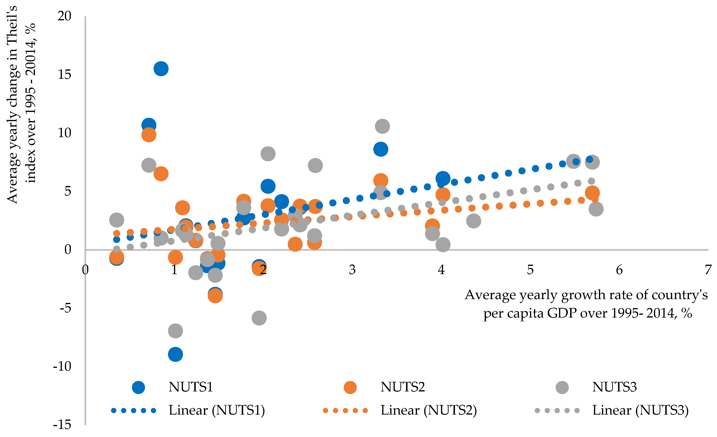
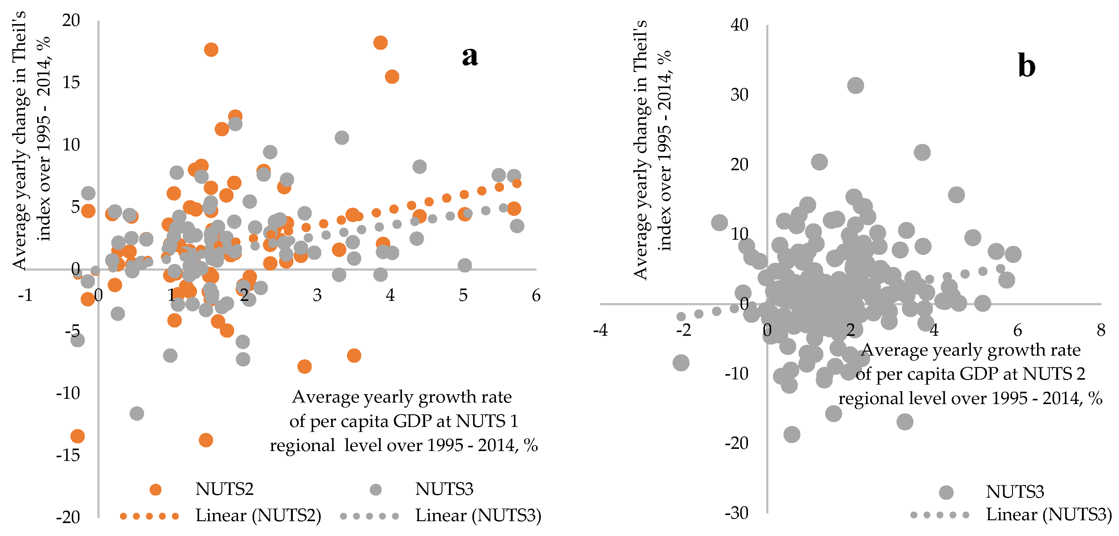
4.4. The Nexus between Growth, Sustainability, Innovation/Technology, and Regional Disparities

In this subsection, we make an attempt to find a link between economic growth, sustainability, investment in R&D (as a proxy for innovation and technology development), and evolution of disparities, trying to answer the following questions: (i) whether growth in the EU could be considered as geographically sustainable, inducing convergence among the regions; (ii) whether countries that are recognized as sustainable in the classical sense are experiencing with regard to convergence; (iii) whether innovations and technology being the main growth factors in modern economy and characterized as geographically highly concentrated activities are causing increasing disparities within countries.
We consider geographically sustainable growth as growth that is spatially inclusive and induces regional convergence. In the case of geographically sustainable growth, we should observe negative correlation between economic growth and evolution of within-country disparities (i.e., growth should correspond to diminishing spatial inequality). Figure 5 displays nexus between growth and evolution of within-country disparities at different regional levels.
Instead of being negative, the correlation between countries’ economic growth and evolution of within-country disparities is positive, meaning that economic growth is accompanied by divergence (see also Figure A1 in Appendix D for unaveraged growth rates). This is true regardless of region level considered. Estimated correlation coefficient between countries’ per capita GDP growth rate and change in regional inequality at the NUTS 1 and 2 level is similar at about 0.21 and is much higher at NUTS 3 level—0.41. This is evidence that growth is less spatially sustainable at a smaller scale, and territorial differences are more noticeable when smaller regions are considered. Figure 6 displays relationship between growth in NUTS 1 and NUTS 2 level regions and evolution of their within-region disparities.
The analysis of correlation between growth and evolution of disparities at smaller-than-country extent reveals quite the same situation—faster growth at NUTS 1 and 2 level regions correspond to faster growth of within-region disparities—that is, a region’s economic growth and a region’s within-divergence are complementary (see also Figure A2 and Figure A3 in Appendix D for unaveraged growth rates). Estimated correlation at the NUTS 1 regional level is 0.26 (in the case of disparities at the NUTS 2 level) and 0.30 (in the case of disparities at the NUTS 3 level), and 0.18 at the NUTS 2 level (for disparities at the NUTS 3 level).
To examine the relationship between countries’ sustainability and evolution of their within-country disparities, we used Environmental Performance Index (EPI on http://archive.epi.yale.edu/) and Global Sustainable Competitiveness Index (GSCI on http://solability.com/solability/sustainability-publications/the-global-sustainable-competitiveness-index-2). EPI is calculated on the basis of 24 performance indicators across 10 issue categories, and it reveals a tension between two fundamental dimensions of sustainable development: (1) environmental health (which rises with economic growth and prosperity) and (2) ecosystem vitality (which comes under strain from industrialization and urbanization). GSCI reveals the ability of a country to meet the needs and basic requirements of current generations while sustaining or growing the national and individual wealth into the future without depleting natural and social capital. This index is built and calculated based on the sustainable competitiveness model that covers 106 data indicators grouped in 5 pillars: Natural Capital, Social Capital, Resource Management, Intellectual Capital, and Governance Efficiency. Both indices allow measurement of sustainable performance at the aggregate level and none of them account for spatial inequality, thus enabling analysis of whether countries that are recognized as more sustainable in the classical sense were also able to reduce within disparities. Figure 7 displays relationship between countries’ sustainability scores in 2014 and change in disparities over a 20-year period. It was not possible to examine relationships at a smaller (i.e., regional) level, because indices are estimated only at country level.
The relationship between countries’ sustainability and evolution of within-country disparities analysis using both sustainability indices is similar. We observe negative correlation, which implies that relatively more sustainable countries reduced within-country disparities more than less sustainable ones over the analyzed 20-year period (see also Figure A4 and Figure A5 in Appendix D for unaveraged growth rates). In the case of EPI, this negative correlation is true for all regional levels; in the case of GSCI, it is true for NUTS 1 and 2 levels. It seems that sustainability in the classical sense is somehow related to more spatially sustainable growth. It could be partly due to the fact that, nowadays, sustainability indices account for a lot of aspects, for example, governance efficiency, equality, capability to generate wealth, creation of new jobs, and so on, that are very important in promoting regional convergence as well.
The development of innovations and technology, share of hi-tech industries, and knowledge-intensive service sectors are also a part of current sustainability indices. However, these activities, which are spatially clustered by nature due to special needs for infrastructure and human capital, could be positively correlated with spatial inequality. The emergence of new industries driven by new innovations and technologies is the source for new jobs, which are usually created in urban territories that are able to supply necessary infrastructure and human capital. Spatial agglomerations with a large city (usually a capital city) in its core and internationally recognized universities are suppliers of new ideas, as well as a labor force that is capable of converting them into products and business. These agglomerations work as a magnet, attracting young people from lagging regions by providing better study and job opportunities and feeding their growth at the expense of other regions. Investments in R&D could be used as a proxy for measuring how intensively innovations and technologies are developing in countries and regions. Estimated correlation between R&D and evolution of spatial inequalities could shed some light on the externality of innovations and technologies that is not usually kept in mind while assessing their overall impact. Figure 8 displays the relationship between average growth rate of expenditures on R&D at the country level and change in disparities over the 20-year period (see also Figure A6 in Appendix D for unaveraged growth rates).
Estimated correlation between per capita R&D expenditures and within-country disparities is positive, implying that countries with faster growth of investment in innovations and technologies were experiencing faster growth of within-country disparities over the same period. This positive correlation is observed at all regional levels with a slightly different strength—0.23 at NUTS 1, 0.33 at NUTS 2, and 0.29 at NUTS 3 level.
Estimations of this relationship at smaller territorial scale revealed the same picture (see Figure 9 as well as Figure A7 and Figure A8 in Appendix D). NUTS 1 and 2 regions that were characterized by faster growth per capita expenditures on R&D were experiencing relatively faster growth of within-region disparities. Evidence observed at the country and regional levels are in line with our initial statement that investment in R&D (which leads to development of innovations and technologies, which in turn leads to faster economic growth) could be a cause of increasing within-country disparities due to spatially concentrated nature of high-tech industries and knowledge-intensive sectors.
Our estimated relationships between the development of innovations and technology, sustainability, and evolution of within-country disparities are not universal and could be affected by variables that were used to proxy these phenomena. Like EPI and GSCI scores are just an approximation of countries’ achieved sustainability level, R&D is telling only one side of the story about the development of innovations and technologies. As a measure of input, it can show a weak correlation with the output—that is, patents. Nevertheless, our analysis allows us to make some general findings:
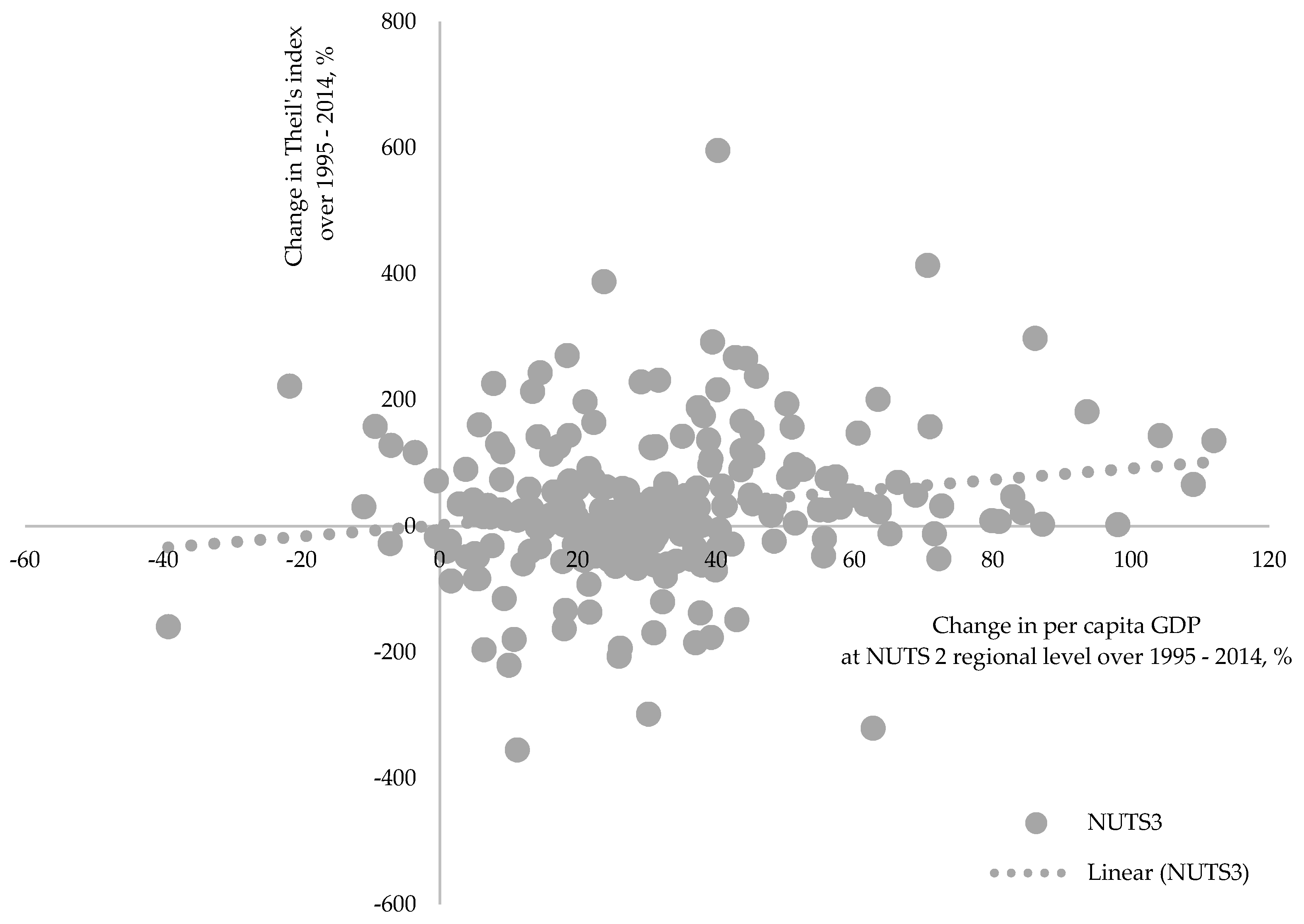
  • Economic growth in the EU is geographically unbalanced, i.e., growth rates in countries and regions positively correlate with the increasing within-country and within-region inequalities, implying that faster growth probably leads to bigger spatial differences.
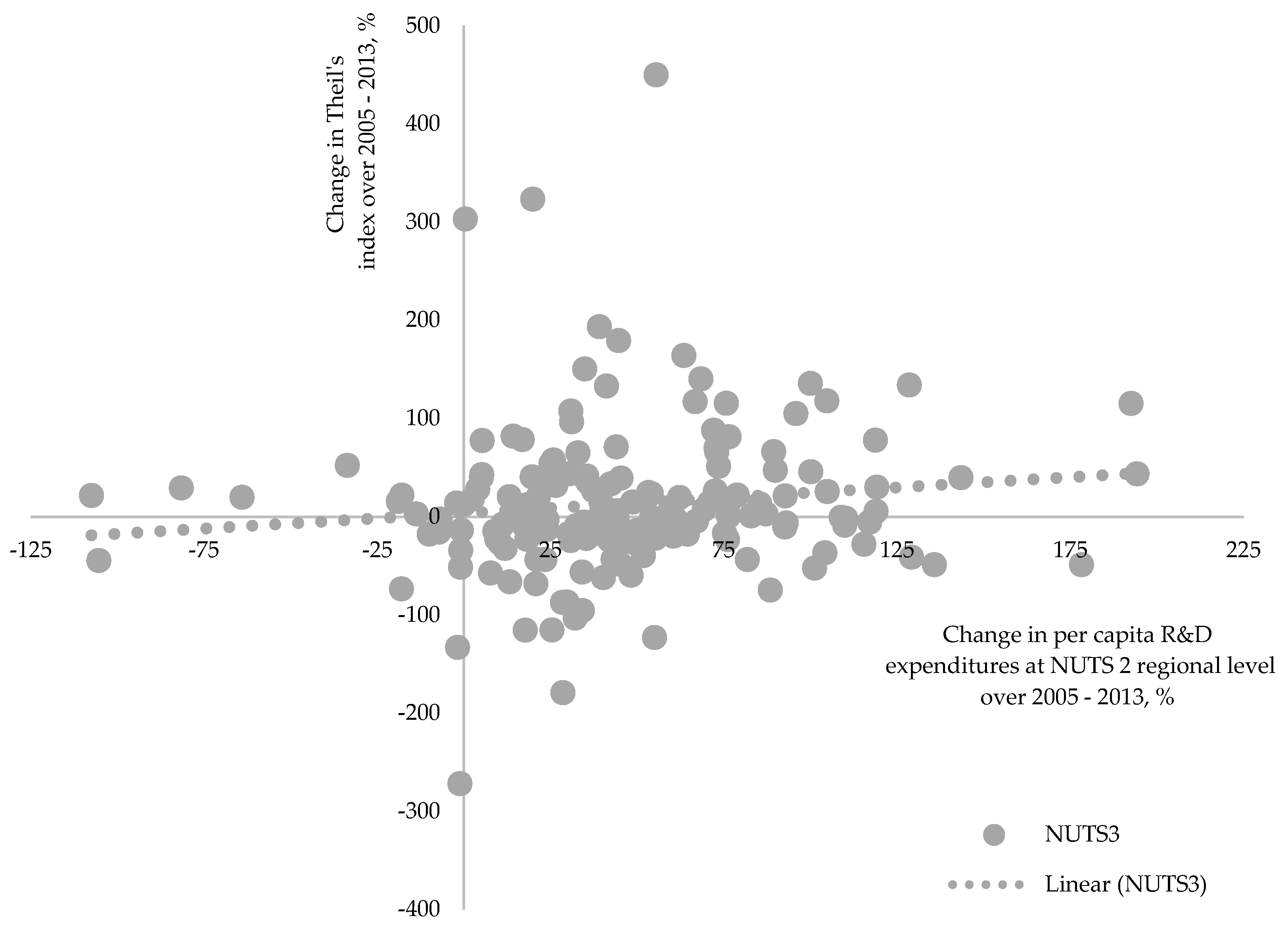
  • The development of innovations and technologies being one of the main growth factors and characterized as spatially concentrated activities could be a potential cause of observed positive correlation between growth and increasing territorial disparities.
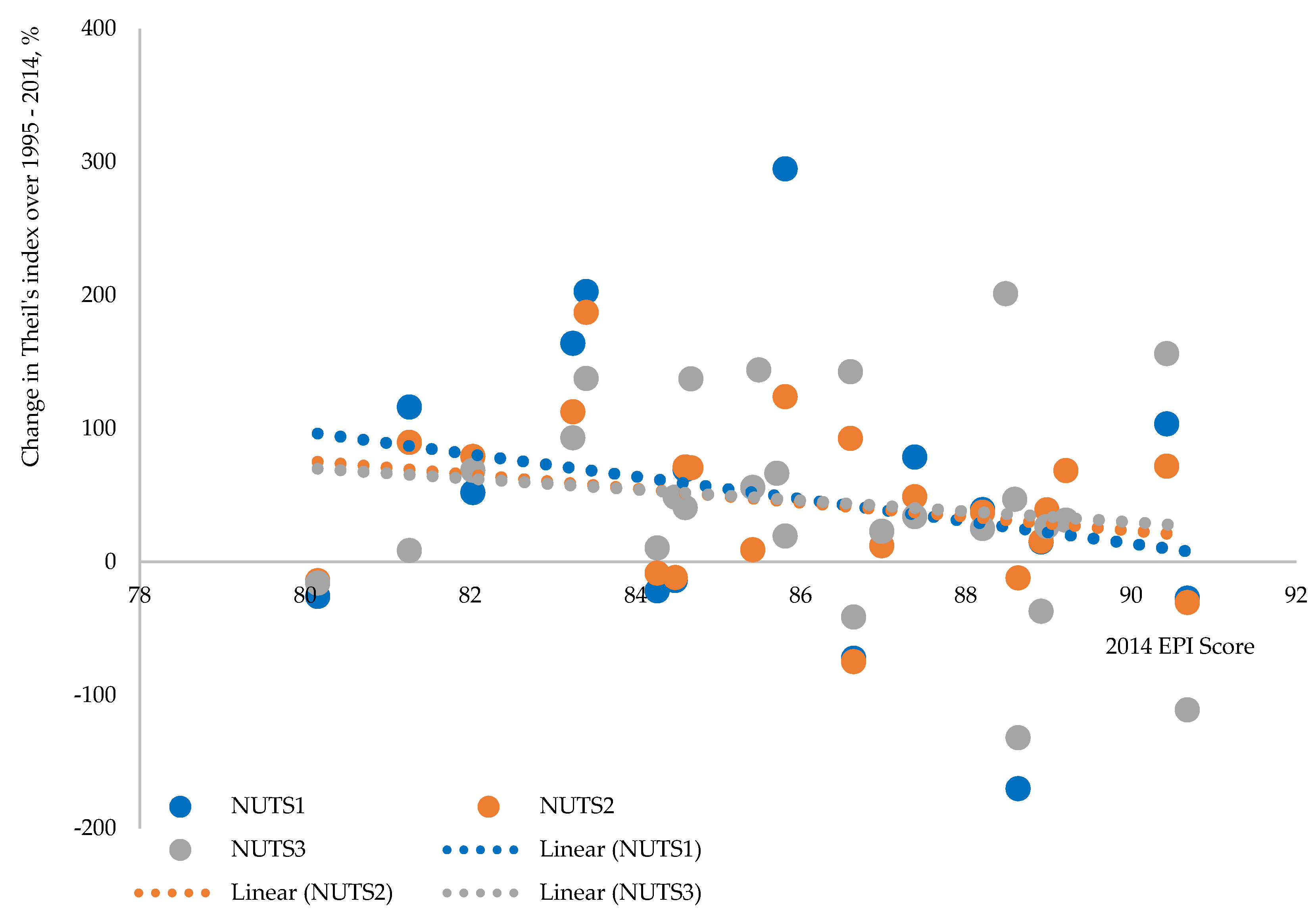
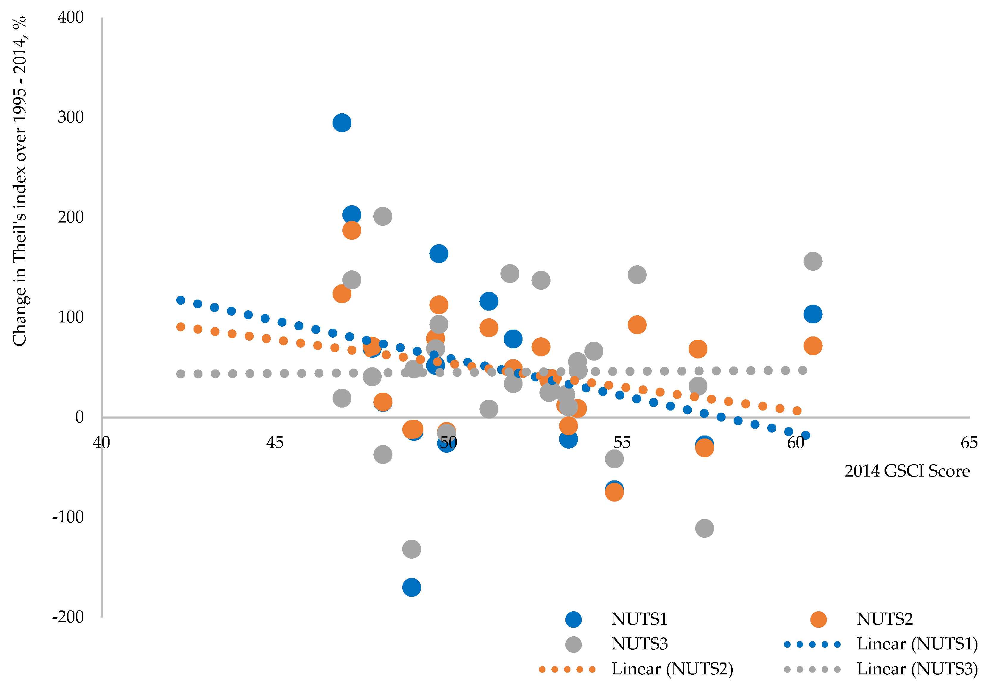
  • Countries’ sustainability is negatively correlated with within-country disparities, implying that actions taken to promote sustainable growth were also in line with promoting more spatially balanced growth.

5. Conclusions

Theoretical analysis shows that there are only several studies covering most EU regions at the NUTS 3 level and no research that includes all NUTS 3 regions. Southern and central eastern European regions are usually analyzed in empirical studies, excluding old members of the EU. The majority of empirical studies have examined convergence/divergence processes by utilizing econometric or statistical models of linear specification. It can be stated that studies confirm convergence in the EU. However, the analysis of convergence at the NUTS 3 level shows that disparities decreased at the EU level but not at national level, and the speed of convergence is not constant over time. The results of empirical studies differ mainly due to the particular method employed, the number of regions observed, and period covered.
Aiming to compare the results of convergence in the EU at different regional levels and to examine evolution of convergence speed, we estimated models of absolute and conditional β-convergence using OLS and WLS. Because detection of β-convergence depends on the estimation of a specific model and due to a number of other limitations of this approach, some researchers promote σ-convergence as more relevant because it deals with a direct measurement of income distribution among regions. In this research, four σ-convergence indices were included—coefficient of variation (CV), Gini coefficient (G), Theil index (T), and mean logarithmic deviation (MLD)—because they use different weighting schemes across the distribution. For each of these measures, disparities in the EU were evaluated at country, NUTS 1, NUTS 2, and NUTS 3 levels in terms of their per capita GDP, with territories being weighted by their population share. The Theil index—a particular case of the generalized entropy index with coefficient 1, which gives equal weights across the distribution—is of special interest in our research because it has a property which is referred to as “decomposability”. Disparities in the EU at the NUTS 3 level were decomposed into (i) between countries (alternatively—between NUTS 1 regions), (ii) within country (alternatively—within NUTS 1 region) at NUTS 2 level, and (iii) within NUTS 2 region at NUTS 3 level components.
The research results of examining absolute and conditional β-convergence in the EU show that convergence in the EU is still present at different regional levels, but its speed is slowing down and during the 2010–2014 period it was already less than 1%, except for the convergence among countries. The smaller the regional units analyzed, the slower the speed of convergence estimated. Convergence between more similar regions is faster, which contradicts the core idea of β-convergence and suggests convergence clubs. Estimated speed of conditional convergence is slightly faster compared to one estimated using the absolute β-convergence model. Urban and capital regions are growing faster, costal and rural regions are lagging. The effect of these factors on growth is mixed over time.
The analysis of four σ-convergence indicators over the 20-year period provided clear evidence that convergence between territories at all levels was just for the period 2000–2009, with rather mixed results for the periods before and after that. The disparities become sharper and convergence less clear as we analyzed smaller territorial unites. For the period when convergence was detected, it was mainly present due to poor territories having become richer; for the period when divergence was detected, it was present not just due to poor regions becoming even poorer but also due to richer regions becoming even richer.
As the decomposition of Theil index shows, the observed decline of regional disparities in the EU as a whole does not necessarily mean that disparities also decline within EU member states. Divergence in the EU during 1995–2000 was present because of increasing within-country disparities, mainly at NUTS 2 level. Disparities in the EU during 2000–2009 were decreasing mainly because of reducing disparities between member states. Convergence in the EU is not present anymore because disparities between countries are stagnating. The part of EU disparities that can be attributed to within-country disparities increased and now account for almost two-fifths of them. In the majority of EU member states, old and new, within-country disparities were growing at all regional levels, thus bringing into question the efficiency of the EU’s Regional Policy.
The analysis of the nexus between growth, sustainability, innovation/technology, and regional disparities shows that economic growth in the EU is spatially unbalanced because growth rates in countries and regions positively correlate with the increasing within-country and within-region disparities. This evidence probably implies that faster growth leads to bigger spatial differences. The development of innovations and technologies, as one of the main growth factors and characterized as spatially concentrated activities, could be a potential cause of observed positive correlation between growth and increasing territorial disparities. We made this conclusion because growth rates of per capita investment in R&D activities at country as well as at region level are positively correlated with growth of within-country and within-region disparities. On the contrary, countries’ sustainability is negatively correlated with within-country disparities, implying that actions taken to promote sustainable growth are also in line with promoting more spatially balanced growth.

Supplementary Materials

The following are available online at https://www.mdpi.com/2071-1050/10/5/1552/s1, Table S1: Sheet W_NUTS1_dis_at_NUTS2, and at NUTS 3 level in Sheet W_NUTS1_dis_at_NUTS3, Table S2: W_Country_dis_at_NUTS1, Table S3: W_Country_dis_at_NUTS2, Table S4: sheet W_Country_dis_at_NUTS3, Table s5: W_NUTS2_dis_at_NUTS3.

Author Contributions

M.B. conceived and designed the empirical analysis; K.M. carried out a literature review; D.C. and A.M.-S. collected and analyzed the data and performed the econometric analysis. All authors reviewed and edited the manuscript, and read and approved the final manuscript.

Funding

This work is a part of the Researchers’ group project on The assessment Model of Return on the EU Regional Support (AMREUS) that has received funding from the Research Council of Lithuania under agreement No. S-MIP-17-114.

Conflicts of Interest

The authors declare no conflict of interest.

Appendix A. Commonly Used σ-Convergence Indices and Their Properties

The five criteria that make income inequality measure “ideal”:
  • Mean or income scale independence—measure should not be affected by the proportional increase or decrease of per capita GDP in all regions.
  • Population size independence—measure should not be affected by the proportional change in population, ceteris paribus.
  • Symmetry—measure should not be affected by the swap in incomes between the two persons.
  • Pigou-Dalton Transfer sensitivity—the income transfer from rich to poor should reduce inequality measured by the index.
  • Decomposability—it is possible to break down inequality index by dimensions like population groups or income sources or other.
There are several indices used to measure inequality that satisfy all five criteria. The most common among them are the Theil indexes and the mean logarithmic deviation. Both are part of the generalized entropy (GE) inequality measures’ family. The general formula to calculate GE indices is:
GE ( α ) = 1 α ( α 1 ) [ 1 N i = 1 N ( y i y ¯ ) α 1 ]
where y ¯ is the mean income (or per capita GDP) and y i is the income or (or per capita GDP) in the region. GE measures can take values between 0 and ∞. Zero represents a situation of perfect equality and a higher value corresponds to a higher level of inequality. The parameter α (which can take any real value) in the class of GE indices represents the weight assigned to distances between incomes at different parts of the distribution. When α is lower, GE becomes more sensitive to the changes in the lower tail of the distribution. The higher the value α, the more sensitive GE becomes to changes that affect the upper tail. The usual values used for α are 0, 1 and 2. GE(1) is Theil T index. GE(0) is also known as Theil L, but is more commonly referred to as the mean logarithmic deviation (MLD).
Table A1. σ-Convergence indices and their properties.
Full NameShort NameFormulaSatisfaction of the Criteria
Mean IndependencePopulation Size IndependenceSymmetryPigou-Dalton Transfer SensitivityDecomposability
Coefficient of variationCV (1) S D y ¯ , where S D = i = 1 N ( y i y ¯ ) 2 w i and w i is the weight of the region acording to population size++++
Gini coefficientG (1) 1 i = 1 N ( X i X i 1 ) ( y i + y i 1 )
Formally, let xi be a point on the X-axis, and yi a point on the Y-axis.
++++
Theil T index or simply Theil indexT (2) i = 1 N y i y ¯ ln ( y i y ¯ ) w i +++++
Theil L index or simply mean logarithmic deviationMLD (2) i = 1 N ln ( y ¯ y i ) w i +++++
(1) CV and G ranges 0–1; (2) T and MLD ranges 0–∞.

Appendix B. Decomposition of the Theil Index

T(total EU disparities at NUTS 3 level) =
T(total disparities between NUTS 1 regions) + T(total within NUTS 1 disparities at NUTS 2 level) + T(total within NUTS 2 disparities at NUTS 3 level)
There are 1342 NUTS 3 level regions in the EU, each with different GDPpc denoted as yi3. The average GDPpc in the EU is y. There are Ni3 people living in each NUTS 3 region and the total EU population is N. All 1342 NUTS 3 level regions are distributed among 98 NUTS 1 level regions with per capita GDP and population denoted as yi1 and Ni1, respectively. Each NUTS 1 region consists of R2 NUTS 2 level regions. yi2 denotes per capita GDP and Ni2 denotes population at NUTS 2 level. Each NUTS 2 region consists of R3 NUTS 3 level regions with GDPpc denoted as yi3 and population denoted as Ni3. Thus, disparities in the EU at NUTS 3 level can be measured and decomposed using Theil index:
T = i = 1 1342 ( N i 3 N y i 3 y l n ( y i 3 y ) ) = [ T 1 ] + [ i = 1 98 ( N i 1 N T 2 ) ] + [ i = 1 98 ( N i 1 N i = 1 R 2 ( N i 2 N i 1 T 3 ) ) ]
T1 measures disparities between 98 NUTS 1 level regions:
T 1 = i = 1 28 ( N i 1 N y i 1 y l n ( y i 1 y ) )
T2 measures within NUTS 1 disparities at NUTS 2 region level and is calculated for each NUTS 1 region:
T 2 = i = 1 R 2 ( N i 2 N i 1 y i 2 y i 1 l n ( y i 2 y i 1 ) )
T3 measures within NUTS 2 disparities at NUTS 3 region level and is calculated for each NUTS 2 region:
T 3 = i = 1 R 3 ( N i 3 N i 2 y i 3 y i 2 l n ( y i 3 y i 2 ) )

Appendix C. Computation and Estimation Results

Table A2. Estimates of absolute β-convergence between EU member states.
PeriodOLS EstimatesWLS Estimates
NUTS0 n = 28NUTS0 (1) n = 28NUTS0 (2) n = 28
β1·100 (t-Stat)Half-Lifeβ1·100 (t-Stat)Half-Lifeβ1·100 (t-Stat)Half-Life
1995–2014−1.1310 *** (−3.579)60.9−1.1926 *** (−3.026)57.8−1.2515 *** (−5.072)55.0
1995–2004−0.7411 (−1.280) −1.2699 * (−1.856) −0.8422 * (−1.960)
2005–2014−1.3615 *** (−4.222)50.6−1.0962 ** (−2.106)62.9−1.6690 *** (−4.711)41.2
1995–19990.5652 (0.5428) −0.5598 (−0.6001) 0.2804 (0.3427)
2000–2004−2.2152 *** (−4.937)30.9−1.9133 *** (−3.197)35.9−2.3205 *** (−6.456)29.5
2005–2009−1.8856 *** (−6.031)36.4−2.2222 *** (−4.545)30.8−2.6250 *** (−7.764)26.1
2010–2014−1.2476 ** (−2.063)55.2−0.0598 (−0.079) −1.1276 ** (−2.090)61.1
2000–2006−2.2753 *** (−5.294)30.1−1.8528 *** (−3.530)37.1−2.2685 *** (−7.351)30.2
2007–2013−1.1469 *** (−2.837)60.1−0.8392 (−1.266) −1.4296 ** (−3.025)48.1
(1) Weights for the countries are assigned according to their contribution to EU’s real GDP; (2) weights for the countries are assigned according to their population share; *, **, *** indicate statistically significant at the 10%, 5%, and 1% levels, respectively.
Table A3. Estimates of absolute β-convergence in the EU at NUTS 1 regional level.
PeriodOLS EstimatesWLS Estimates
NUTS1 n = 98NUTS1 n = 96 (1)NUTS1 (2) n = 98NUTS1 (3) n = 98
β1·100 (t-Stat)Half-Lifeβ1·100 (t-Stat)Half-Lifeβ1·100 (t-Stat)Half-Lifeβ1·100 (t-Stat)Half-Life
1995–2014−0.9957 *** (−6.615)69.3−1.1354 *** (−7.744)60.7−0.8992 *** (−4.317)76.7−1.0647 *** (−7.255)64.8
1995–2004−0.6580 ** (−2.622)105.0−0.9103 *** (−3.859)75.8−1.0130 *** (−2.976)68.1−0.6933 *** (−2.986)99.6
2005–2014−1.2757 *** (−6.398)54.0−1.3661 *** (−6.430)50.4−0.6915 *** (−2.637)99.9−1.3807 *** (−6.895)49.9
1995–19990.4141 (0.9090) −0.0741 (−0.1831) −0.3768 (−0.8123) 0.3392 (0.8121)
2000–2004−2.0894 *** (−9.629)32.8−2.2117 *** (−9.651)31.0−1.7274 *** (−5.812)39.8−2.1336 *** (−10.64)32.1
2005–2009−1.9637 *** (−8.527)35.0−2.1537 *** (−8.928)31.8−1.5998 *** (−5.432)43.0−2.2098 *** (−9.381)31.0
2010–2014−0.9494 *** (−3.166)72.7−0.9434 *** (−2.906)73.10.0523 0.1505 −0.9333 *** (−3.370)73.9
2000–2006−2.0790 *** (−10.45)33.0−2.2070 *** (−10.55)31.1−1.7034 *** (−6.477)40.3−2.1040 *** (−11.58)32.6
2007–2013−0.9806 *** (−3.763)70.3−0.9918 *** (−3.511)69.5−0.4105 (−1.270) −1.1446 *** (−4.579)60.2
(1) Top one percentile and bottom one percentile of regions according to their real per capita GDP are excluded from the sample; (2) weights for the regions are assigned according to their contribution to EU’s real GDP; (3) weights for the regions are assigned according to their population share; *, **, *** indicate statistically significant at the 10%, 5%, and 1% levels, respectively.
Table A4. OLS estimates of conditional β-convergence in the EU at NUTS1 regional level.
Periodβ1·100 (t-Stat)Half-LifeR-SquaredDummies
Capital (1)Country
1995–2014−0.9957 *** (−6.615)69.30.313
1995–2014−0.955 *** (−6.958)72.30.4380.9455 *** (4.584)
1995–2014−0.4370 (−1.627) 0.9000.6541 *** (4.259)27 country dummies (2)
1995–2004−0.6580 ** (−2.622)105.00.067
1995–2004−0.5962 ** (−2.554)115.90.2051.4241 *** (4.059)
1995–2004−0.1155 (−0.2729) 0.8780.7671 *** (3.171)27 country dummies (2)
2005–2014−1.2757 *** (−6.298)54.00.299
2005–2014−1.2908 *** (−6.546)53.40.3230.5137 * (1.823)
2005–2014−0.5570 ** (−2.117)124.10.9330.4554 *** (2.746)27 country dummies (2)
1995–19990.4141 (0.9090) 0.009
1995–19990.4638 (1.026) 0.0371.1456 * (1.685)
1995–19990.2346 (0.3596) 0.9070.4460 (1.196)27 country dummies (2)
2000–2004−2.0894 *** (−9.629)32.80.491
2000–2004−2.0827 *** (−10.23)32.90.5561.2013 *** (3.736)
2000–2004−0.9063 * (−1.992) 0.8940.1093 (0.3763)27 country dummies (2)
2005–2009−1.9637 *** (−8.527)35.00.431
2005–2009−1.9894 *** (−8.918)34.50.4730.8731 *** (2.739)
2005–2009−1.2438 *** (−2.715)55.40.8761.2708 *** (4.402)27 country dummies (2)
2010–2014−0.9494 *** (−3.166)72.70.095
2010–2014−0.9681 *** (−3.219)71.30.1030.3760 (0.9396)
2010–2014−0.2248 (−0.5962) 0.914−0.1433 (−0.5964)27 country dummies (2)
2000–2006−2.0790 *** (−10.45)33.00.532
2000–2006−2.0712 *** (−11.64)33.10.6301.4045 *** (5.000)
2000–2006−0.9933 ** (−2.368)69.40.9020.3705 (1.384)27 country dummies (2)
2007–2013−0.9806 *** (−3.763)70.30.129
2007–2013−0.9800 *** (−3.732)70.40.129−0.0121 (−0.03384)
2007–2013−0.5108 (−1.515) 0.9150.3080 (1.448)27 country dummies (2)
(1) Coefficient’s estimate is multiplied by 100; (2) Germany is set as a benchmark country; *, **, *** indicate statistically significant at the 10%, 5%, and 1% levels, respectively.
Table A5. Estimates of absolute β-convergence in the EU at NUTS 2 regional level.
PeriodOLS EstimatesWLS Estimates
NUTS2 n = 276NUTS2 n = 270 (1)NUTS2 (2) n = 276NUTS2 (3) n = 276
β1·100 (t-Stat)Half-Lifeβ1·100 (t-Stat)Half-Lifeβ1·100 (t-Stat)Half-Lifeβ1·100 (t-Stat)Half-Life
1995–2014−0.7910 *** (−8.2072)87.3−0.9832 *** (−10.48)70.1−0.6963 *** (−5.653)99.2−0.9993 *** (−11.11)69.0
1995–2004−0.4319 *** (−2.6909)160.1−0.7389 *** (−4.854)93.5−0.8957 *** (−4.537)77.0−0.6582 *** (−4.544)105.0
2005–2014−1.0978 *** (−8.3578)62.8−1.2489 *** (−8.860)55.2−0.4328 *** (−2.798)159.8−1.3110 *** (−10.88)52.5
1995–19990.8794 *** (2.9251) 0.1550 (0.6151) −0.1470 (−0.5463) 0.4268 1.617
2000–2004−1.8170 *** (−13.6779)37.8−1.8980 *** (−13.23)36.2−1.5115 *** (−8.516)45.5−2.0335 *** (−16.22)33.7
2005–2009−1.7763 *** (−11.5163)38.7−2.0465 *** (−12.55)33.5−1.1304 *** (−6.058)61.0−2.0938 *** (−14.17)32.8
2010–2014−0.7705 *** (−4.2016)89.6−0.8309 *** (−4.133)83.10.1335 (0.6748) −0.9569 *** (−5.810)72.1
2000–2006−1.7255 *** (−14.5624)39.8−1.8320 *** (−14.41)37.5−1.4220 *** (−8.977)48.4−1.9319 *** (−17.10)35.5
2007–2013−0.8345 *** (−4.9769)82.7−0.9122 *** (−4.964)75.6−0.1706 (−0.9200) −1.0483 *** (−7.034)65.8
(1) Top one percentile and bottom one percentile of regions according to their real per capita GDP are excluded from the sample; (2) weights for the regions are assigned according to their contribution to EU’s real GDP; (3) weights of the regions are assigned according to their population share; *, **, *** indicate statistically significant at the 10%, 5% and 1% levels, respectively.
Table A6. OLS estimates of conditional beta convergence in the EU at NUTS2 regional level.
Periodβ1·100 (t-Stat)Half-LifeR-SquaredDummies
Capital (1)Country
1995–2014−0.7910 *** (−8.207)87.30.197
1995–2014−0.8247 *** (−9.226)83.70.3141.2244 *** (6.822)
1995–2014−0.4727 *** (−3.201)146.30.8120.8089 *** (6.309)27 country dummies (2)
1995–2004−0.4319 *** (−2.691)160.10.026
1995–2004−0.4809 *** (−3.167)143.80.1341.7808 *** (5.841)
1995–2004−0.7601 *** (−3.168)90.80.7831.2475 *** (5.988)27 country dummies (2)
2005–2014−1.0978 *** (−8.358)62.80.203
2005–2014−1.1511 *** (−8.767)59.90.2240.7021 *** (2.722)
2005–2014−0.2330 (−1.272) 0.8390.2800 * (1.661)27 country dummies (2)
1995–19990.8794 *** (2.925) 0.030
1995–19990.8352 *** (2.805) 0.0551.6074 *** (2.689)
1995–1999−0.0585 (−0.1582) 0.8541.2376 *** (3.857)27 country dummies (2)
2000–2004−1.8170 *** (−13.68)37.80.406
2000–2004−1.8865 *** (−14.75)36.40.4571.3911 *** (5.094)
2000–2004−1.1656 *** (−4.530)59.10.7930.3065 (1.276)27 country dummies (2)
2005–2009−1.7763 *** (−11.52)38.70.326
2005–2009−1.8583 *** (−12.17)37.00.3571.0793 *** (3.598)
2005–2009−0.7200 ** (−2.448)95.90.7450.9690 *** (3.579)27 country dummies (2)
2010–2014−0.7705 *** (−4.202)89.60.061
2010–2014−0.8219 *** (−4.430)84.00.0700.5627 (1.636)
2010–2014−0.0163 (−0.06718) 0.808−0.2634 (−1.161)27 country dummies (2)
2000–2006−1.7255 *** (−14.56)39.80.436
2000–2006−1.8052 *** (−16.33)38.00.5171.5936 *** (6.754)
2000–2006−1.0763 *** (−4.581)64.10.7940.5728 *** (2.611)27 country dummies (2)
2007–2013−0.8345 *** (−4.977)82.70.083
2007–2013−0.8580 *** (−5.041)80.40.0850.2653 (0.8207)
2007–2013−0.1461 (−0.6570) 0.8210.1787 (0.8693)27 country dummies (2)
(1) Coefficient’s estimate is multiplied by 100; (2) Germany is set as a benchmark country; *, **, *** indicate statistically significant at the 10%, 5%, and 1% levels, respectively.
Table A7. Estimates of absolute β-convergence in the EU at NUTS 3 regional level.
PeriodOLSWLS
NUTS3 n = 1342NUTS3 n = 1313 (1)NUTS3 (2) n = 1342NUTS3 (3) n = 1342
β1·100 (t-Stat)Half-Lifeβ1·100 (t-Stat)Half-Lifeβ1·100 (t-Stat)Half-Lifeβ1·100 (t-Stat)Half-Life
1995–2014−0.7388 *** (−16.1096)93.5−0.9547 *** (−21.69)72.2−0.4734 *** (−8.401)146.1−0.9227 *** (−21.14)74.8
1995–2004−0.6240 *** (−7.8956)110.7−0.9710 *** (−12.74)71.0−0.6090 *** (−6.810)113.5−0.6161 *** (−8.827)112.2
2005–2014−0.8983 *** (−13.9355)76.8−1.0673 *** (−15.38)64.6−0.2652 *** (−3.935)261.0−1.2020 *** (−20.74)57.3
1995–19990.5871 *** (4.2287) −0.0765 (−0.6088) −0.0129 (−0.09915) 0.3316 *** (2.639)
2000–2004−2.0118 *** (−26.7588)34.1−2.1140 *** (−26.18)32.4−1.2175 *** (−14.31)56.6−1.9431 *** (−28.74)35.3
2005–2009−1.5947 *** (−18.9970)43.1−1.8466 *** (−20.48)37.2−0.8071 *** (−8.817)85.5−1.8865 *** (23.97)36.4
2010–2014−0.5614 *** (−6.4016)123.1−0.6658 *** (−6.948)103.80.0895 (1.051) −0.9075 *** (−11.31)76.0
2000–2006−1.7042 *** (−28.3455)40.3−1.8387 *** (−28.72)37.3−1.1112 *** (−15.02)62.0−1.7704 *** (−30.80)38.8
2007–2013−0.7085 *** (−8.4738)97.5−0.8196 *** (−8.985)84.2−0.8130 (−0.9887) −1.0079 *** (−13.80)68.4
(1) Top one percentile and bottom one percentile of regions according to their real per capita GDP are excluded from the sample; (2) weights for the regions are assigned according to their contribution to EU’s real GDP; (3) weights of the regions are assigned according to their population share; *, **, *** indicate statistically significant at the 10%, 5%, and 1% levels, respectively.
Table A8. OLS estimates of conditional β-convergence in the EU at NUTS 3 regional level.
Periodβ1·100 (t-Stat)Half-LiveR-SquaredDummies
Capital (2)Coastal (2)Rural–Urban Typology (1)
Urban (2)Rural (2)Country
1995–2014−0.7388 *** (−16.1096)93.50.162
1995–2014−0.83252 *** (−18.0820)82.90.2330.9929 *** (6.6366)−0.2617 *** (−4.1637)0.3189 *** (4.0480)−0.1640 ** (−2.3458)
1995–2014−0.4660 *** (−6.3317)148.40.6660.9846 *** (9.1502)−0.0194 (−0.3728)0.0987 * (1.7345)−0.0461 (−0.9306)27 country dummies (3)
1995–2004−0.6240 *** (−7.896)110.70.044
1995–2004−0.8097 *** (−10.46)85.30.1661.7922 *** (7.128)0.8244 *** (7.805)0.8148 *** (6.154)0.2497 ** (2.126)
1995–2004−0.6834 *** (−5.476)101.10.6311.2522 *** (6.862)0.0766 (0.8654)0.3866 *** (4.008)−0.0783 (−0.9318)27 country dummies (3)
2005–2014−0.8983 *** (−13.94)76.80.127
2005–2014−0.8551 *** (−13.65)80.70.2800.2706 (1.391)−1.3167 *** (−16.09)−0.0967 (−0.9421)−0.4982 *** (−5.517)
2005–2014−0.3244 *** (−3.679213.30.7160.7574 *** (5.620)−0.1402 ** (−2.179)−0.1752 ** (−2.482)0.0361 (0.5899)27 country dummies (3)
1995–19990.5871 *** (4.229) 0.013
1995–19990.4708 *** (3.277) 0.0401.2508 *** (2.679)0.7578 *** (3.864)0.6788 *** (2.761)0.3943 * (1.808)
1995–1999−0.2849 (−1.458)243.00.6971.2068 *** (4.223)−0.0712 (−0.5137)0.1571 (1.040)−0.0337 (−0.2556)27 country dummies (3)
2000–2004−2.0118 *** (−26.76)34.10.348
2000–2004−2.1498 *** (−27.86)31.90.3921.3516 *** (5.155)0.6563 *** (5.951)0.5275 *** (3.812)0.3412 *** (2.795)
2000–2004−0.9112 *** (−6.046)75.70.6110.0933 (0.4031)0.1384 (1.252)0.2349 * (1.940)0.0175 (0.1660)27 country dummies (3)
2005–2009−1.5947 *** (−19.00)43.10.212
2005–2009−1.6371 *** (−18.95)42.00.2720.9641 *** (3.595)−0.9952 *** (−8.819)−0.0646 (−0.4563)−0.5350 *** (−4.296)
2005–2009−0.7911 *** (−5.251)87.30.5591.2484 *** (5.421)0.1198 (1.090)−0.0155 (−0.1286)−0.1778 * (−1.700)27 country dummies (3)
2010–2014−0.5614 *** (−6.402)123.10.030
2010–2014−0.5547 *** (−6.265)124.60.134−7.41 *10−5 (−0.028)−1.3676 *** (−12.39)0.0490 (0.3528)−0.3830 *** (−3.120)
2010–2014−0.2912 ** (−2.237)237.70.5890.4422 ** (2.192)−0.2974 *** (−3.114)−0.2695 ** (−2.577)0.1486 (1.634)27 country dummies (3)
2000–2006−1.7042 *** (−28.35)40.30.375
2000–2006−1.8246 *** (−29.37)37.60.4091.3487 *** (6.391)0.3090 *** (3.481)0.2684 ** (2.410)0.0431 (0.4387)
2000–2006−0.6343 *** (−5.330)108.90.6360.3081 * (1.685)0.1074 (1.230)0.1100 (1.151)−0.1374 * (−1.655)27 country dummies (3)
2007–2013−0.7085 *** (−8.474)97.50.051
2007–2013−0.6316 *** (−7.717)109.40.207−0.1609 (−0.6505)−1.6141 *** (−15.54)−0.1611 (−1.235)−0.5818 *** (−5.063)
2007–2013−0.5392 *** (−4.748)128.20.6750.8833 *** (5.047)−0.1021 (−1.225)−0.2491 *** (−2.727)0.1439 * (1.813)27 country dummies (3)
(1) Intermediate is set as a benchmark type; (2) coefficient’s estimate is multiplied by 100; (3) Germany is set as a benchmark country; *, **, *** indicate statistically significant at the 10%, 5%, and 1% levels, respectively.
Table A9. Indices of σ-convergence.
Index/Regional Level/Year19951996199719981999200020012002200320042005200620072008200920102011201220132014
Coefficient of variationNUTS 30.6120.6160.6190.6200.6350.6340.6330.6260.6200.6170.6240.6170.6240.6190.6270.6370.6400.6440.6510.663
NUTS 20.5300.5310.5310.5310.5370.5370.5340.5280.5220.5180.5200.5140.5170.5120.5120.5180.5210.5250.5290.536
NUTS 10.4920.4910.4880.4870.4890.4950.4910.4860.4780.4730.4710.4650.4630.4570.4510.4550.4570.4590.4610.463
EU 280.4340.4330.4300.4280.4280.4300.4270.4210.4160.4120.4100.4070.4020.3910.3840.3850.3880.3910.3910.391
Gini coefficient, %NUTS 321.821.922.022.122.222.922.822.421.921.521.420.920.620.320.320.320.019.819.819.8
NUTS 221.521.421.321.221.221.621.521.020.319.919.619.118.918.518.418.618.618.418.418.4
NUTS 121.621.421.321.221.221.521.120.620.019.419.118.518.418.117.818.018.118.118.018.1
EU 2818.417.817.317.016.516.015.715.014.213.713.212.912.512.512.112.912.612.812.912.6
Theil indexNUTS 30.2130.2160.2170.2180.2210.2260.2220.2140.2050.1980.1950.1880.1830.1760.1730.1760.1750.1740.1730.171
NUTS 20.1910.1930.1940.1940.1970.2010.1970.1880.1800.1730.1690.1620.1570.1500.1470.1490.1490.1470.1460.144
NUTS 10.1800.1830.1820.1840.1830.1890.1840.1760.1680.1610.1560.1490.1440.1360.1330.1350.1340.1330.1310.130
EU 280.1620.1650.1640.1640.1630.1660.1620.1530.1460.1390.1330.1280.1210.1130.1090.1100.1090.1080.1060.104
Mean logarithmic deviationNUTS 30.1740.1760.1760.1760.1810.1830.1810.1770.1710.1680.1670.1630.1620.1580.1570.1610.1610.1620.1630.164
NUTS 20.1490.1490.1490.1490.1500.1520.1500.1460.1410.1370.1360.1320.1310.1270.1250.1280.1280.1280.1290.129
NUTS 10.1370.1370.1360.1360.1360.1390.1370.1330.1280.1240.1220.1180.1150.1110.1090.1100.1110.1110.1110.111
EU 280.1160.1160.1150.1140.1140.1150.1130.1090.1050.1020.0990.0960.0930.0880.0850.0850.0860.0860.0860.085
Table A10. Decomposition of Theil index into between-country disparities, within-country disparities at NUTS2 level, and within-NUTS 2 disparities at NUTS 3 level components.
Theil Index/Year19951996199719981999200020012002200320042005200620072008200920102011201220132014
Total Theil index0.2130.2160.2160.2180.2190.2260.2210.2140.2050.1980.1950.1880.1830.1760.1730.1760.1750.1740.1730.171
Between-country disparitiesTheil index0.1630.1640.1640.1640.1630.1660.1610.1530.1460.1390.1330.1270.120.1120.1080.1090.1080.1080.1060.104
% of total76.476.075.675.174.373.372.971.671.170.168.467.565.663.562.561.961.961.961.260.4
Within-country disparities at NUTS 2 levelTheil index0.0290.030.030.0310.0330.0350.0350.0350.0340.0340.0360.0350.0370.0390.0390.040.0410.040.040.041
% of total13.413.714.014.315.115.715.816.516.717.318.418.820.221.922.322.823.222.923.423.8
Within-NUTS 2 disparities at NUTS 3 levelTheil index0.0220.0220.0230.0230.0230.0250.0250.0250.0250.0250.0260.0260.0260.0260.0260.0270.0260.0260.0270.027
% of total10.210.310.410.610.611.011.311.912.212.613.213.814.214.515.215.215.015.115.415.8
Table A11. Decomposition of Theil index into between-NUTS 1 disparities, within-NUTS 1 disparities at NUTS2 level, and within-NUTS 2 disparities at NUTS 3 level components.
Theil Index/Year19951996199719981999200020012002200320042005200620072008200920102011201220132014
Total Theil index0.2130.2160.2160.2180.2190.2260.2210.2140.2050.1980.1950.1880.1830.1760.1730.1760.1750.1740.1730.171
Between-NUTS 1 disparitiesTheil index0.1810.1830.1830.1830.1840.1890.1840.1760.1680.1610.1560.1490.1440.1360.1330.1350.1340.1330.1310.130
% of total85.184.884.584.283.983.683.382.481.981.380.179.478.477.676.676.576.676.576.075.6
Within-NUTS 1 disparities at NUTS 2 levelTheil index0.0100.0110.0110.0110.0120.0120.0120.0120.0120.0120.0130.0130.0140.0140.0140.0150.0150.0150.0150.015
% of total4.84.95.15.25.55.45.55.75.96.26.76.97.47.98.28.38.48.48.68.6
Within-NUTS 2 disparities at NUTS 3 levelTheil index0.0220.0220.0230.0230.0230.0250.0250.0250.0250.0250.0260.0260.0260.0260.0260.0270.0260.0260.0270.027
% of total10.210.310.410.610.611.011.311.912.212.613.213.814.214.515.215.215.015.115.415.8

Appendix D

Figure A1. Nexus between growth and evolution of within-country disparities at different regional levels.
Sustainability 10 01552 g0a1
Figure A2. Nexus between growth of regional per capita GDP and evolution of within-NUTS 1 disparities at NUTS 2 and 3 levels.
Sustainability 10 01552 g0a2
Figure A3. Nexus between growth of regional per capita GDP and evolution of within-NUTS 2 disparities at NUTS 3 level.
Sustainability 10 01552 g0a3
Figure A4. Nexus between countries’ Environmental Performance Index (EPI) score and change of within-region disparities at different regional levels.
Sustainability 10 01552 g0a4
Figure A5. Nexus between countries’ Global Sustainable Competitiveness Index (GSCI) score and change of within-region disparities at different regional levels.
Sustainability 10 01552 g0a5
Figure A6. Relationship between expenditures on R&D and evolution of spatial disparities within the country.
Sustainability 10 01552 g0a6
Figure A7. Relationship between expenditures on R&D and evolution of spatial disparities within the NUTS 1 regions.
Sustainability 10 01552 g0a7
Figure A8. Relationship between expenditures on R&D and evolution of spatial disparities within the NUTS 2 regions.
Sustainability 10 01552 g0a8

References

  1. Arbia, G.; Basile, R.; Salvatore, M. Measuring spatial effects in parametric and non-parametric modelling of regional growth and convergence. In UNU/WIDER Project Meeting on Spatial Inequality in Development; UNU/WIDER: Helsinki, Finland, 2003. [Google Scholar]
  2. Braga, V. Regional growth and local convergence: Evidence for Portugal. In Proceedings of the 43rd Congress of the European Regional Science Association: “Peripheries, Centres, and Spatial Development in the New Europe”, Jyväskylä, Finland, 27–30 August 2003; pp. 1–19. [Google Scholar]
  3. Soukiazis, E.; Antunes, M. The evolution of real disparities in Portugal among the NUTS III regions. An empirical analysis based on the convergence approach. Estudos Reg. 2004, 6, 163–181. [Google Scholar]
  4. Artelaris, P.; Kallioras, D.; Petrakos, G. Regional Inequalities and Convergence Clubs in the European Union New Member-States. Dis. Paper Ser. Univ. Thessaly 2010, 16, 43–62. [Google Scholar]
  5. Cardoso, C.; Pentecost, E.J. Regional Growth and Convergence: The Role of Human Capital in Portuguese Regions. Work. Pap. Loughborough Univ. 2011, 3, 1–28. [Google Scholar]
  6. Supińska, J. Does human factor matter for economic growth? Determinants of economic growth process in CEE countries in light of spatial theory. Bank i Kredyt 2013, 44, 505–532. [Google Scholar]
  7. Viegas, M.; Antunes, M. Convergence in the Spanish and Portuguese NUTS 3 regions: An exploratory spatial approach. Intereconomics 2013, 48, 59–66. [Google Scholar] [CrossRef] [Green Version]
  8. Tsionas, M.; Sakkas, S.; Baltas, N.C. Regional Convergence in Greece (1995–2005): A Dynamic Panel Perspective. Econ. Res. Int. 2014. [Google Scholar] [CrossRef]
  9. Panzera, D.; Postiglione, P. Economic growth in Italian NUTS 3 provinces. Ann. Reg. Sci. 2014, 53, 273–293. [Google Scholar] [CrossRef]
  10. Lopes, J.C.; Araújo, T. Geographic and Demographic Determinants of Regional Growth and Convergence: A Network Approach. Revista Portuguesa de Estudos Reg. 2016, 43, 1–15. [Google Scholar]
  11. Folfas, P. Income Absolute Beta-Convergence of NUTS 3 Level Regions in New EU Member States before and During a Crisis. Folia Oecon. Stetin. 2016, 16, 151–162. [Google Scholar] [CrossRef]
  12. Hegerty, S.W. Regional Convergence and Growth Clusters in Central and Eastern Europe: An Examination of Sectoral-Level Data. Eastern Eur. Bus. Econ. J. 2016, 2, 95–110. [Google Scholar]
  13. Regional Growth and Convergence of the NUTS 3 Regions of Eastern European Countries. Available online: http://www.fiwi.uni-bayreuth.de/de/download/WPs/WP_13-03.pdf 2017 (accessed on 7 May 2018).
  14. Geppert, K.; Stephan, A. Regional disparities in the European Union: Convergence and agglomeration. Pap. Regional Sci. 2008, 87, 193–217. [Google Scholar] [CrossRef]
  15. Paas, T.; Kuusk, A.; Schlitte, F.; Võrk, A. Econometric Analysis of Income Convergence in Selected EU Countries and Their Nuts 3 Level Regions 2007; University of Tartu: Tartu, Estonia, 2004. [Google Scholar]
  16. Paas, T.; Schlitte, F. Regional Income Disparities and Spatial Interaction of Regional Convergence Processes. In Recent Development in INFORUM-Type Modelling; Wyd; Plich, M., Przybyliński, M., Eds.; Łόdź University Press: Łόdź, Poland, 2008. [Google Scholar]
  17. Mikulić, D.; Lovrinčević, Ž.; Nagyszombaty, A.G. Regional convergence in the European Union, new Member States and Croatia. South East European J. Econ. Bus. 2013, 8, 7–19. [Google Scholar] [CrossRef]
  18. Kramar, H. Regional convergence and economic development in the EU: The relation between national growth and regional disparities within the old and the new member states. Int. J. Latest Trends Finance Econ. Sci. 2016, 6, 1052–1062. [Google Scholar]
  19. Goecke, H.; Hüther, M. Regional convergence in Europe. Intereconomics 2016, 51, 165–171. [Google Scholar] [CrossRef]
  20. Solow, R.M. A Contribution to the Theory of Economic Growth. Q. J. Econ. 1956, 70, 65–94. [Google Scholar] [CrossRef]
  21. Koopmans, T. On the Concept of Optimal Economic Growth. In The Econometric Approach to Development Planning; Koopmans, T., Ed.; Rand McNally: Chicago, IL, USA, 1965; pp. 225–300. [Google Scholar]
  22. Barro, R.J.; Sala-i-Martin, X. Convergence across States and Regions. Brookings Pap. Econ. Activity 1991, 1, 107–182. [Google Scholar] [CrossRef]
  23. Barro, R.J.; Sala-i-Martin, X. Convergence. J. Political Econ. 1992, 100, 223–251. [Google Scholar] [CrossRef] [Green Version]
  24. Fagerberg, J.; Verspagen, B. Heading for Divergence? Regional Growth in Europe Reconsidered. J. Common Mark. Stud. 1996, 34, 431–448. [Google Scholar] [CrossRef]
  25. Fingleton, B. Economic Geography with Spatial Econometrics. A ‘Third Way’ to Analyse Economic Development and ‘Equilibrium’ with Application to the EU Regions; Economics Working Papers eco99/21; European University Institute: San Domenico di Fiesole, Florence, Italy, 1999. [Google Scholar]
  26. Cuadrado-Roura, J.R. Regional Convergence in the European Union. From Hypothesis to the Actual Trends. Ann. Reg. Sci. 2001, 35, 333–356. [Google Scholar] [CrossRef]
  27. Cappelen, A.; Castellacci, F.; Fagerberg, J.; Verspagen, B. The Impact of EU Regional Support on Growth and Convergence in the European Union. J. Common Mark. Stud. 2003, 41, 621–644. [Google Scholar] [CrossRef]
  28. Cappelen, A.; Castellacci, F.; Fagerberg, J.; Verspagen, B. Regional Disparities in Income and Unemployment in Europe. In European Regional Growth. Advances in Spatial Science 2003; Fingleton, B., Ed.; Springer: Berlin/Heidelberg, Germany, 2003. [Google Scholar] [CrossRef]
  29. Baumont, B.; Ertur, C.; Le Gallo, J. Spatial Convergence Clubs and the European Regional Growth Process, 1980–1995. In European Reg. Growth; Fingleton, B., Ed.; Springer Verlag: Berlin, Germany, 2003; pp. 131–158. [Google Scholar]
  30. Carrington, A. A Divided Europe? Regional Convergence and Neighbourhood Spillover Effects. Kyklos 2003, 56, 381–394. [Google Scholar] [CrossRef]
  31. Bräuninger, M.; Niebuh, A. Agglomeration, Spatial Interaction and Convergence in the EU; HWWA Discussion Paper 322; Hamburg Institute of International Economics: Hamburg, Germany, 2005. [Google Scholar] [CrossRef]
  32. Próchniak, M.; Witkowski, B. Time stability of the beta convergence among EU countries: Bayesian model averaging perspective. Econ. Modell. 2013, 30, 322–333. [Google Scholar] [CrossRef]
  33. Campos, N.F.; Coricelli, F.; Moretti, L. Economic Growth and Political Integration: Estimating the Benefits from Membership in the European Union Using the Synthetic Counterfactuals Method. IZA Discussion Paper 8162. 2014. Available online: https://ssrn.com/abstract=2432446 (accessed on 03 May 2018).
  34. Goedemé, T.; Collado, D. The EU Convergence Machine at Work. To the Benefit of the EU’s Poorest Citizens? J. Common Mark. Stud. 2016, 54, 1142–1158. [Google Scholar] [CrossRef]
  35. Magrini, S. The Evolution of Income Disparities among the Regions of the European Union. Reg. Sci. Urban Econ. 1999, 29, 257–281. [Google Scholar] [CrossRef]
  36. Fingleton, B. Estimates of Time to Economic Convergence. An Analysis of Regions of the European Union. Int. Reg. Sci. Rev. 1999, 22, 5–34. [Google Scholar] [CrossRef]
  37. Rodríguez-Pose, A.; Crescenzi, R. Research and development, spillovers, innovation systems, and the genesis of regional growth in Europe. Reg. Stud. 2008, 42, 51–67. [Google Scholar] [CrossRef] [Green Version]
  38. Kim, B.W. Growth regression revisited: R&D promotes convergence? Appl. Econ. 2012, 44, 1347–1362. [Google Scholar] [CrossRef]
  39. Rego, C.; Caleiro, A. On the Spatial Diffusion of Knowledge by Universities Located in Small and Medium Sized Towns. iBusiness 2010, 2, 99–105. [Google Scholar] [CrossRef]
  40. Rego, C.; da Saudade Baltazar, M.; Caleiro, A. Higher education and social cohesion. Higher Educ. Soc. Sci. 2012, 2, 17–24. [Google Scholar]
  41. Guerreiro, G.; Guerreiro, A. Regional Convergence and R&D Investment: Applied investigation in Portugal. In Proceedings of the 55th Congress of the European Regional Science Association: “World Renaissance: Changing roles for people and places”, Lisbon, Portugal, 25–28 August 2015; Available online: http://hdl.handle.net/10419/124652 (accessed on 10 March 2018).
  42. Furková, A.; Chocholatá, M. Interregional R&D spillovers and regional convergence: A spatial econometric evidence from the EU regions. Equilibrium. Quarterly J. Econ. Econ. Policy 2017, 12, 9–24. [Google Scholar] [CrossRef]
  43. Barro, R.J.; Sala-i-Martin, X. Economic Growth, 2nd ed.; The MIT Press: Cambridge, MA, USA, 2004. [Google Scholar]
  44. Boldrin, L.; Canova, F. Inequality and Convergence in Europe’s Regions. Reconsid. Eur. Reg. Policies Econ. Policy 2001, 16, 207–253. [Google Scholar] [CrossRef]
  45. Yin, L.; Zestos, G.K.; Michelis, L. Economic Convergence in the European Union. J. Econ. Integr. 2003, 18, 188–213. [Google Scholar] [CrossRef]
  46. Neven, D.J. Regional Convergence in the European Union. J. Common Mark. Stud. 1995, 33, 47–65. [Google Scholar] [CrossRef]
  47. López-Bazo, E.; Vayá, E.; Mora, A.J.; Suriñach, J. Regional economic dynamics and convergence in the European Union. Ann. Reg. Sci. 1999, 33, 343–370. [Google Scholar] [CrossRef]
  48. Tondl, G. Convergence after Divergence: Regional Growth in Europe; Springer: Wien, Austria; New York, NY, USA, 2001; ISBNs 9783211836729, 3211836721. [Google Scholar]
  49. Basile, R.; de Nardis, S.; Girardi, A. Regional Inequalities and Cohesion Policies in the European Union; ISAE Working Paper, 23; Italian National Institute of Statistics: Rome, Italy, 2005. [CrossRef]
  50. Baumol, W. Productivity Growth, Convergence and Welfare: What the Long-Run Data Show? Am. Econ. Rev. 1986, 76, 1072–1085. Available online: http://www.jstor.org/stable/1816469 (accessed on 10 March 2018).
  51. Durlauf, S.N.; Johnson, P.A. Multiple regimes and cross-country growth behaviour. J. Appl. Econ. 1995, 10, 365–384. [Google Scholar] [CrossRef]
  52. Galor, O. Convergence? Inferences from theoretical models. Econ. J. 1996, 1056–1069. [Google Scholar] [CrossRef]
  53. Borsi, M.T.; Metiu, N. The evolution of economic convergence in the European Union. Empir. Econ. 2015, 48, 657–681. [Google Scholar] [CrossRef]
  54. von Lyncker, K.; Thoennessen, R. Regional club convergence in the EU: Evidence from a panel data analysis. Empir. Econ. 2017, 52, 525–553. [Google Scholar] [CrossRef]
  55. Bourdin, S. National and regional trajectories of convergence and economic integration in Central and Eastern Europe. Can. J. Reg. Sci. 2015, 38, 55–63. [Google Scholar]
  56. Ferrer, E.M. Regional Convergence and Productive Structure in Iberian Regions: A Spatial Approach. Revista Portuguesa de Estudos Regionais 2018, 47, 5–20. [Google Scholar]
  57. Gagliardi, L.; Percoco, M. The impact of European Cohesion Policy in urban and rural regions. Reg. Stud. 2017, 51, 857–868. [Google Scholar] [CrossRef]
  58. Paas, T.; Kuusk, A.; Schlitte, F. Modelling Regional Income Convergence in EU-25; Regional and Urban Modeling 283600067; University of Tartu: Tartu, Estonia, 2004. [Google Scholar]
  59. Percoco, M. Impact of European Cohesion Policy on regional growth: Does local economic structure matter? Reg. Stud. 2017, 51, 833–843. [Google Scholar] [CrossRef]
  60. Smetkowski, M.; Wójcik, P. Regional Convergence in Central and Eastern European Countries: A Multidimensional Approach. Eur. Plan. Stud. 2012, 20, 923–939. [Google Scholar] [CrossRef]
Figure 1. Absolute β-convergence between EU member states and NUTS 1 regions over 1995–2014. (a) Convergence between member states and (b) Convergence between NUTS 1 regions.
Sustainability 10 01552 g001
Figure 2. Absolute β-convergence in the EU at NUTS 2 and 3 regional levels over 1995–2014. (a) Convergence between NUTS 2 regions and (b) Convergence between NUTS 3 regions.
Sustainability 10 01552 g002
Figure 3. Indices of σ-convergence in the EU at different regional levels over 1995–2014. (a) Coefficient of variation; (b) Gini coefficient; (c) Mean Logarithmic Deviation and (d) Theil index.
Sustainability 10 01552 g003
Figure 4. Decomposition of EU disparities over 1995–2014, using Theil index.
Sustainability 10 01552 g004
Figure 5. Nexus between growth and evolution of within-country disparities at different regional levels.
Sustainability 10 01552 g005
Figure 6. Nexus between growth of regional per capita GDP and evolution of within-NUTS 1 and 2 disparities at different levels. (a) Nexus between growth and evolution of within-NUTS 1 disparities and (b) Nexus between growth and evolution of within-NUTS 2 disparities
Sustainability 10 01552 g006
Figure 7. Nexus between countries’ sustainability and change of within-country disparities at different regional levels. (a) Countries’ sustainability is estimated using EPI score and (b) Countries’ sustainability is estimated using GSCI score
Sustainability 10 01552 g007
Figure 8. Nexus between expenditures on R&D and evolution of spatial disparities within the country.
Sustainability 10 01552 g008
Figure 9. Nexus between expenditures on R&D and evolution of within-NUTS 1 and 2 disparities at different levels. (a) Nexus between R&D and evolution of within-NUTS 1 disparities and (b) Nexus between R&D and evolution of within-NUTS 2 disparities
Sustainability 10 01552 g009
Table 1. Summary of empirical studies of convergence in the EU at NUTS 3 level.
ResearchAnalysis PeriodMethodResearch SampleResult
Arbia et al. [1]1951–2000σ-convergence (coefficient of variation);
β-convergence estimated using common cross-sectional ordinary least squares (OLS) approach;
Moran’s I for spatial autocorrelation
92 Italian regionsSpillover and convergence clubs are spatially concentrated
Artelaris et al. [4]1990–2005σ-convergence (coefficient of variation)Regions of EU New Member StatesRegional convergence clubs were identified in many of the new EU member states
Bourdin [55]1995–2007Gini indexRegions of Central and Eastern Europe (CEE)Convergence was identified at a national level but regional inequalities within each country were increasing
Braga [2]1970–2001β-convergence estimated using nonlinear least squares and Levenberg–Marquardt methodPortuguese regionsThe growth and convergence within regions and between regions is influenced by clustering phenomenon
Cardoso, Pentecost [5]1991–2008β-convergence via shift-share analysis was applied, which allows the decomposition of the deviation of a region’s output growth ratePortuguese regionsSignificant and positive impact of human capital on regional growth and convergence was identified
Ferrer [56]2000–2005Moran’s I for spatial autocorrelation; spatial Durbin model (SDM); spatial autoregressive model (SAR), spatial error model (SEM)82 Iberian regionsIberian regions grew at a cumulative growth rate of 0.303%, while in the Spanish and Portuguese regions it increased at 0.313% and 0.03%, respectively.
Folfas [11]2000–2011β-convergence (spatial lagged model (SLM) and spatial error model (SEM))211 regions of CEEAbsolute β-convergence was not confirmed during the crisis of 2008–2011
Gagliardi, Percoco [57]2000–2006Regression discontinuity design RDD and a local average treatment effect (LATE) estimator1233 EU-25 regionsEuropean Cohesion funds positively affected the growth of lagging rural regions
Goecke, Hüther [19]2000–2011σ-convergence (coefficient of variation)1289 European regionsHigh starting level of GDP per capita does indeed correlate with a growth rate in this variable below the EU average
Hegerty [12]2000–2013Moran’s I for spatial autocorrelation238 regions of CEEConvergence is more likely to occur at the national level than the regional level
Kotosz, Lengyel [13]2000–2014σ-convergence;
β-convergence estimated using cross-sectional approach
99 regions in Eastern Europeβ-convergence cannot be proved
Kramar [18]2000–2011σ-convergence (coefficient of variation)EU-28 1090 regionsDisparities between growing economic centers and lagging rural areas are increasing, but there is no clear evidence that the degree of divergence is higher in the fastest growing countries
Lopes, Araújo [10]1995–2012Stochastic geometry81 Portuguese and Spanish regionsVery low velocities of convergence
Mikulić et al. [17]2001–2008β-convergence estimated using common cross-sectional OLS approachEU-27 and CroatiaAbsolute β-convergence occurs at the national level for EU countries and for NMS regions
Paas et al. [15]1995–2002β-convergence estimated using cross-sectional approach;
σ-convergence (coefficient of variation)
1214 EU 25 regionsOld and new member states are experiencing significant regional disparities
Paas et al. [58]1995–2002β-convergence (OLS; spatial lagged model (SLM); spatial error model (SEM))EU-25 countriesThe EU-15 and the new member states (NMS) experienced absolute regional income convergence during the EU pre-enlargement period
Panzera, Postiglione [9]1981–2008Spatial Durbin Model;
Bayesian Interpolation Method
103 Italian regionsDifferent growth paths appear to confirm the presence of disparities among the Italian provinces
Percoco [59]1997–2008.Heterogeneous local average treatment effects (HLATE) estimation procedure based on an RDD and a local average treatment effect (LATE) estimatorEU-25 countriesEconomic disparities are decreasing while promoting the service sector at its early stages
Schlitte, Paas [16]1995–2003σ-convergence (coefficient of variation);
β-convergence estimated using common cross-sectional OLS approach;
Moran’s I for spatial autocorrelation
861 regions of the EURegional catching-up process was relatively slow
Smetkowski, Wójcik [60]1998–2005σ-convergence (coefficient of variation);
Kernel density estimator (KDE); Moran’s I for spatial autocorrelation
179 CEE regionsWeak regional convergence was identified
Soukiazis, Antunes [3]1991–2000β-convergence estimated using OLS estimation by pooling the data, least squares dummy variable (LSDV) estimation assuming that regional specific effects are fixed and the generalized least squares (GLS) estimation assuming that regional differences are random30 Portuguese regionsConvergence is more conditional than absolute
Stephan et al. [14]1980–2000Analysis of distribution (Kernel estimation, Markov chain analysis);
β-convergence estimated using cross-sectional approach
167 regions in the EU-15 except the eastern part of GermanyDisparities between the countries are decreasing
Supińska [6]1999–2008β-convergence (spatial lagged model (SLM) and spatial error model (SEM))211 CEE regionsSpatial coefficients occurred to be significant and positive
Tsionas et al. [8]1995–2005Generalized method of moments (GMM) estimation of Barro regressions in dynamic panel data framework13 Greek regions and 51 prefecturesConvergence is identified at the NUTS 3 level, while between NUTS 2 regions it was not detected
Viegas, Antunes, [7]1995–2008σ-convergence (coefficient of variation);
Moran’s I for spatial autocorrelation
75 Portuguese and Spanish regionsResults point to a σ-divergence process between 1995 and 2008, while at the national level, both countries have followed a sigma convergence process during the same period
Table 2. Evolution of within-country disparities measured using Theil index at different regional levels.
Country CodeNUTS 1 Level (1)NUTS 2 Level (2)NUTS 3 Level (3)
Number of RegionsDisparities among Regions Increased (I) or Decreased (D)Number of RegionsDisparities among Regions Increased (I) or Decreased (D)Number of RegionsDisparities among Regions Increased (I) or Decreased (D)
1995–20141995–20002000–20092009–20141995–20141995–20002000–20092009–20141995–20141995–20002000–20092009–2014
BE3DIDD11DIDD44DDDI
BG2IIID6IIID28IIII
CZ1 8IIID14IIII
DK1 5IIII11IDII
DE16DIDD38DIDD402IIDD
EE1 1 5IIID
IE1 2IIDI8IIII
EL4IIII13IIII52IDII
ES7IIDI19IIDI59DIDI
FR9IIII27IIII101IIDI
HR1 2IIII21IDII
IT5DDDI21DDDI110IIID
CY1 1 1
LV1 1 6IIDI
LT1 1 10IIID
LU1 1 1
HU3IIID7IIID20IIID
MT1 1 2IDII
NL4IIDD12IIII40IIII
AT3DDDD9DDDD35DIDD
PL6IIII16IIII72IDID
PT3DDDI7DIDD25DDDD
RO4IIID8IIII42IIII
SI1 2IDID12IIID
SK1 4IIID8IIDI
FI2DDID5DDID19DDDD
SE3IIID8IIID21IIDI
UK12IIDI40IIII173IIID
Tot.98DIDD276DIDD1342DIDD
(1) Raw data is provided in Excel file ‘Supplementary material’ sheet W_Country_dis_at_NUTS1; (2) raw data is provided in Excel file ‘Supplementary material’ sheet W_Country_dis_at_NUTS2; (3) raw data is provided in Excel file ‘Supplementary material’ sheet W_Country_dis_at_NUTS3.

