1. Introduction
This paper studies the mathematical structure introduced in [
1] and used in a deep way in [
2] to provide an algebraic framework for an abstract notion of embodiment in Neuroscience by means of multigraphs. Its aim is to examine the presence and extent of homology in a certain multilayer structure inherited from multigraphs, that is, graphs that we allow to have parallel edges between the same vertices. For this purpose, we need to translate many of the concepts defined in the references above to the language of simplicial complexes [
3]. Along these lines, we hope to show that the concepts of Topological Data Analysis help to give clarity to the formal models of Neuroscience [
4].
The structure considered entails dynamical behavior, which needs a suitable setting to be studied. In the present paper, we try to understand which geometric features are preserved along this dynamism. For this purpose, a way to combine multigraphs is defined by obtaining larger and larger networks, that is, the role of the operator ⊙. Our idea here is to investigate how much the complex structure changes due to the process of merging graphs, in particular to try to know to what extent some features are preserved as the dimension of the complex grows through several applications of ⊙.
As a general idea, we obviate the classical interaction of a static multilayer network containing graphs (as in [
5]). Instead, we focus on its underlying algebraic structure: how it changes the whole network and what remains the same in it. It is precisely through the interaction among graphs using ⊙ that we obtain a sequence of configurations that allows us to observe these remaining features.
These sequences are called filtrations in the context of a simplicial complex (see, for example, [
6]). One of the main contributions of this work is to make interact simplices rather than graphs. That is, we construct simplicial complexes out of graphs and make ⊙ to act on the simplices obtained by the graphs in the multilayer network. However, rather than considering the usual concept of filtration, we introduce the concept that we call interaction filtration, which is nothing more than the sequence of configurations obtained by successive use of our operator ⊙.
It is precisely with the aim of obtaining new applications in Neuroscience that new mathematical ideas are developed that fit with our purpose. In this paper, we introduce the construction of multicomplexes out of multigraphs. Multicomplexes were nicely defined in [
7], where many algebraic considerations were made starting from simple graphs rather than multigraphs. Making use of multigraphs, however, we are able to endow the multicomplexes with much more interesting structures and extend their potential applications.
Moreover, the graphs being here used have the particularity that they are coloured on the edges. This is a particularity just mentioned in [
7] but necessary for the purpose mentioned of formalizing the structure of networks for which the colours relate to different layers. All these features (multigraphs plus colours) make the multicomplexes richer in their potentiality to generate useful formalizations for concrete examples.
Once the structure of a simplicial complex is presented, we investigate usual concepts such as persistent homology and the Betti numbers [
3] to figure out the shape of the network through time. These measures, belonging to the field of Topological Data Analysis, have not been investigated in the context of multicomplexes, to the knowledge of the author, and are addressed in the last pages of this paper. Our contribution here consists of an extension of the incremental algorithm given in [
3]. The formulae found in that reference, allowing the calculation of the Betti numbers of a series of simplicial configurations in a filtration, are extended in Proposition 10 to cover the case of multicomplexes.
As a general purpose, we introduce throughout this paper as many pictures as possible to facilitate the understanding of the content. On the other hand, the concepts used in the second section, mainly belonging to Lattice Theory, are to be seen as a mathematical foundation of the structure developed further in the following sections.
The main contributions of this article are as follows: 1. the definition of the operation of merging coloured multicomplexes, together with a new idea of filtration for them, and 2. a way to calculate Betti numbers in this context (Proposition 10).
We outline this paper as follows. In
Section 2, we introduce the main concepts and present the inspiring example. The crucial idea of ordering is defined and some results emerging from the lattice structure it gives rise to are proved.
Section 3 is devoted to deeply explaining how multicomplexes can be defined out of multigraphs and how are they merged through the operator ⊙ working now on simplices. Some categorical considerations are made for the structure [
8]. A new idea of filtration,
interaction filtration, is defined in
Section 4, closely related to the graphs obtained by the application of ⊙. This suggests the use of homology in the following section by introducing the idea of many-dimensional holes.
Section 5 contains a way to calculate Betti numbers for the structure defined as an extension of the known incremental method, an algorithm defined in [
6].
2. An Ordered Set of Multigraphs
Let
X be a set; a multisubset is a pair
, where
Y is the underlying subset of
X and
is the multiplicity function that assigns to each element in
Y the number of occurrences (see [
9]). Further definitions can be found in [
1], which are based on [
8,
10], where multilayer networks are included in an abstraction called the network model.
Definition 1. A multigraph G on a set of nodes is a multisubset of edges that corresponds to pairs of elements of , together with the multiplicity function .
Similarly, the edges could have different colors. Let C be a finite set of colors, and a mapping that assigns to each edge a subset of colors. We will consider a coloured multigraph as the pair and, for , we say that a multigraph is k-colored if is onto and , i.e., k denotes the number of colors included in the multigraph. We define the set of nodes indexed by the set and denote by the set of coloured multigraphs with such n nodes. Let c be a single colour; then, we denote by the set of 1-colored layers. Every multigraph is from now on a coloured multigraph.
2.1. Chains of Graphs out of ⊗ and ⊙
Let
be a set of colours; then, we define the set of multilayer networks as the product
Then, every multigraph in is called a -coloured multilayer. We can also have sets of multilayers in the form , as shown in the following example.
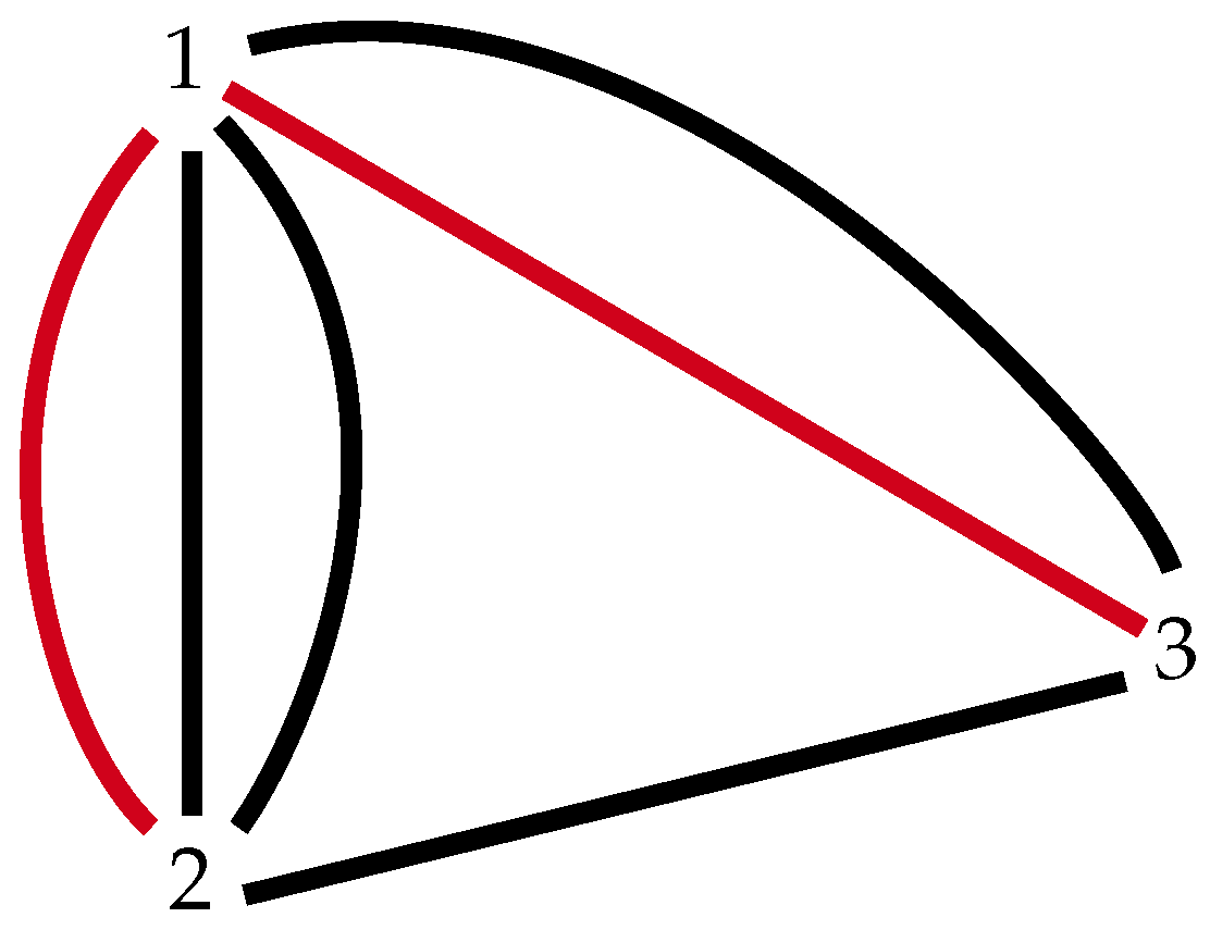
Example 1. A multilayer built out of layers and can be represented as Figure 1.
The tensor product ⊗ places layers in parallel, establishing a determined order (i.e., is not the same as ). This operation is non-commutative and imposes a first multilayer order configuration. To simplify notation, we fix nodes into the finite set V and denote such a set by (without reference to n).
Now, we are in position to define a commutative binary operation in . Let us denote by ⊔ the disjoint union of sets.
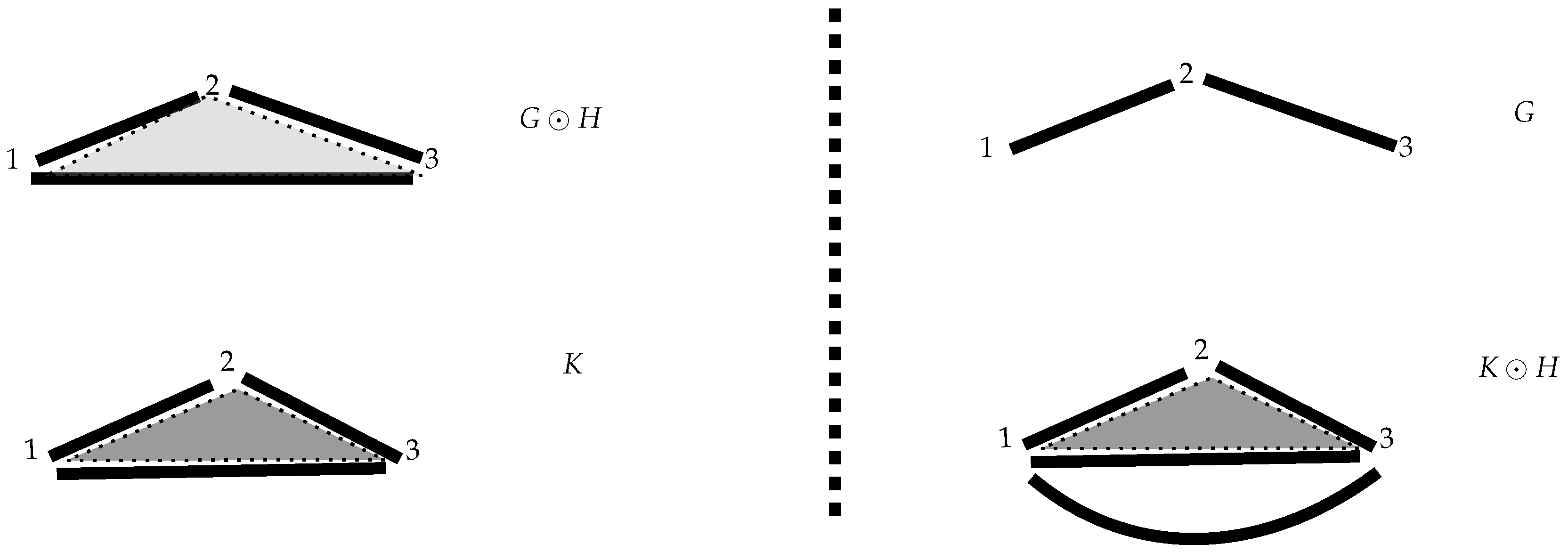
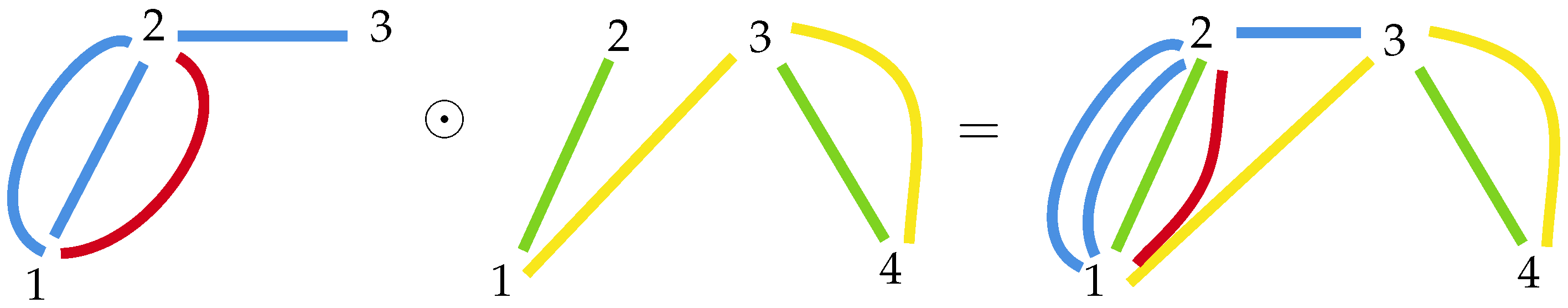
Definition 2. Let C and V be fixed sets of colors and nodes, respectively. Let a k-colored multigraph and a j-colored multigraph , and assume that , and . Then, the operationproduces a new ()-colored multigraph , where with vertices, where defined as , , and , where the mappings are defined in a natural way. Example 2. For and . Figure 2. It is seen that ⊙ is a commutative operation while ⊗ is not. We establish ⊙ having priority over ⊗, that is,
Notice that we have defined two different ways of composing multigraphs: ⊗ and ⊙. Also note that, with this notation, the tensor means no interaction between multigraphs; they are just interpreted as put together. That is, we have sets of concatenations in the form
with
for
.
By abusing the notation, we denote by the set of all chains in the above form constructed out of a fixed set of monochrome multigraphs .
Example 3. For , we have the concatenations However, and in order to simplify the notation, we sometimes use lowercase letters as multigraphs and fix the number of colours as k; that is, when no other parameter is stated.
For the sake of clarity, we include a table containing the basics of the notation defined so far (
Table 1).
2.2. Embodiment and Composition
In this section, we show the main example of the application of the mathematical content of this paper (see [
2] for more details).
From the formal concepts above, we now introduce the biological and experiential interpretations, followed by formal ways to compound the colours of different layers into multilayers. This is given by the operation ⊙, which formalizes the complexity of brain–body interactions and the irreductive nature of conscious experience.
Considering an ideal example, layers act as continuous biological membranes. Some of these layers might correspond to specific neural networks, while others might account for bodily systems, such as the metabolic system, cholinergic system and immune system, among others.
The elements inside layers (nodes) represent biological processes, cells, neurons and/or their assemblies, e.g., brain regions and organs such as the gut, liver, heart, lungs, etc. (
Figure 3A). In [
11], these systems were thought of as functional, anatomical and metabolic membranes of brain–body organization, acting and reacting as an independent living system (e.g., two amoebas interacting).
Regarding conscious experience, layers create an identity through their agency and convey several isolated or minimal sets of possible experiences. In
Figure 3A, for schematic purposes, we associate each colour aspect with one sense, such as layers accounting for internal (organs) and external (sense) minimal unimodal experiences. Each layer by itself is a closed unity, and the experience becomes embodied by intrinsic internal/external layer definition.
The dynamical composition of these layers also has an impact within the brain, as shown in
Figure 3B.
In this model, the brain and the body admit a meaningful and nontrivial decomposition into living experiential systems (as mathematically shown in the rest of this paper). Remarkably, to give a first mathematical account, we do not need to specify the nature of these nodes and layers. Here, we recognize that a simple and scalable principle is only the interaction between layers.
3. The Partial Ordered Structure
The operation ⊙ defined can be seen as an accumulation of vertices and edges of two given multigraphs. By using ⊙, we obtain a new multigraph with possibly more colors than the original ones.
Given and , we understand that is more complex or is over . Following this intuition, we say by convention that since we consider that is more complex, in some sense, than . Let us formalize this idea.
Definition 3 ([
12]).
A partially ordered set or a poset is a set with a binary operation ≤, which is reflexive, antisymmetric and transitive. Let P be a poset. We say that is a bottom element if for every and is a top element if for every . Now, we define the relation ≤ in by ordering the concatenations of multigraphs as given in the following.
Definition 4. Let π be a permutation of the set with . For every with , we writeif and only if there is no l such that and . Example 4. Observe that![Ijt 02 00007 i001]() whileand
whileand This partial order allows us to define the following mappings.
Definition 5. Let the mapping :for . We say that are comparable through if . By adding as the identity, it is easy to see that are order-preserving. For the sake of clarity, we use the notation for any mapping defined above, avoiding the list of indices. These mappings will be useful in the sequel; the next example illustrates how these functions work and describes, in some sense, a flow on as a poset.
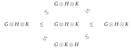
Example 5. For the elements in example 3, we have diagrams![Ijt 02 00007 i002]() as well as
as well as![Ijt 02 00007 i003]()
From the example above, we extract two immediate results. The first one establishes that one can obtain the top element after an action of every over a given concatenation whatever the ordering could be and the second that are increasing.
Lemma 1. for a permutation of .
Proof. Every f converts every symbol ⊗ into a ⊙ in every position of the chains. □
Lemma 2. .
Proof. Whenever an f is acting over the chain, we obtain a greater one according to the definition of the ordering. □
Proposition 1. is a partial ordered set with top .
Proof. Observe that the order of is described by the mappings (see Example 5). Reflexivity is given by while transitivity is immediate by definition of the mappings . For antisymmetry, we recall the form of the ordering given in the previous definition; now, a concatenation can only be compared both ways with another concatenation if they are both the same. In this case, they are compared by means of the same whenever a ⊙ appears in the j-position of the concatenation. □
Notice that we cannot dualize the above, since inverse mappings such as
, for which
lose the well-definedness condition for the non-commutativity of ⊗.
3.1. A Lattice-Ordered Partial Monoid
We saw above that we can define a partial order in a set of multigraphs and showed that this order yields several properties in such a framework. In this section, we go a little further and provide a lattice structure for .
A meet (resp. join) semilattice is a poset
such that any two elements
x and
y have a greatest lower bound (called meet or infimum) (resp. a smallest upper bound (called join or supremum)), denoted by
(resp.
). A poset
is called a lattice and denoted by
if for every pair of elements we can construct into the poset their meet and their join. These definitions can be found for instance, in [
12]. Let us define meet and join operators for the poset
.
Definition 6. Given and (in short, and ), we write for such thatand we write for such that One can easily check the usual properties of both operations. That is, for every : and for every one has . And dually, and for every one has .
Proposition 2. The absorption laws are satisfied for every :
;
.
Proof. Let us prove the first assertion. For
and
, we construct
such that
and
as
which can be expressed as
and becomes the same assignation as that considered for
. □
Recalling that a minimal element in a poset is an element such that it is not greater than any other element in the poset, we have the following.
Proposition 3. is an upper-bounded lattice, where the following hold:
is the top;
are minimal elements for π a permutation of the set .
Proof. Check that , and . □
Proposition 4. is distributive.
Proof. Let
,
and
. Now,
, where
which is exactly the same operator as
for
. □
Proposition 5. Mappings preserve meets and joins.
Proof. Straightforward calculations. □
3.2. Complements
In [
12], a complemented lattice is defined as a bounded lattice (with least element 0 and greatest element 1) in which every element
a has a complement, i.e., an element
b such that
and
. Also, given a lattice
L and
, we say that
is an orthocomplement of
x if the following conditions are satisfied:
A lattice is orthocomplemented if every element has an orthocomplement. We give a slightly different approach.
Definition 7. We say that an upper-bounded lattice with a set of minimal elements is semi-orthocomplemented if every element has a complement, i.e., an element b such that and for a certain .
Proposition 6. is a semi-orthocomplemented lattice.
Proof. For
, consider
, where
□
3.3. Partiality
Now, some concepts from [
13] are taken and adapted for the case of a partial operation such as ours (since not every pair of elements are comparable through ≤).
Definition 8. A system is called a lattice-ordered partial monoid if the following hold:
is a partial monoid;
is a lattice with ∧ and ∨;
implies and ;
;
.
for every .
We introduce a different operation from that considered in [
13]: + will be partial for
. This is the reason to study it as a lattice-ordered partial monoid. Firstly, a partial semigroup structure will be defined for
by defining + as follows:
for
.
Now, we see that + is an associative, commutative and partial operation. It is actually a partial minimum.
Proposition 7. is a partial commutative monoid.
Proof. The operation + satisfies associativity; suppose that
are comparable to each other. Now,
Since is finite, the unique top element (see Proposition 1) is the identity element. □
Let be a partial monoid and let be a mapping. Recall that a partial homomorphism between partial monoids is mapping that preserves the binary operation; namely, , and implies that . A mapping between lattice-ordered partial monoids is a lattice partial homomorphism if it is a partial homomorphism of partial monoids that preserves meets and joins.
Proposition 8. Mappings are partial homomorphisms.
Proof. By virtue of Proposition 5, mappings preserve meets and joins. From the definition of the partial operation +, we know that x and y are comparable if and only if there exists . As is monotone, if , then and and are comparable. So . Finally, as 1 is the top element for every x, . However, for Lemma 2 we have . Therefore, . □
Proposition 9. is a lattice-ordered partial monoid.
Proof. Suppose that
are comparable. Observe that
and
together with the fact that for
,
Note in particular that
equals to
□
4. Multicomplexes out of Multigraphs
In this section, we show how to define multicomplexes out of multigraphs. Our main references for this will be [
6,
7]. The concept of a multicomplex is developed in [
7] for simple graphs, where the complexes are in addition ordered and coloured in their vertices. We will follow the notation and formulation of that paper but will make use of the concepts introduced so far, the operation ⊙ in particular, and will colour the edges rather than the vertices.
4.1. The Clique Complex of a Graph
Let us begin this section by sketching some concepts. A simplicial complex with vertex set V is a non-empty collection of finite subsets of V, called cells, such that it is closed under inclusion. That is, for and , . The dimension of a cell A is and denotes the set of j-cells (cells of dimension j) for . We write them as . The of a simplicial complex are the vertices themselves. The dimension of a simplicial complex is the maximal dimension of a cell in it. For a (j + 1)-cell , its boundary is defined to be the set of j-cells .
With all these concepts, taken from [
7], we construct a simplicial complex in a different way. Recall that a k-clique in a graph
G is a complete subgraph of dimension
.
Definition 9. Given a graph G, its clique complex, denoted by , has the following characteristics:
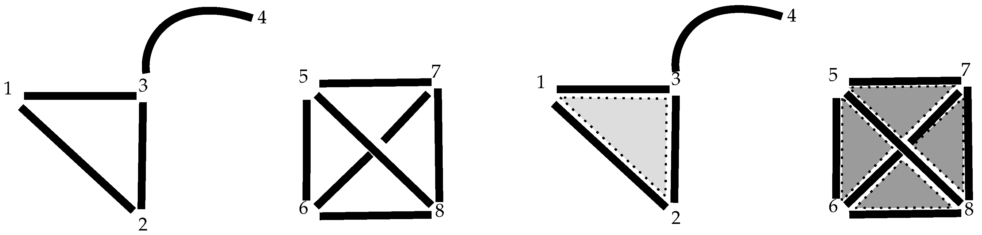
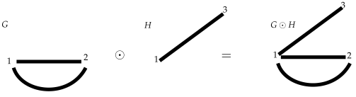
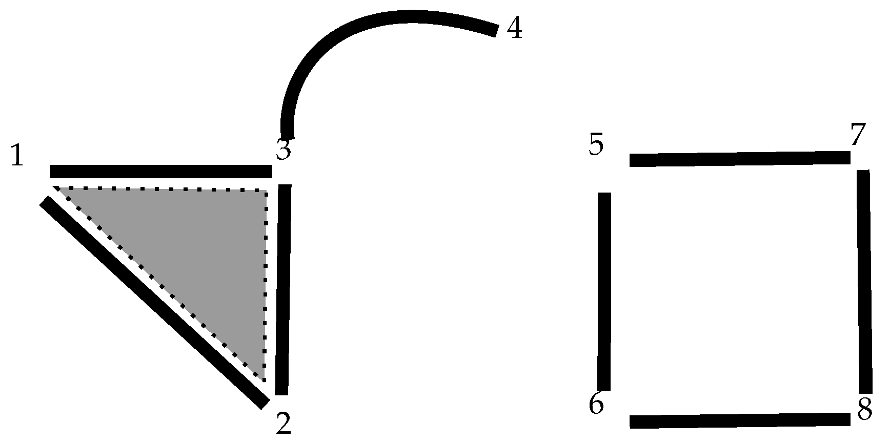
Example 6. The following picture, Figure 4
shows at the left hand side a 4-clique with set of vertices , a 3-clique with vertices and a 2-clique with vertices . Then, it gives rise (on the right) to a complex with a 3-cell, a 2-cell and a 1-cell, respectively. That is, whenever a complete graph is found in one of the connected components of a graph, it converts into a new cell of one less dimension than the clique. In this case we say that a (sub)graphhas been closed or that a cell has been created.
In our notation for the remainder of this paper, we will fill the cells as in the previous example. Observe that we can have a picture such as the following, where the square on the right has not been closed (Figure 5): 4.2. Multicomplexes out of Multigraphs
Since our goal is to give the structure of a simplicial complex to a set of multigraphs (rather than simple graphs), every definition has to be adapted to this setting.
Let
be a simplicial complex with a set of vertices
V and
a
multiplicity function. Now, consider as in [
7] the sets
together with the
gluing functions . Observe that
Here, will allow us to identify every copy of a given cell that belongs to a certain boundary of a higher-level cell. Now, we are ready to introduce the concept of a multicomplex.
Definition 10. Considering the definitions above, a 3-tuple for which every and with the same dimension such that satisfiesis a multicomplex. The elements of are the multicells of . Remark 1. To clarify the above definition, should be seen, respectively, as p- and q-dimensional faces in the multicell while , in its turn, is a non-empty collection of finite subsets of the set of vertices V.
By an abuse of notation, we simply denote by a multicomplex.
Definition 11. Cells with the same vertices in a multicomplex are called duplications.
The following definition is an adaptation for multigraphs of an analogous definition in [
6] for simple graphs. We are from this point deliberately confusing graph and multigraph.
Definition 12. Given a multigraph , its clique multicomplex, denoted by , has the following:
From this point, we will be working with the clique multicomplex that can be defined in ; that is, every clique appearing in a multigraph in the chains of is now seen as a multicell. For a certain , we will denote the multicomplex defined this way as , but we omit the x as often as it does not add any useful information.
4.3. Merging Complexes
Once we have the structure of multicomplexes from multigraphs, we want to define the operation ⊙ for merging simplices rather than graphs. By abusing the notation, we define a binary operation ⊙ for multicomplexes treated as graphs, where we omit the symbols ⊗ in the pictures shown. The reason for suppressing the tensors in the examples is that, once the simplicial complex is constructed out of an element of , the simplices appear just one next to the other. In other words, when we generate simplicial complexes the initial ordering of the multilayer network is forgotten.
From the content above, we notice that closing a multigraph now has a different behavior: it can happen by means of the operation ⊙, as seen in the following.
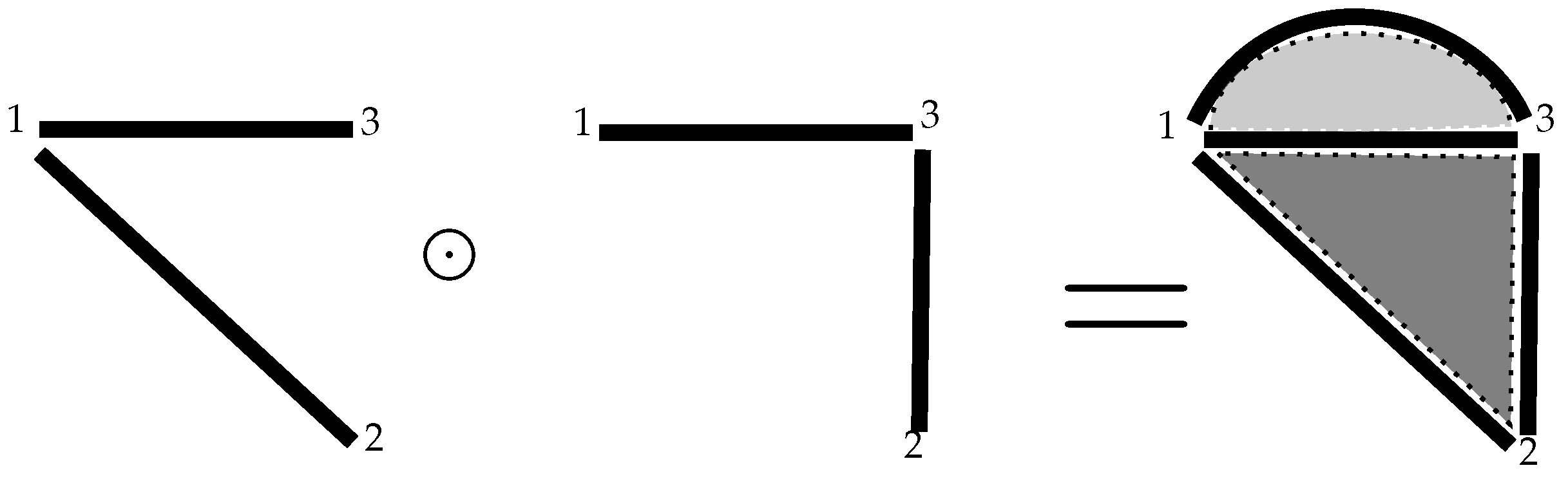
Example 7. In the picture, two 2-simplices have been created (appearing in it with a different tone of grey), Figure 6
whose sets of vertices are both the same: . Of course, we now need to specify each of the 2-cells created in this way, since the boundaries for both are the same, that is, the 1-cells and . It is precisely the function ϕ that allows us to identify them: we now have and with boundariesandrespectively. 4.4. Multiboundaries of a Multicomplex
At this point, we note that not every interaction through ⊙ gives rise to a new cell since it does not always close a graph. On the other hand, a single action of ⊙ could close more than one cell at a time, as happens in the following example.
Example 8. In the following picture, four 2-cells and one 3-cell have been created. Figure 7 Now, for the previous example the following 2-cells have been created, which we detail thanks to
:
as well as the 3-cell
.
It is clear from the picture that we cannot talk about boundaries but rather about multiboundaries.
Definition 13. We define the multiboundary of a multicell aswhich is set is set to be empty in case the dimension of is −1. 4.5. Colouring Multicomplexes
The important characterization for us is of course that of edge-coloured multigraphs, to connect with the example introduced in
Section 2. Therefore, we will continue using the notation introduced in [
7] but considering two key modifications:
Definition 14. Given a finite dimensional complex and a set of colours C, we define a colouring of its 1-cells as a function , where is the set of 1-cells in . We colour a finite-dimensional multicomplex by colouring the underlying complex .
With the notation of the previous definition, one can extend the colouring to all the multicells of
by means of the multisets
for
(where
is the set of j-cells in
) by an abuse of notation. Therefore, a j-cell into
is coloured using as many (possibly repeated) colours as 1-cells it contains.
Example 9. The following graph (Figure 8)
for whichis coloured through the following assignations:where the superindices indicate multiplicity in the multisets built from assignations such as Since the process of merging graphs through ⊙ has to avoid duplicating repeated vertices, there is an ordering for them that has to be preserved along the merging process of graphs. That is, we will enumerate the vertices in such a way that every one appears just once.
Since vertices are seen as , successive are then numbered from them. However, the colours of the 1-cells in the multicells could be repeated, and then we need not just a numbering but also a colour to specify them.
Definition 15 ([
7]).
We denote by the permutation group of the set X and . Let be a d-dimensional coloured multicomplex. We say that is an ordering
if for the assignationis a group homomorphism such that for every there exists such that , where is the action of the permutation on the σ. Now, we need to avoid ambiguities such as the following.
Example 10. In the graph (Figure 9)
we have to distinguish between the 2-cells such that and such that , and for which This is the reason we must consider an orientation of the in a multicomplex. Therefore, from now on the function is thought to be defined on an ordered and therefore the sets of colours generated by it will be also ordered without any further reference. For instance, in the previous example, and .
4.6. The Monoidal Category of Multigraphs
From an algebraic perspective, considering the operation ⊙ for simplices rather than graphs entails the definition of a tensor product for the category of multicomplexes. We have in fact something stronger: it gives to this category the structure of a strict symmetric monoidal category.
The category of coloured multicomplexes was defined in [
7]; we adapt it in a suitable manner for our context and with the notation here introduced.
Definition 16. Let a category with the following characteristics:
Its objects are tuples for , a colouring and p a permutation;
Its morphisms between and are simplicial multimaps ϕ preserving the structure. That is, the following hold:
- -
;
- -
;
- -
.
is the category of multicomplexes to which ⊙ gives a well-known structure.
Definition 17. A strict symmetric monoidal category is a category equipped with an object and a bifunctor such that for objects and morphisms , the following hold:
- -
;
- -
;
- -
;
- -
;
- -
;
- -
.
Lemma 3. is a strict symmetric monoidal category.
Proof. By Definition 2, we have associativity and commutativity. The empty complex ∅ plays the role of a neutral element. □
Observe that in this section we considered multicomplexes consisting of a unique connected component, that is, not coming from chains of graphs but rather from a single multigraph.
5. Filtrations
It is known (see [
14]) that a filtration of a simplicial complex
is just a nested (and totally ordered) set of simplicial complexes
contained in
, that is, a sequence
There is a number of ways of ordering the different
(see [
6] for a nice listing). Filtrations are considered in the context of simplicial complexes as a way to describe and organize the construction of a simplicial complex through a discrete process.
We formalize this complexification process by defining a different concept of filtration. For a certain , we consider the complexes generated by the successive interactions of multigraphs through ⊙, starting from . In the following, we will omit the sub- and the superscript of when the initial graph x is understood from the context or the set of colours C is not relevant.
5.1. Interaction Filtration
This paper introduces a sort of filtration without the form of a totally ordered set, as every other filtration defined so far has to the knowledge of the author, but with that of a partial ordered set. As explained below, this ordering for is inherited by the posetal behavior of .
Let us describe a sort of filtration for
; for this purpose, we see the chains as elements of the complex. Given
and
, let
be the numbers of times ⊙ appears in a chain for the rest of the section.
We will consider for simplicity that every graph in x has a single connected component. Once the simplicial complex is constructed out of an element into , there is no reason to consider ⊗ as a non-commutative operation any more.
For
, the subset
will be called the
level j of the simplicial complex .
Definition 18. The interaction filtration of is the Hasse diagram of the ordering generated out of every application of ⊙ to the initial chain x.
Example 11. For the chain , its interaction filtration is![Ijt 02 00007 i004]() where
where Observe that for a given
k, the bottom of a poset filtration is a chain in the form
and not the empty set; this is one of the reasons why this sequence of complexes does not fit into the formal definition of filtration. On the other hand, the top chain
plays the role of the whole multicomplex (where every interaction has taken place).
Lemma 4. For every , the following fold:
5.2. Results of the Interaction Filtration
A substantial difference with other filtrations, such as those referred to in [
6], is that in ours no more edges appear in every step of the complexification of the filtration. Moreover, to count the steps in the filtration as in [
6], we need something more than simply a chain of pictures (as in the totally ordered models). We will see this from the examples above, where the following lemma is satisfied by any of them:
Lemma 5. Given a simplicial complex with , its interaction filtration is p-folded, where p equals to To construct a full interaction filtration out of k graphs, we count the steps, as performed in the following example. Note that we are considering for simplicity the same colour for all the edges, while they will be coloured in next sections. Take .
Example 12. For , we have ; then, for , if has the form (Figure 10)
Figure 10.
Example 12 (1).
Figure 10.
Example 12 (1).
then for and , and have, respectively, the forms (Figure 11)
Figure 11.
Example 12 (2).
Figure 11.
Example 12 (2).
and finally, for , Figure 12 5.3. Holes in a Multicomplex
As pointed out in the introduction, the main target of this paper is to investigate which of the topological features are preserved through the process of merging graphs in .
We are, in particular, interested in calculating the numbers of holes appearing and remaining along the configurations of an interaction filtration. This is precisely the reason why one should care about filtrations: they provide a way to measure the lifespan of a hole of any dimension in a simplicial complex. This is the field of study of persistent homology, as will be seen in the following section.
To introduce the concept of a hole in a simplicial complex, one needs to define first that of a chain group, cycle and boundary of a simplicial complex (see [
14], for instance). This will be performed in the next section, where it will be seen that, given a simplicial complex
, the
are its connected components, the
are the cavities in
surrounded by edges, the
are voids enclosed by triangles, the
are surrounded by tetrahedrons, etc.
Note that, however, we exclude the cliques of any dimension: a hole is not a clique. That is, a , or a hole of dimension d, in a simplicial complex is a void that is not a clique enclosed by a number of d-simplices.
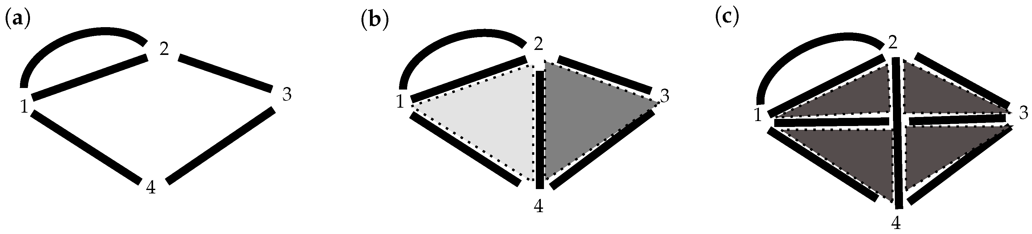
Example 13. Considering the following complexes, Figure 13
we conclude that (a) has one 0-hole and two 1-holes, (b) has one 0-hole, one 1-hole and two 1-cliques, while (c) has one 0-hole, one 1-hole and one 3-clique. Observe that in our notation, cliques are filled with a tone of grey while holes remain blank. Recall also that every time a clique is closed, it is not a hole any more. In the context of a filtration, as increases, the number and complexity of the holes also increase.
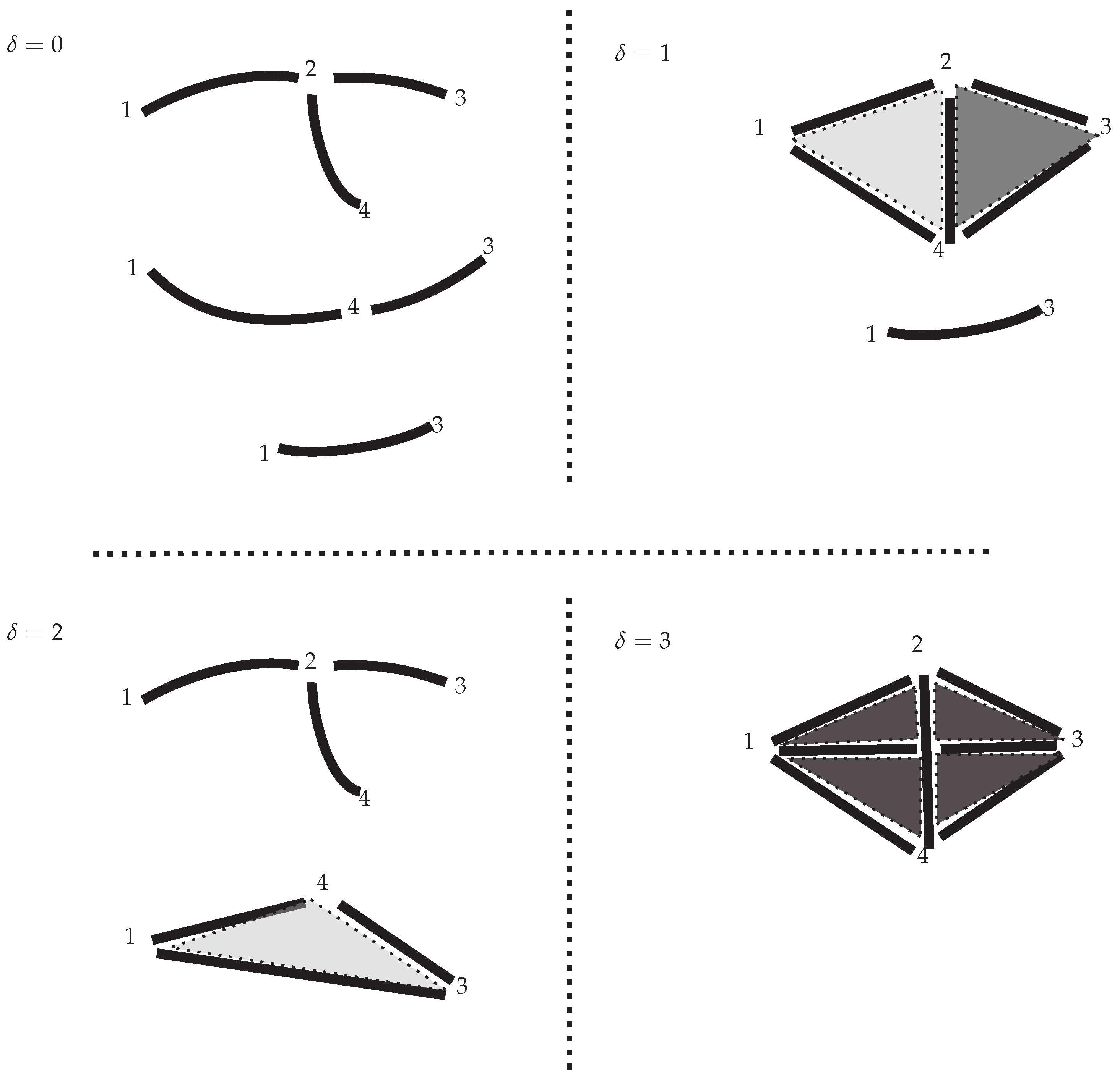
Example 14. For the filtration (Figure 14)
we can identify three 0-holes for , two 0-holes and two 1-cliques for , two 0-holes and one 1-clique for and one 0-hole and one 3-clique for . Notice that this corresponds to a poset withandnaming the graphs involved starting from above. 6. Persistent Homology
Persistent homology serves to quantify some topological features along different configurations of the data; it appears as a way to calculate homology during a (discrete) scale of time. Our aim is to calculate it for our example in [
1], where every application of ⊙ is seen as a step in a certain scale of time. Therefore, it is particularly well suited for our purpose of observing the evolution of the structure introduced.
The idea behind using persistent homology in our concrete neuroscientist context relates to previous work (see [
4]). In that paper, it is shown that some network dynamics can be classified by using topological features such as those computed by persistent homology. The discrete merging dynamic of this paper, in particular, together with the idea of interaction filtration is an example of topological persistency.
Definition 19. The n-chain group of a simplicial complex , denoted by , is the vector space generated by the n-simplices of with coefficients in a field .
That is, the elements of are sums of simplices in . For persistent homology, it is common to use .
Definition 20. The boundary operators of are the linear mapssuch thatwhere we denote by the (n+1)-simplice in composed by these vertices. For this (n+1)-simplice, every tuple is an n-face. 6.1. Betti Numbers
The number of n-holes in the configuration of a filtration is called its
nth Betti number. This is formalized as follows (and see [
14] for an extensive explanation).
Definition 21. The n-dimensional Betti number, denoted by , is the dimension of the quotient Example 15. For the complexes in Example 13, we have , in a), , in b) and , in c).
For the complexes in Example 14, we have when , when , when and when .
From Example 14, we see that, when the number of δ increases, the Betti number of a given dimension decreases; this is coherent with the algorithm provided in [3]. Something more is happening, however, as be seen in the following. 6.2. The Incremental Method
Observe that Lemma 4 says that every chain in a certain
has the same
. It is a natural question to ask how to calculate the first three-dimensional Betti numbers of every chain into the same
; this can be performed by modifying the incremental algorithm designed in [
3].
The results given in [
3] are different from ours since two crucial aspects of the filtration considered are also different. On one hand, for us simplices appear in some steps of the filtration only when they correspond to a clique in the underlying graph. Secondly, we are working with multigraphs here rather than graphs. These two facts make the formula to calculate the Betti numbers more complicated, as will be seen. It appears, however, as a sort of generalization of the one given in [
3].
To obtain the general formula, that working for multicomplexes, we first need some preliminary results. The first lemma corresponds to the incremental method introduced in [
3] for simple complexes (that is, those defined out of simple graphs) and built using a usual filtration. It reconstructs the main result of [
3], which was presented in the form of an algorithm. We refer to
Section 3 of that paper for the exact statement and
Section 3.1 in particular for a detailed explanation of its correctness.
Lemma 6. Let and be simplicial complexes such that is obtained by adding the d-simplex σ to in a filtration process. Then, the following hold:
If σ belongs to a d-cycle in , If σ does not belong to a d-cycle in ,
Let us finish these preliminary results by observing that duplications generate holes. This can be checked in the Examples 13 and 12 above.
Lemma 7. Let and be multicomplexes such that . Each d-dimensional duplication involved in a d-cycle of generates a (d + 1)-hole in .
Now, we are in position of introducing analogous formulae to those of [
3] for multi-complexes built using interaction filtration. The formulae in the following result appear as a sort of
Inclusion–Exclusion Principle for multicomplexes.
Proposition 10. Let be a multigraph and its associated multicomplex. Considering its interaction filtration, the Betti numbers of the configuration are given by the following formulae:where each n is the number of simplices added that close a d-cycle, p is the number of simplices added that do not close a d-cycle, cl is the number of cliques created in each case and dup is the number of duplications for . Proof. The idea is to follow the algorithm designed in [
3] by adapting it to the particularities of merging multigraphs. That is, when adding a new simplice
in an interaction filtration through ⊙ we must distinguish among three possibilities:
closes a
d-cycle in the new configuration,
does not close a
d-cycle in the new configuration and
duplicates an existing simplice in the previous configuration.
It is crucial to observe that interaction filtration is a usual filtration (like that of [
3], for instance) for which we add several simplices in a single step. This allows us to apply the formulae in Lemma 6 to our context. We should be careful, however, with the fact that, from Definition 11, we are closing every clique: since we are counting holes, we have to remove every clique appearing after a new inclusion of a simplice. This points to the Inclusion–Exclusion nature of our formulae.
Therefore, in the first case, and adding one by one the new simplices that close a
d-cycle, we must sum the number of them with the Betti number of the previous configuration. Now, it is time to substract the cycles that convert into cliques, since we are counting
d-holes. (In the expressions
of the formulae there is a flavour to the Morgan Laws in a Logic system). This is a substantial difference with the calculations made in [
3], where cliques are not immediately simplices as in our case and where only one simplice is added in every configuration of the filtration. This case includes parallel simplices, that is, simplices with the same vertices in the underlying multigraph.
For the simplices that do not close a d-cycle, just carry out the same process: step by step add those simplices and calculate accordingly. Observe that the term appears as a consequence of Lemma 7. □
Example 16. (A) For the composition![Ijt 02 00007 i005]() we calculate the following:
we calculate the following: For , we have and and the assignationsas well asand then For , we have and and the assignationsas well asand since we obtain .
(B) For the composition![Ijt 02 00007 i006]() we calculate the following:
we calculate the following: For , we have and and the assignationsas well as, and then For , we have and and the assignationsas well asand since we obtain .
(C) For the composition (where we have not filled the tetrahedron)![Ijt 02 00007 i007]() we calculate the following:
we calculate the following: For , we have and and the assignationsas well asand then For , we have and and the assignationsas well asand since we obtain .
7. Conclusions
A multicomplex structure has been constructed out of an ordered lattice of multigraphs to identify and compute the features of persistent homology. This is performed to observe how much the structure evolves over time, specially the interaction among graphs and the ordering defined. The evolution is characterized by the interaction filtrations, which are defined in this paper. Moreover, for the multicomplex we have introduced an equation that allows us to calculate Betti numbers, that is, the numbers of holes of any dimension.
This should be useful to interpret further extensions on the work about embodiment published so far in the context of Neuroscience. Therefore, this paper should be seen as a very concrete application of persistent homology to that field.


 while
while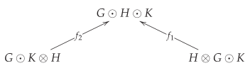 as well as
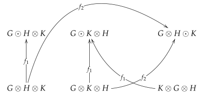

 where
where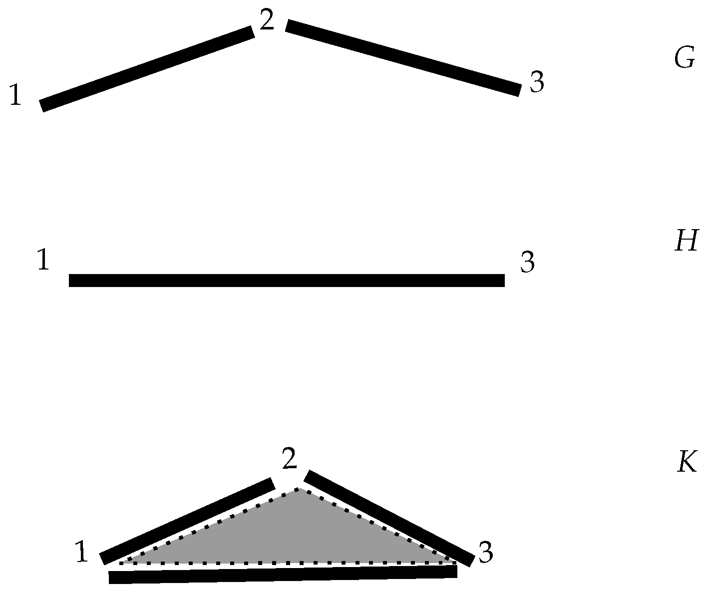
 we calculate the following:
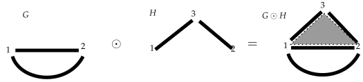 we calculate the following:
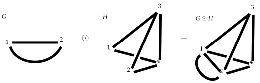 we calculate the following:
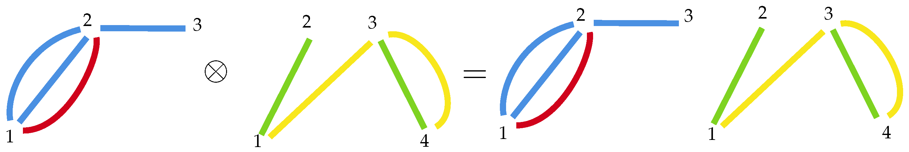


