Macroeconomic and Demographic Determinants of London Housing Prices: A Pre- and Post-Brexit Analysis

Abstract

This study examines the demographic and macroeconomic factors influencing housing prices in London from Q3 2014 to Q4 2022, focusing on the pre- and post-Brexit referendum periods. Using multiple regression analysis, the research evaluates the impact of interest rates, inflation, construction costs, population changes, and net migration on the housing price index (HPI) across various market segments. The findings suggest that interest rate base rates, consumer price inflation, and construction output price indices were significant predictors of housing price fluctuations. Notably, cash purchases exhibited the strongest explanatory power due to a reduced sensitivity to market changes. Additionally, London’s population was a key determinant, particularly affecting first-time buyers and mortgage-backed purchases. These results contribute to a deeper understanding of the London housing market and offer insights into policy measures addressing housing affordability and investment dynamics.

1. Introduction

Housing prices are primarily driven by supply and demand dynamics [1]. Macroeconomic factors such as GDP, inflation, interest rates, and employment play a crucial role in housing price fluctuations [2,3]. Additionally, demographic factors like population growth, migration trends, and construction activity contribute significantly to price determination [4].

The London housing market is one of the most dynamic and expensive real estate markets globally, driven by strong domestic and international demand. Over the years, London has been a magnet for investors due to its economic stability, legal transparency, and cultural significance. The interplay of macroeconomic and demographic factors has shaped its real estate sector, making it a subject of extensive research. Despite ongoing studies, a significant research gap remains in assessing how external shocks—such as the Brexit referendum—have influenced housing prices.

Brexit introduced considerable uncertainty into the UK economy, affecting investment, employment, and consumer confidence. Given that real estate is a long-term investment, changes in government policies, taxation, and regulations related to Brexit have had ripple effects across the housing market. Following the referendum in June 2016 and the official EU exit in January 2020, many speculated that London’s housing prices would decline due to reduced foreign investment and migration restrictions. However, empirical data suggests that while some sectors experienced price declines, others remained resilient due to strong investor confidence and a limited housing supply.

Historically, macroeconomic factors such as GDP growth, interest rates, and inflation have significantly influenced housing prices. The UK government’s monetary policies, including adjustments to the base interest rate, directly impact mortgage affordability and demand. Moreover, supply-side constraints such as rising construction costs and housing shortages have played a crucial role in shaping price trends. Post-Brexit migration-related construction labour shortages reduced the housing supply due to heightening material costs and delayed the housing supply, strengthening housing affordability for new entrants and younger buyers [5]. On the demographic side, London’s population dynamics, including net migration and employment levels, have influenced housing affordability and demand. Global cities like London rely heavily on demographic changes in housing dynamics where, due to the inelastic nature of the housing supply, a modest population growth experiences high demand while population stagnation eliminates supply absorption. Hence increasing and decreasing housing prices accordingly, especially in crisis times such as Brexit [6]. Age composition is another factor affecting the demographic dynamics which increase housing prices [1], with the rise of working residents reinforcing the urban housing demand in London due to job accessibility (see Table A2).

This study aims to provide a quantitative assessment of the key factors affecting London’s housing prices before and after the Brexit referendum. By employing multiple regression analysis as a key tool across different housing market segments, the research seeks to answer the following key questions:

• How did interest rates, inflation, and construction costs impact London’s housing prices?
• What role did demographic factors, such as population growth and migration patterns, play in shaping market trends?
• Were there distinct variations between cash purchases and mortgage-backed purchases in response to economic changes?

By addressing these questions, this study contributes to the broader literature on real estate economics and provides policymakers with insights into potential interventions to stabilise the housing market. The following sections discuss the materials and methods used in the analysis, followed by empirical findings and policy implications.

2. Data Collection and Sources

This study is based on a comprehensive dataset spanning from Q3 2014 to Q4 2022, capturing economic, demographic, and housing market-specific indicators that have influenced London’s real estate prices before and after Brexit. The dataset includes macroeconomic and demographic variables obtained from the following:

• The Greater London Authority: Population and labour market statistics specific to London.
• The UK Office for National Statistics (ONS): GDP growth, inflation (Consumer Price Index including Owner Occupied Housing Costs in All items—CPIOOHC), interest rates, net migration, and employment and unemployment figures.
• The Bank of England: Historical interest rate base rates.
• The National House-Building Council: Data on new builds, housing starts and completions.
• The UK Land Registry: Housing price indices (HPI) for different market segments.

The dataset was converted into a quarterly format to maintain consistency across indicators and account for macroeconomic trends. Given the importance of Brexit-related events, particular attention was paid to the period from Q2 2016 (referendum quarter) to Q4 2022 to assess its long-term impacts on housing prices.

2.1. Dependent Variable

The London House Price Index (HPI) serves as the dependent variable, measured across six different housing market segments:

• HPI—Cash Purchases
• HPI—Mortgage Purchases
• HPI—New Builds
• HPI—All Property Types
• HPI—First-Time Buyers
• HPI—Former Owner-Occupiers

These categories allow for a granular analysis of how different buyer groups were impacted by macroeconomic and demographic factors, demonstrated monthly in Table A5 and Figure A1, and quarterly in Table A6 and Figure A2.

2.2. Independent Variables

The following independent variables were included in order to capture a comprehensive view of London’s housing market:

• Macroeconomic Indicators:
  • UK GDP Growth (%)—quarterly growth rate to capture economic activity.
  • Consumer Price Index including Owner-Occupied Housing Costs (CPIOOHC, %)—inflation measure.
  • UK Interest Rate Base Rate (%)—indicator of monetary policy and borrowing costs.
  • Construction Output Price Indices (COPI, %)—proxy for housing supply costs.
  • Trade Balance (£ millions)—the UK’s total exports minus total imports.
• Demographic Indicators:
  • London Population (millions)—capturing housing demand fluctuations.
  • Net Migration (thousands)—proxy for international demand for housing.
  • London Median Pay (£)—reflecting wage growth and affordability.
  • Total Employment in London (thousands)—indicating workforce growth.
  • Unemployment in London (thousands)—assessing job market fluctuations.
• Housing Supply Variables:
  • New Build Housing Starts (thousands)—indicator of supply expansion.
  • Housing Completions (thousands)—capturing realised supply additions.

2.3. Rationale for Excluded Variables

While stock prices could provide insights into wealth effects and overall market sentiment, they were omitted from this study. The significance of stock prices in real estate trends is also highlighted [7]; however, their inclusion could introduce excessive volatility unrelated to Brexit-specific housing market shifts. Stock prices reflect broad global financial movements, which may obscure the localised effects of macroeconomic and demographic variables on London housing prices.

The independent variables selected in this study were chosen for their direct relevance to London and the broader UK real estate market. These selections align with prior research on housing price determinants [2,3,5,6,7,8,9,10,11,12,13,14,15,16,17,18,19].

2.4. Biases of Data

While efforts were made to ensure the reliability and accuracy of the dataset, potential biases may still exist due to data collection methodologies, limitations in publicly available information, and economic uncertainties surrounding Brexit. The key biases identified in this study are outlined below:

• Data Collection Bias:

The study relies on official statistics from sources such as the Office for National Statistics (ONS), the Greater London Authority, and the Bank of England. While these institutions adhere to strict quality controls, government-reported data may still be influenced by political interpretations or methodological constraints. For instance, GDP revisions and inflation recalibrations could lead to discrepancies over time.

• Timeframe Bias:

The dataset covers the period from Q3 2014 to Q4 2022. While this timeframe captures both pre- and post-Brexit housing market trends, it may not fully account for long-term structural changes in London’s housing sector. Additionally, external shocks such as the COVID-19 pandemic and the Suez Canal blockage may have introduced confounding variables that are difficult to isolate within the dataset.

• Selection Bias in Housing Price Index (HPI):

The study focuses on the UK House Price Index (HPI) and its subcategories (cash purchases, mortgage-backed purchases, new builds, etc.), which are based on completed transactions. This approach may underrepresent off-market deals, corporate acquisitions, and foreign investment transactions that do not follow conventional purchasing routes.

• Exclusion of Microeconomic Factors:

Certain property-specific characteristics (e.g., square footage, age of property, proximity to amenities) were not included in this study due to data constraints. While the macroeconomic and demographic variables selected provide a broad understanding of price trends, omitting micro-level property data may reduce the precision of certain findings.

• Migration Data Limitations:

Net migration figures are based on estimates and may not fully capture the real movement of individuals in and out of London. Factors such as short-term employment contracts, student migration, and Brexit-related policy changes may have created unrecorded fluctuations in actual residency patterns.

• Monetary Policy Impacts:

The Bank of England’s interest rate adjustments were a significant independent variable in the study. However, interest rate impacts may differ based on mortgage lending conditions, borrower risk profiles, and lending regulations, which were not explicitly accounted for in this analysis.

• External Economic Influences:

The study’s focus on Brexit as a primary economic event may inadvertently downplay other global economic forces, such as fluctuations in international trade, foreign direct investment, and global financial market trends, which could have concurrently influenced London’s housing market.

• Mitigation Strategies:

Recognising these potential biases, several strategies were employed to enhance the robustness of the findings and ensure a balanced analysis of London’s housing market trends. These measures aimed to minimise data distortions and improve the study’s reliability:

• The study incorporated multiple sources to cross-validate key macroeconomic indicators.
• Adjustments were made using base quarter recalibrations to account for structural shifts in the housing market pre- and post-Brexit.
• Limitations were acknowledged, and future research directions were proposed to incorporate additional microeconomic factors and extend the timeframe of analysis.

By recognising and addressing these biases, this study aims to provide a balanced and data-driven assessment of the factors influencing London’s housing market trends before and after Brexit.

3. Multiple Regression Analysis

The decision to adopt Multiple Regression Analysis was due to its major statistical technique, and the fact that it is the most relevant based on previous studies, [3,20], which examined the housing prices estimation on a cause-and-effect analysis on independent variables. Relevant studies used regression analysis on macroeconomic factors in estimating London house prices [3], while others employed Multiple Regression Analysis on pooled cross-section timeseries data [20], where house prices, acting as the dependent variable, were log transformed and explained by the variability of independent variables. Collecting a cross-sectional dataset contributed to the selection of the methodology used to estimate housing prices during this study period. Alternatively, VAR could have been adopted as it requires variables as interdependent and endogenous and it incorporates multiple time series simultaneously of the same frequency, leading to more dynamic variable interactions and a more comprehensive analysis [21]. This may be considered a more suitable methodology for this study, as it was used in previous studies to identify the interactions between variables such as interest rates, inflation, GDP, unemployment, and housing prices [22,23]. However, this methodology was eliminated from this study due to the time dependency of the data and their variation of data frequency (monthly and quarterly) since, when aggregating monthly or interpolating quarterly data, a loss of information or inaccuracies can occur [24] resulting in less reliability in model estimation and interpretation [25]. MRA was chosen because it focuses on the explanation of a single variable outcome through several estimations omitting any time interaction [23]. Vector Autoregression (VAR) was eliminated from this study due to the limited data collected, as it typically requires 100 to 500 observations per variable for a more robust variable estimation and the minimising of standard errors [26].

The equation of the Multiple Linear Regression (MLR) model is formulated as follows:

• y = β0 + β1x1 + β2x2 +…+ βpxp + ϵ
• Y = dependent variable
• β0 = represents the intercept
• β1, β2, ….βp= represent the coefficients of the independent variables x1, x2…xp
• x1, x2…xp = represent the independent variables in the model
• ε = represents the error term
• β0 and β1 = represent the regression coefficients in the model [27]

3.1. Correlation Coefficient

Additionally, Correlation Coefficient, R-Squared, and Adjusted R-Squared were employed to assess the linear relationship and the intensity within this relationship between two quantitative variables. R-squared (R2) represents the percentage of the variation in the dependent variable which is explained by the independent variables in the sample, whereas the adjusted R-squared (R2) represents a corrected R-squared, providing a more accurate goodness-of-fit in the regression model with different numbers of predictor variables [28,29].

The correlation strength is recognised by the range of −1 to 0, and 0 to +1 between two variables, where a positive sign of correlation coefficient indicates that a positive correlation exists, whereas carrying/holding a negative sign of correlation coefficients indicates that a negative correlation exists between data [30,31]. In addition to this, interpretational indications of the Strength of Correlation as to the size of “r” are demonstrated below in Table 1.

Table 1. R-square interpretation.

Size of “r”	Interpretation
0.90 to 1.00	Very high correlation
0.70 to 1.89	High correlation
0.50 to 0.69	Moderate correlation
0.30 to 0.49	Low correlation
0.00 to 0.29	Little if any correlation

Refs. [30,31] This study assumes a linear association between a log-transformed dependent variable and multiple independent variables, some of which holding positive signs were log transformed.

The equation of the logarithm transformation is as follows:

Log(y) = β0 + β1x1 + β2x2 + … + βpxp + ϵ

(1)

log(y) is the natural logarithm of the dependent variable y [32].

3.2. Descriptive Statistics

Descriptive statistics were employed to identify each independent variable’s mean, the standard deviation and the coefficient of variation as adopted in studies of [32,33]—descriptive statistics in Table A2—which identified that the mean values of London Median Pay were substantially lower compared to the London House Price Index and House Price Index in all property types, evidently confirming the reliance on financing on home purchases, while base interest rates enhance the sensitivity on London House Prices in relation to London median pay.

During this study period, net migration constituted 3% of London’s population, which is a considerably low population proportion and likely to be attributed to the unaffordability of housing and low median pay in London as previously suggested by the findings of [12,19,34], while high migration outflows were substantial further to the Brexit referendum based on the studies of [35].

Additionally, the negative mean value of the Trade Balance (7136.62) GBP depicts higher import tariffs and higher production and transportation costs, which leads to increasing construction costs, subsequently increasing house prices.

Furthermore, London population (aged 16–64) mean values show that 51% are in employment, whereas 6% are unemployed (see Table A2), demonstrating the regional high employment rate.

Standard deviation was used to examine the robustness of the data, interpreted through the coefficient of variation (see Table A2 and Table A3), analysing the standard deviation over the mean. It is calculated using the following formula [32,33]:

CV = Mean/Standard Deviation

Applying the coefficient of variation as shown in Table A3 identified this study’s data with the highest variability around the mean. Among those were the GDP Quarter on Quarter Growth (1034%), the Trade Balance (−166%), the ‘consumer price index occupiers’ housing costs in all items’ (97%), and the Interest Rate Base Rate (94%) which vary substantially over time causing inaccuracy on the estimations.

3.3. Multicollinearity

Table A4 demonstrates the correlation matrix using Excel which examines the multicollinearity between two or more independent variables on Q3 2014 to Q4 2022. Correlation coefficients holding values higher than 0.70 were eliminated from this study, thereby providing more accurate data results, hence accurately providing a coefficient estimation in the regression model [32,33].

3.4. Base Quarter Adjustment

The Brexit referendum effect was reflected setting Quarter 2 (Q2) 2016 as the Base Quarter for London housing prices, where prices were adjusted by adding 1% to 5% concerning the Q3 2014 to Q4 2015 and subtracting 2–15% on Q1 2017 to Q4 2022.

The rationale behind the percentages used from a structural break theory perspective was to isolate structural economic shocks, such as Brexit, in order to normally adjust in a non-crisis reference period. From an expectations-driven theory perspective and associated behavioural response, the ad hoc approach was adopted: 1% percent for each quarter before the Brexit referendum, subtracting 1% for each quarter post-Brexit referendum, ensuring a more stable stage of comparison. This upward adjustment reflected speculative optimism and anticipation, and the downward adjustment the increased uncertainty.

3.5. Correlation Matrix

Further conducting a correlation matrix, highly correlated data were eliminated from the study, such as the London Average price index in All property types, London Population, Population per hectare, Population per square kilometre, Number of London Residents in employment All aged 16 to 64, London Employment rate (%), London Unemployment rate (%), and the long-term international migration into and out of the United Kingdom by nationality including British, EU, Non-EU. Additionally, various highly correlated independent variables were kept in the model due to being considered totally independent variables which are further explained, while some others were removed from the data set to fit the model more accurately. See Table A4.

3.6. Log Transformation

Log transformation with base 1000 was adopted in all of the seven models of Dependent Variables (House Price Indices) to meet the above-mentioned assumptions of the method, normality, and linearity. However, some of the independent variables were not log transformed due to their inclusion of negative values, such as Gross Domestic Growth Quarter on Quarter growth, Interest Rate Base rate, Consumer Price Index owners occupied housing costs in all items, and All starts of dwellings, all completions of dwellings and trade.

Certain log bases were chosen for improved numerical stability—enhanced model coefficient interpretability that are measured on vastly different scales. This effectively allowed the rescaling of variables to have manageable numeric ranges from 0–1. Additionally, this aids data visualization and plotting, which allows for comparability.

3.7. Goodness of Fit

The goodness of fit of the models were identifying and interpreted through the use of R-square and Adjusted R-square, whereas the f-test was employed to identify the statistical significance of each model and p-value the statistical significance of the coefficients.

3.8. Model Selection

Akaike Information Criterion (AIC) was employed to assess the goodness of fit with model complexity when comparing models [27], while the models with the lowest AIC values were chosen through eliminating competing regression models from overfitting (see Table 2).

Table 2. Model data results.

		Model 1: HPI Cash Purchases	Model 2: HPI Mortgage Purchases	Model 3: HPI New Build	Model 4: HPI in All Property Types	Model 5: HPI First-Time Buyers	Model 6: HPI Former Owner-Occupiers	Model 7: HPI Mortgage Purchases
Regression Statistics	Multiple R	0.967702515	0.95506282	0.958167847	0.958145046	0.959424326	0.955500929	0.28918806
	R Square	0.936448157	0.91214499	0.918085624	0.91804193	0.920495038	0.912982025	0.083629734
	Adjusted R Square	0.900132819	0.861942127	0.871277409	0.871208747	0.875063631	0.863257467	0.024509071
	Standard Error	0.003178484	0.003416828	0.004176872	0.003362874	0.003482584	0.003241064	0.009082475
	Observations	34	34	34	34	34	34	34
ANOVA	RSS (Residual SS)	0.000212158	0.000245169	0.000366372	0.000237487	0.000254696	0.000220594	0.002557232
	n (No. of Observations)	34	34	34	34	34	34	34
	k (No. of parameters)	13	13	13	13	13	13	3
	AIC (Akaike)	−381.4743533	−376.5573927	−362.8995436	−377.6397787	−375.2612138	−380.1486039	−316.8364776
	BIC	−12,924.28532	−12,757.10866	−12,292.7418	−12,793.90979	−12,713.03858	−12,879.20985	−10,761.86116
	F-Statistic	25.78657368	18.16918273	19.61377131	19.60238171	20.26120471	18.36078739	1.414560164
	p-value	7.31 × 10−10	1.9−4 × 10−8	9.6 × 10−9	9.64932 × 10−9	7.09839 × 10−9	1.76538 × 10−8	0.258285681
Coefficients	Intercept
	Coefficient	−2.600954066	−2.566576162	−2.472436333	−2.571138851	−2.619735914	−2.514935524	0.679667238
	Standard Error	0.325386547	0.349786261	0.427593195	0.344262835	0.356517725	0.331792957	0.002659017
	t-Statistic	−7.993428397	−7.33755566	−5.782216278	−7.468534484	−7.348122491	−7.579833958	255.6084148
	p-value	8.34448 × 10−8	3.19883 × 10−7	9.70434 × 10−6	2.43468 × 10−7	3.12889 × 10−7	1.93416 × 10−7	4.27502 × 10−53
Log with base 10,000,000 London population	Coefficient	4.338218502	5.16631317	3.901809254	5.007341692	5.038470513	4.980515121
	Standard Error	1.616135995	1.737324953	2.123777888	1.709891093	1.770758913	1.647955473
	t-Statistic	2.684315253	2.973717243	1.837202127	2.928456504	2.845373515	3.022238891
	p-value	0.013883976	0.007243641	0.080373974	0.00802945	0.009689464	0.006483471
Log with base 1,000,000 Net Migration	Coefficient	0.062681314	0.062367768	0.031374487	0.061869673	0.061475409	0.062959768
	Standard Error	0.028487861	0.030624076	0.037436137	0.030140495	0.031213421	0.029048747
	t-Statistic	2.200281525	2.036560006	0.838080241	2.052709226	1.969518445	2.167383253
	p-value	0.039117417	0.054498953	0.411423444	0.052770593	0.062226963	0.041848397
GDP	Coefficient	0.000108233	0.000116174	6.94176 × 10−5	0.000113608	0.000106428	0.000125175
	Standard Error	0.000216776	0.000233032	0.000284867	0.000229352	0.000237516	0.000221044
	t-Statistic	0.499282725	0.498533623	0.243684023	0.495344172	0.448086374	0.56629078
	p-value	0.622770671	0.623289497	0.809840328	0.625500746	0.658679556	0.577198546
IR base rate	Coefficient	−0.009740763	−0.010344908	−0.01071233	−0.010173949	−0.010501916	−0.009948918	0.001955025
	Standard Error	0.003227997	0.003470054	0.004241938	0.003415259	0.003536834	0.003291552	0.005212322
	t-Statistic	−3.017587741	−2.981195073	−2.525338979	−2.978968587	−2.969298806	−3.02256173	0.375077494
	p-value	0.006552871	0.007121141	0.019669438	0.007157405	0.007316973	0.00647868	0.710156868
CPIOOHC in All items	Coefficient	0.004749632	0.004383166	0.003174663	0.004472918	0.004408887	0.004559121	−0.001808049
	Standard Error	0.001160547	0.001247572	0.001525084	0.001227872	0.001271581	0.001183396	0.001183686
	t-Statistic	4.092581685	3.513355892	2.081631749	3.642820794	3.467247707	3.852573716	−1.527474469
	p-value	0.00052074	0.002066209	0.049797564	0.001521124	0.002303457	0.000923717	0.13678309
Log with base 10,000 of London Median Pay from PAYE	Coefficient	−0.145938843	0.017817145	−1.258856285	−0.01575365	−0.137881457	0.155758213
	Standard Error	0.649863534	0.698594757	0.853991129	0.687563343	0.712038868	0.662658446
	t-Statistic	−0.224568444	0.025504264	−1.474085903	−0.022912289	−0.193643161	0.235050521
	p-value	0.824485663	0.979893554	0.155292266	0.981936558	0.848316085	0.816446365
Log with base 10,000,000 of Total in employment	Coefficient	−0.994933785	−2.123612792	−0.386135756	−1.904294316	−1.825081571	−2.026293278
	Standard Error	1.828451101	1.965560901	2.402782953	1.934522998	2.003387149	1.864450769
	t-Statistic	−0.544140221	−1.08041058	−0.160703552	−0.98437409	−0.910997942	−1.086804389
	p-value	0.592076184	0.292211775	0.873862789	0.336137911	0.372635547	0.289440911
Log with base 1,000,000 of Unemployed (’000s)	Coefficient	−0.011124499	−0.024665574	0.054365975	−0.021285141	−0.017855857	−0.027063273
	Standard Error	0.077591882	0.083410253	0.101964144	0.082093133	0.085015442	0.079119558
	t-Statistic	−0.143371949	−0.295713928	0.533187184	−0.259280411	−0.210030743	−0.342055409
	p-value	0.887363276	0.770352825	0.599502086	0.797943638	0.835668039	0.735708739
COPI	Coefficient	0.008549181	0.010003936	0.008414233	0.009672236	0.009645061	0.00975438
	Standard Error	0.001841924	0.001980044	0.002420488	0.001948778	0.002018149	0.001878189
	t-Statistic	4.641440359	5.052379884	3.476254636	4.963232516	4.779161414	5.193502525
	p-value	0.000140326	5.29697 × 10−5	0.002255103	6.5377 × 10−5	0.000101126	3.80079 × 10−5
Trade Balance	Coefficient	−0.027349689	0.106369466	0.718507614	0.076553141	0.119106688	0.024831248
	Standard Error	0.306902041	0.32991566	0.40330255	0.324706007	0.336264724	0.312944517
	t-Statistic	−0.08911537	0.322414116	1.781559808	0.235761395	0.354205122	0.079347127
	p-value	0.929834657	0.750326849	0.08929009	0.815901894	0.726716984	0.93750779
All Starts	Coefficient	0.029521422	0.023898569	0.020265601	0.024841983	0.025888478	0.023021625
	Standard Error	0.058081652	0.062437012	0.076325587	0.061451078	0.063638582	0.059225199
	t-Statistic	0.508274491	0.382762848	0.265515171	0.404256265	0.406804765	0.388713342
	p-value	0.616558732	0.705742392	0.793201727	0.690111888	0.688267762	0.701401341
All Completions	Coefficient	−0.015633461	−0.033749658	−0.032085397	−0.029597887	−0.025695669	−0.035679074
	Standard Error	0.08125193	0.087344756	0.106773843	0.085965507	0.089025663	0.082851668
	t-Statistic	−0.192407261	−0.386395925	−0.300498657	−0.344299568	−0.288632152	−0.430637971
	p-value	0.849271708	0.703090728	0.766751559	0.734044909	0.775692724	0.671119249

3.9. Regression Analysis Results

For the statistical analysis of the data, multiple linear regression was employed in Excel in all the seven models, emphasising the statistical results on the R-square statistic, significance tests of p-value, and the coefficients. After adopting the method of correlation matrix and eliminating the independent variables that achieved multicollinearity, following an adjustment of both the dependent and independent variable to reflect the base quarter of Q2 2016, we conducted a regression analysis on various types of HPI in London. In terms of outliers, using the Interquartile Range (IQR), the outliers were identified on the three first quarters of 2020 when Brexit occurred that had significant effects on the variables selected. These outliers could not be omitted from the regression analysis due to causing models’ lower goodness of fit, and net migration was not found statistically significant in the models. Further conducting such an analysis, we obtained the best-fitting models with the highest R-square and Adjusted R-square with statistically significant models and coefficients.

In all of the models where the dependent variable was log transformed, the transformations were applied using the natural logarithm, such as ln(1000 × Y) ln(1000 × Y) for the House Price Indices, ln(10,000,000 × London Population) ln(10,000,000 × London Population), ln(1,000,000 × Net Migration) ln(1,000,000 × Net Migration), ln(10,000 × London Median Pay from PAYE) ln(10,000 × London Median Pay from PAYE), ln(10,000,000 × Total in Employment) ln(10,000,000 × Total in Employment), ln(1,000,000 × Unemployed (000s)) ln(1,000,000 × Unemployed (000s)), and similarly for the other independent variables, Gross Domestic Product Quarter on Quarter growth, Interest Rate Base Rate, consumer price index occupiers’ housing costs in all items, Construction Output Price Indices Housing, Trade Balance, All starts, All Completions remained the same values.

3.10. Regression Equation

The regression equation was calculated as follows in all the following models:

Log1000(Y) = b0 + log Logarithm 10,000,000 (b1 X1) + log 1,000,000 (b2 X2) + b3 X3 + b4 X4
+ b5 X5 + log10,000 (b6 X6) + log10,000,000 (b7 X7) + log1,000,000 b8 X8 + b9 X9
+ b10 X10 + b11 X11 + b12 X12 + ε

The unstandardised beta coefficients represented by b1 to b12, representing the slope, correspond to the expected change of the dependent variable deriving from a corresponding one-unit change in an independent variable. In this model, the unstandardised beta represents the percentage change on a dependent variable from one percentage point change in an independent variable. The models adapted log transformation on most of the independent variables and dependent variables where the application was allowed. Therefore, the interpretation of the beta coefficients needs to be transformed in some cases. In cases where both the dependent and independent variables are log transformed, the interpretation will be that a 1% increase in the independent variable corresponds to the percentage increase of the beta coefficient on the dependent variable. In cases where the dependent variable is solely log transformed and the independent variable has not been transformed, the beta coefficient of the independent variable will be the presented value or in percentage form (%).

4. Results and Discussion

In terms of goodness of fit, Model 1 held the highest R-square (r = 0.936) and Adjusted R-square (r = 0.900) among other models, where Model 1 independent variables explained the variation of the dependent variable to a greater extent and held a very low unexplained variation. This suggests that the model independent variables are strongly correlated (see Table 1) in predicting the housing prices in cash purchases, since one third of London are foreign investors [34]. This may be attributed to their reduced sensitivity in market economic alterations, which aids in predicting a more stable and accurate estimation of housing prices, reduced transaction costs compared to mortgage purchases, which improves the consistency and data quality, and lastly to the demographics of those buyers, who are generally high-net worth individuals that contribute consistently on the HPI.

4.1. Model Selection

Consistently with the goodness of fit, the comparison amongst the seven models through Akaike Information Criterion (AIC) found that Model 1 held the lowest value amongst the other models, which demonstrates the best balance of goodness of fit and complexity (see Table 2).

4.2. Statistical Significance

Further conducting regression analysis on the seven models, the statistically significant independent variables were interpreted along with their unstandardised beta coefficients and the linear relationship was confirmed. The data results show that housing prices in London are significantly dependent on the interest rate base rates, with their expected negative signs, along with inflation (consumer price index occupiers’ housing costs in all items) and the construction costs (construction output price indices housing) with their expected positive signs (see Table A1). They are demonstrated in models 1 to 6 (see Table 2) and depict their great impact on the housing prices, which are aligned with previous findings [36].

Additionally, construction output price indices housing was found to be statistically significant and acted as the second greatest contributor with the expected effect (positive sign) in all of the best-fitting models, based on its unstandardised beta coefficients, exhibiting a 0.84% increase in prices with every associated construction output price increase in models 1 and 2 (see Table 2). Hence, construction cost increases do not affect to a great extent new build buyers as mortgage buyers, which recorded an expected increase of 1.07%.

This evidently shows a consistency with previous study findings [36] with a positive correlation between construction costs and the inflation of housing prices. It is also consistent with more recent studies [37] which found that building materials increased due to Brexit, COVID 19, and trade limitations caused by the Suez Canal blockage, thereby demonstrating how the rational and expected effect of inflation and costs on construction affects the rise of housing prices. However, this is in opposition to the finding that the construction costs decline lasted for a short period of time further to Brexit [38]. Construction output price indices housing held the highest contribution in Model 2 (HPI in mortgage purchases) (see Table 2) amongst the other independent variables, demonstrating that construction costs in relation to mortgage purchasers cause the most substantial increase on the dependent variable. This depicts that construction costs may be directly associated with new build properties that require construction, consequently leading us to the fact that most of the mortgage purchasers require a new build rather than an existing property. Therefore, it is vital to conduct further research focusing on specific property types (new builds preferably) and how they interact with mortgage buyers.

Inflation (consumer price index occupiers’ housing costs) holds the lowest unstandardised beta coefficient among the other independent variables that were marked statistically significant in all of the models (interest rates base rate and construction output price indices housing). It was vital to include the interest rates base rate in the model since they were closely associated and interacted with each other, as previous evidence suggests [15]. This is also supported by their multicollinearity effect, as demonstrated by their correlation (r = >0.9) (see Table A4). The results evidently show consistency with the previous bibliography which shows that inflation acts as a great enhancement on the housing market prices in London, with the expected sign (increase) (see Table A1) demonstrated in the results of models 1–6 (see Table 2). This is consistent with previous study findings [2] during the period 1996–2016, when there was a 76% rise in inflation in the UK and mean prices quadrupled, marking the period before the Brexit referendum. This was followed by an increasing rate of inflation and an associated increase in housing prices, which is supported in earlier studies [36]. This was distinctly evident in the local market [39] where recorded consumer price inflation rose in the following two years further to the Brexit referendum.

Net Migration was not found to be statistically significant in any of the best-fitting models, HPI mortgage purchases (model 2), new build (model 3), and first-time buyers (model 5), which was contrary to our expectations (see Table A1). However, this independent variable was found statistically significant in model 1 (HPI cash purchases), model 4 (HPI in all property types), and model 5 (HPI Former Owner-Occupiers) (see Table 2), while holding the second largest contribution amongst other independent variables in those models, as demonstrated in its unstandardised beta coefficient. However, this contradicts earlier studies [3,12] that found that housing prices in Greater London suffered as a result of emigration in a pre-Brexit referendum study, and this was further supported in post-Brexit studies [34,35] that identified low immigration in London and emigration from London, respectively.

However, this can be explained by the fact that net migration is a considered a great contributor to the housing prices of London due to foreign high net worth individuals or cash buyers. This is supported by the fact that it has only affected the HPI of the models that incorporated cash buyers and HPI in all property types as well as former owner-occupiers, who may not require a mortgage due to their purchasing power in purchasing an additional property. This is evidently supported by the studies where the housing prices are mostly influenced by migration and income [11] and the large proportion (one-third) of foreign investors in the London housing market [34]. This highlights the affordability issue that exists in London which is further enhanced through the lack of housing supply in highly dense areas of London and the lack of incentives on affordable housing.

The greatest contributor was London Population amongst all statistically significant independent variables in all of the best-fitting models, cross-referenced by the range of the descriptive statistics over the years (see Table A2), except in model 3, with the dependent variable HPI in new build (see Table 2). In models 1, 2, 4, 5 and 6 it was found to be the most important independent variable for the explanation of the variance of the dependent variables for housing prices, especially in model 2 (HPI in mortgage purchases) and model 5 (HPI in First-time buyers) where its unstandardised beta coefficient held the highest contribution on the dependent variables, with b = 5.166 and b = 5.038, respectively (see Table 2). This shows that the London population is the most influential factor amongst the other selected independent variables in housing prices, which means that as the population increases (by 1%) the demand for housing increases as well, leading to a 5% housing price growth, the impact of which is approximately numerically consistent with previous studies [3,12]. The other models 1, 4, and 5 (HPI in cash purchases, all property types and former owner-occupiers) also held the London population as the greater contributor in the model with a value of unstandardised beta coefficients of b = >4, meaning that housing prices are expected to experience a 4% rise with every 1% increase in the London population (see Table 2). The above results showcase consistency with the earlier critical findings [3], of the strong effect of the population increase, with slightly lower results, with a 5.3% increase in housing prices (NHPI) with every 1%. This shows a consistency with the previous literature and findings. Therefore, the London population and Net migration were only statistically significant in models 1, 2, 4, 5 and 6 and models 1, 4, and 6, respectively, (see Table 2). This is also consistent with the findings of [3], which demonstrated the great influence that the London population had on the NHPI; similarly, consistent findings that found that population is one of the greatest contributors amongst other variables that influence the House Price Index [36].

The interest rate base rate has an expected negative sign due to the negative impact it has on mortgage buyers who have a distinctly greater impact on HPI on mortgage purchases than in model 1 HPI cash purchases (see Table 2). Hence, as expected, the interest rates base rate affects mortgage purchases to a greater extent than it does cash purchases. Model 2 in Table 2 exhibits a distinctively lower increasing rate in the HPI due to the incorporation of mortgage since construction costs and inflation increases, as expected, due to reducing the ability of mortgage purchasers to buy real estate in London, thus excluding them from the market. Similarly, the same impact is found in the interest rate base rate raise for mortgage buyers, and to a higher extent, recording a b = −0.01035 (or −1.35% in HPI mortgage purchases), as opposed to model 1 (dependent variable HPI cash buyers) (see Table 2).

Model 3, (see Table 2), shows that cash buyers may seek for a resale of existing dwellings rather than new builds due to their relatively higher price. These buyers may be potential investors who seek higher returns, therefore the new builds are not as attractive for them. There is a lower contribution and therefore lower increase in the HPI in new builds from the consumer price index occupiers’ housing costs, recording a 0.317% rise with every associated one-unit increase (%) in consumer price index occupiers’ housing costs. This shows that inflation prevents people from buying new builds and encourages the resale of existing dwellings.

Moreover, a further model was conducted, model 4, with the dependent variable (HPI in all property types) in which the results were similar to model 1, with the same statistically significant independent variables as in model 1 (see Table 2). This showed that the HPI is mostly driven up by cash buyers, emphasised by the results of the more generic HPI (HPI in all property types) that had the same effect as the HPI in cash buyers. Most importantly, the net migration variable is more distinct when examining the HPI of cash buyers and in all property types, which shows that people migrating to London are great contributors to housing price increases.

After conducting a regression analysis on dependent variables including the HPI of First-time Buyers (model 5) and Former Owner-Occupiers (model 6) both were log transformed. The results showed that in all the dependent variables (HPI), the interest rates base rate, consumer price index occupiers’ housing costs, and construction output price indices housing were the largest contributors and statistically significant independent variables in all of the models. The London population was also a great contributor on the housing price apart from the HPI in new builds. The net migration was found important and statistically significant in models 1, 4 and 6, which involved cash buyers, former owner-occupiers, and the general HPI in all property types (see Table 2).

The regression residual plots were conducted, and we have identified in most of the independent variables that the residuals were scattered around zero, though net migration and GDP growth have created clusters in residual plots in all of the models, as demonstrated in Figure 1, Figure 2, Figure 3, Figure 4, Figure 5 and Figure 6. This suggests that these data have not been adequately captured by the model and may be linked to some omitted variables not included in our dataset.

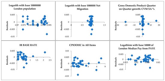
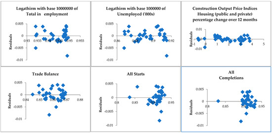
Figure 1. Regression residual plots for model 1: House Price Index Cash purchases.

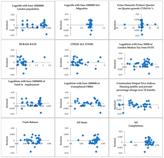
Figure 2. Regression residual plots for model 2: House Price Index Mortgage Purchases.

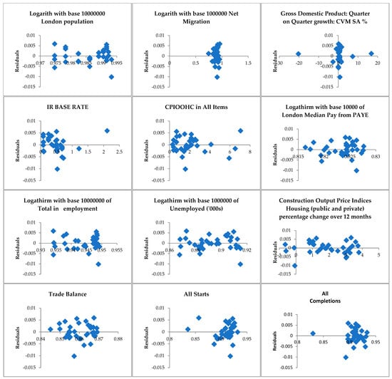
Figure 3. Regression residual plots for model 3: House Price Index New build.

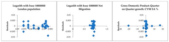
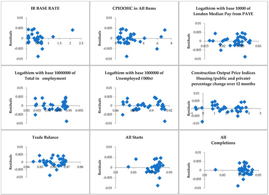
Figure 4. Regression residual plots for model 4: House Price Index in All Property Types.

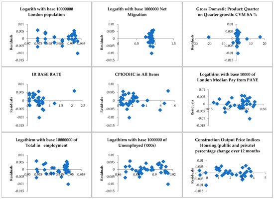
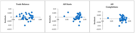
Figure 5. Regression residual plots for model 5: House Price Index First-time buyers.

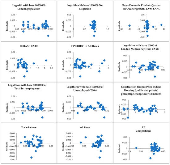
Figure 6. Regression residual plots for model 6: House Price Index Former owner-occupiers.

In order to examine further the effect of interest rate base rates, inflation (consumer price index occupiers’ housing costs), and the construction output price indices housing, they were examined in a further regression analysis as opposed to the HPI in mortgage purchases (log transformed) as shown in model 7 (see Table 2). The results were not found statistically significant and carried a very low R-square and adjusted R-square, as expected, considering their direct impacting on this particular dependent variable. Consequently, this shows adding independent variables improves the model’s goodness of fit (r-square) and the explanation of the variance of the dependent variable is substantially greater, which is consistent with the clusters identified in the net migration and GDP growth residual plots in Figure 1, Figure 2, Figure 3, Figure 4, Figure 5 and Figure 6. In this case, it was found that the interest rate base rate and consumer price index occupiers’ housing costs need other independent variables such as the London population and construction output price indices housing to increase the goodness of fit of the model.

The data results highlight the strong influence that both first- and second-time buyers have on interest rate amendments, while the Brexit migration restrictions have increased the shortage of low- to mid-skilled workers which has increased the time and cost of construction, leading to increased property prices and lowered buyers’ purchasing power. However, the provision of low interest loans and the extension of existing housing schemes such as Help to Buy and Shared Ownership would help more buyers enter the London market; first-time buyers and former owner-occupiers are struggling with inflation, interest rates, and increasing housing costs.

It is noteworthy that the results also have broader Brexit implications covering the international housing markets, including those that hold major financial hubs such as New York, Paris and Hong Kong, such as restrictions in capital flow and investors’ behaviour, which led to them shifting their funds away from the UK due to its economic uncertainty, stricter migration controls, and regulatory changes.

To conclude, the findings are aligned with the fundamentals of real estate economics and urban planning theories. Where supply and demand theories are is visible in the effect that the independent variables of population, interest rates, inflation, construction costs, and net migration have on London property prices.

The urban planning theories are evident through shifting migration in suburban areas and other cities apart from London, which is due to the affordability issues in purchasing a property from certain consumer segments and especially from non-cash buyers and investors.

5. Research Limitations and Further Research

Since Brexit is a relatively recent topic for researchers, its ongoing economic effects in the UK and London may pose a challenge regarding the accuracy of data results; insufficient data and limited previous literature were a challenge in this study, for example. A short-term dataset of 34 observations per variable was collected due to insufficient data on specific time periods. While this prevented the accuracy of the predictions in the models, it reduced overfitting due to capturing a broader variation range, increased the model robustness through outlier minimization, and generally improved the model’s performance giving more reliable results. Monthly data were aggregated to be converted into quarterly data, averaging three months into one quarter to align all data into quarterly data, and this might have deteriorated or weakened the reliability of the results of the study, as researchers suggest, when using this method.

Following the Brexit referendum and the UK’s formal departure from the European Union in January 2020, several regulatory shifts significantly impacted both domestic and international demand in London’s housing market. One of the most notable changes was the end of the EU’s freedom of movement, which introduced stricter visa requirements for EU citizens. This resulted in a decline in low- to mid-skilled migrant labour, particularly in the construction sector, contributing to rising construction costs and delays in housing delivery. Simultaneously, the revised immigration policies favoured high-skilled workers through the new points-based system, potentially shifting the demographic composition of housing demand toward higher-income segments.

Additionally, financial market adjustments included increased scrutiny and compliance for foreign capital flows into UK real estate, especially from jurisdictions previously benefiting from EU regulatory alignment. These changes, combined with heightened geopolitical uncertainty, led to a temporary contraction in foreign investment, particularly from European institutional investors who faced regulatory divergence risks. Capital controls and due diligence requirements were also heightened to align with anti-money laundering (AML) and Know-Your-Customer (KYC) frameworks, increasing transaction complexity for overseas buyers. The imposition of an additional 2% Stamp Duty Land Tax (SDLT) surcharge for non-UK residents in April 2021 further increased acquisition costs for foreign investors, reducing the attractiveness of the London market for some offshore buyers.

Despite these barriers, the long-term appeal of London as a global financial hub preserved a core level of investor interest, particularly among cash buyers seeking stable, high-value assets. However, the combination of tighter regulatory oversight, shifting migration patterns, and rising transaction costs reshaped the market by reducing liquidity, increasing construction timelines, and altering the profile of typical buyers—contributing to the uneven performance observed across different housing market segments in the post-Brexit era.

The data could have been processed through SPPS statistical software, instead of Excel, for enhanced comprehensive and detailed statistical summary output, ease of use, accuracy, and effectiveness. A time series could have been employed for this study for seasonality identification causing housing price cyclical circles, and also long-term trends which aid the process of identifying the long-term effects of Brexit as it smoothes the short-term fluctuations that cause noise—a standard error term.

In addition to the above, there were other exogenous and endogenous factors within the study period which affected house prices, such as COVID-19 and the Suez Canal blockage as found in previous research [37], that deteriorated the housing market, or the UK government policy of a stamp duty holiday that significantly boosted the housing market. These events could be examined further and incorporated deeply for further research in conjunction with Brexit to analyse how major events affect property prices in London and how resilient London’s real estate market is.

Further research on this study period could be employed on other resilient real estate markets, such as New York, to identify how these two cities’ economies interacted with Brexit and their effect on the housing market and prices on a local level (London) along with the spillover effect on a cross-border market level (New York). This could employ a Multi-country VAR model [40] providing insights into the shift in demand of investors in other resilient markets such as those of New York and how the increasing financing costs may block both locals and investors from investing in London.

GDP quarter-on-quarter growth, trade, completed houses, and economic shocks were not found statistically significant in this study. This is further supported by the very low values of correlation between HPIs and GDP quarter-on-quarter growth and all completions, respectively, suggesting almost no correlation, as presented in the correlation matrix (see Table A4), such as in previous predicted findings of an 8% decrease in price with 20k additional house completions, while an increase of GDP had a positive correlation on the NHPI and the increase of completed dwellings (housing supply) was decreasing the HHPI, and a 5.9% increase in housing prices caused by a 1% growth in GDP [3]. There have been studies on GDP growth in similar metropolitan cities, such as the US historical GDP growth effect on UK price appreciation [2,41]. While studies show that house prices changed due to economic shocks like COVID-19, the 1970s oil crises, and the 2008 financial crisis [8], trade was found to affect housing prices in other studies [9]. Therefore, it is vital to further examine this unexplained variation (error term) on the dependent variables, adding more variables such as London property microeconomic factors such as the number of bedrooms, the total property area, covered internal areas, covered verandas, uncovered verandas, the existence of storage and parking, and year of construction, in order to get more comprehensive results. Nevertheless, it is noteworthy that the indexes used in this study differ which may affect the results significantly.

6. Conclusions

This study provides robust empirical evidence on the macroeconomic and demographic determinants of London housing prices during the period spanning Q3 2014 to Q4 2022, with a particular focus on the impact of Brexit. Through the use of multiple regression models across various housing market segments—including cash and mortgage-backed purchases, new builds, and first-time buyers—this research identifies London’s population growth, construction costs, interest rate base rates, and inflation as the most influential variables affecting housing price fluctuations.

Among all variables, population size emerged as the most powerful driver, particularly for mortgage-backed and first-time buyer segments, where a 1% increase in population was associated with a 4–5% rise in house prices. This aligns with the fundamental economic principle that demand-side pressure in a supply-constrained market leads to price escalation. Moreover, cash purchases—largely driven by foreign investors—were found to be more resilient to macroeconomic volatility, suggesting that liquidity-rich buyers play a stabilizing role in high-value markets.

While net migration was not consistently significant across all models, its influence in segments involving cash buyers and former owner-occupiers underscores its importance for investment-driven transactions. The study also confirms that interest rate hikes and rising construction costs substantially hinder affordability for mortgage-dependent buyers, a concern that has intensified in the post-Brexit context amid tighter monetary policy and disrupted supply chains.

The analysis suggests that Brexit has had both direct and indirect effects on the housing market. Directly, it introduced regulatory and fiscal changes—such as new visa rules and the 2% foreign buyer tax—that altered investment incentives. Indirectly, it exacerbated labour shortages in construction and increased economic uncertainty, both of which influenced housing supply and demand dynamics. From a policy standpoint, the findings highlight the need for targeted interventions to improve affordability and market accessibility. These may include expanding affordable housing supply, supporting construction labour through visa adjustments, offering financial assistance to first-time buyers, or introduce value-based recurrent property taxation to prevent affordability challenges and stabilize revenues in response to future market volatility [42], and maintaining transparency to attract responsible foreign investment. Future research should incorporate micro-level property characteristics, explore cross-city comparisons with other global financial centers, and assess the long-term interplay between exogenous shocks (e.g., COVID-19) and structural changes in the UK housing market. By bridging macroeconomic theory with real estate practice, this study contributes valuable insights into the evolving landscape of London’s residential market in the face of geopolitical transformation.

References

- Green, R.K.; Hendershott, P.H. Age, Housing Demand, and Real House Prices. Reg. Sci. Urban Econ. 1996, 26, 465–480. [Google Scholar] [CrossRef]
- Ansell, B.; Adler, D. Brexit and the politics of housing in Britain. Polit. Q. 2019, 90, 105–116. [Google Scholar] [CrossRef]
- Sivitanides, P.S. Macroeconomic drivers of London house prices. J. Prop. Invest. Financ. 2018, 36, 539–551. [Google Scholar] [CrossRef]
- Andrew, M.; Meen, G. House price appreciation, transactions and structural change in the British housing market: A macroeconomic perspective. Real Estate Econ. 2003, 31, 99–116. [Google Scholar] [CrossRef]
- Lindh, T.; Malmberg, B. Demographics and housing demand—What can we learn from residential construction data? J. Popul. Econ. 2008, 21, 521–539. [Google Scholar] [CrossRef]
- Glaeser, E.L.; Gyourko, J. Urban Decline and Durable Housing. J. Polit. Econ. 2005, 113, 345–375. [Google Scholar] [CrossRef]
- Sutton, G.D. Explaining changes in house prices. BIS Q. Rev. 2002, 32, 46–55. [Google Scholar]
- Yoon, J.H.; Nawrot, K.A. Impact of Brexit on G7 properties. AEcon 2022, 54, 6551–6558. [Google Scholar] [CrossRef]
- Dhingra, S.; Sampson, T. Expecting Brexit; CESifo Working Paper Series No. 9541; CESifo: München, Germany, 2022. [Google Scholar]
- Gamble, A. Taking Back Control: The Political Implications of Brexit. In The Politics and Economics of Brexit; Routledge: London, UK, 2021; pp. 127–144. [Google Scholar] [CrossRef]
- Taltavull de La Paz, P.; White, M. The sources of house price change: Identifying liquidity shocks to the housing market. J. Eur. Real Estate Res. 2016, 9, 98–120. [Google Scholar] [CrossRef][Green Version]
- White, M. Cyclical and structural change in the UK housing market. J. Eur. Real Estate Res. 2015, 8, 85–103. [Google Scholar] [CrossRef]
- Hilber, C.A.L.; Vermeulen, W. The Impact of Supply Constraints on House Prices in England. Econ. J. 2014, 126, 358–405. [Google Scholar] [CrossRef]
- Bouchouicha, R.; Ftiti, Z. Real estate markets and the macroeconomy: A dynamic coherence framework. Econ. Model 2012, 29, 1820–1829. [Google Scholar] [CrossRef]
- Bjørnland, H.C.; Jacobsen, D.H. The role of house prices in the monetary policy transmission mechanism in small open economies. J. Financ. Stab. 2010, 6, 218–229. [Google Scholar] [CrossRef]
- Giuliodori, M. The Role of House Prices in The Monetary Transmission Mechanism Across European Countries. Scott. J. Political Econ. 2005, 52, 519–543. [Google Scholar] [CrossRef]
- Rossall Valentine, D. Solving the UK Housing Crisis; The Bow Group: London, UK, 2015. [Google Scholar]
- Goodhart, C.; Hofmann, B. Asset Prices, Financial Conditions, and the Transmission of Monetary Policy. In Proceedings of the Conference on Asset Prices, Exchange Rates, and Monetary Policy, Stanford University, Stanford, CA, USA, 2–3 March 2001. [Google Scholar]
- Muellbauer, J.; Cameron, G. The Housing Market and Regional Commuting and Migration Choices. In CEPR Discussion Paper; No. 1945; CEPR: London, UK, 1998. [Google Scholar]
- Pashardes, P.; Savva, C.S. Factors affecting house prices in Cyprus: 1988-2008. Cyprus Econ. Policy Rev. 2009, 3, 3–25. [Google Scholar]
- Stock, J.H.; Watson, M.W. Vector autoregressions. J. Econ. Perspect. 2001, 15, 101–115. [Google Scholar] [CrossRef]
- Kishor, N.K. Forecasting House Prices: The Role of Fundamentals, Credit Conditions, and Supply Indicators; University Library of Munich: Munich, Germany, 2023; MPRA Paper 116819. [Google Scholar]
- Aljandali, A.; Tatahi, M. Economic and Financial Modelling with EViews: A Guide for Students and Professionals; Springer International Publishing: Cham, Switzerland, 2018; pp. 1–300. [Google Scholar] [CrossRef]
- Box, G.E.; Jenkins, G.M.; Reinsel, G.C.; Ljung, G.M. Time Series Analysis: Forecasting and Control; John Wiley & Sons: Hoboken, NJ, USA, 2015. [Google Scholar]
- Stock, J.H.; Watson, M.W. Chapter 8—Dynamic factor models, factor-augmented vector autoregressions, and structural vector autoregressions in macroeconomics. In Handbook of Macroeconomics; Taylor, J.B., Uhlig, H., Eds.; Elsevier: Amsterdam, The Netherlands, 2016; Volume 2, pp. 415–525. [Google Scholar] [CrossRef]
- Chang, L.; Shi, Y. A Discussion on the Robust Vector Autoregressive Models: Novel Evidence from Safe Haven Assets. Ann. Oper. Res. 2024, 339, 1725–1755. [Google Scholar] [CrossRef]
- Montgomery, D.C.; Peck, E.A.; Vining, G.G. Introduction to Linear Regression Analysis, 5th ed.; Wiley: Hoboken, NJ, USA, 2012. [Google Scholar]
- Miles, J. R-squared, adjusted R-squared. In Encyclopedia of Statistics in Behavioral Science; Wiley: Hoboken, NJ, USA, 2005. [Google Scholar] [CrossRef]
- Chen, Q.; Qi, J. How Much Should We Trust R2 and Adjusted R2: Evidence from Regressions in Top Economics Journals and Monte Carlo Simulations. J. Appl. Econ. 2023, 26, 2207326. [Google Scholar] [CrossRef]
- Asuero, A.G.; Sayago, A.; González, A.G. The correlation coefficient: An overview. Crit. Rev. Anal. Chem. 2006, 36, 41–59. [Google Scholar] [CrossRef]
- Sedgwick, P. Pearson’s correlation coefficient. BMJ 2012, 345, e4483. [Google Scholar] [CrossRef]
- Kutner, M.H.; Nachtsheim, C.J.; Neter, J.; Li, W. Applied Linear Statistical Models, 5th ed.; McGraw-Hill/Irwin: New York, NY, USA, 2005. [Google Scholar]
- Montgomery, D.C.; Runger, G.C. Applied Statistics and Probability for Engineers, 6th ed.; Wiley: Hoboken, NJ, USA, 2014. [Google Scholar]
- Stephens, M.; Perry, J.; Wilcox, S.; Williams, P.; Young, G. 2018 UK Housing Review: Autumn Briefing Paper; Chartered Institute of Housing: Coventry, UK, 2018. [Google Scholar]
- Di Iasio, V.; Wahba, J. Expecting Brexit and UK Migration: Should I Go? Eur. Econ. Rev. 2023, 157, 104484. [Google Scholar] [CrossRef]
- Savva, C.S. Factors affecting housing prices: International evidence. Cyprus Econ. Policy Rev. 2018, 12, 87–96. [Google Scholar]
- Malik, A.; Adekoya, O.D.; Ajonbadi, H.A.; Jimoh, I. Investigating the Potential Economic Impact of Brexit Decisions on Business Performance in the United Kingdom: A Case Study of the UK Construction Industry. Int. J. Manag. Account. Econ. 2019, 6, 347–367. [Google Scholar]
- Broadbent, B.; Di Pace, F.; Drechsel, T.; Harrison, R.; Tenreyro, S. The Brexit Vote, Productivity Growth, and Macroeconomic Adjustments in the United Kingdom; Bank of England: London, UK, 2019; Available online: https://www.bankofengland.co.uk/-/media/boe/files/external-mpc-discussion-paper/2019/the-brexit-vote-productivity-growth-and-macroeconomic-adjustments-in-the-united-kingdom.pdf (accessed on 6 April 2024).
- Breinlich, H.; Leromain, E.; Novy, D.; Sampson, T. Exchange Rates and Consumer Prices: Evidence from Brexit; CEP Discussion Paper No 1667; Centre for Economic Performance, LSE: London, UK, 2019. [Google Scholar]
- Canova, F.; Ciccarelli, M. Estimating Multicountry VAR Models. Int. Econ. Rev. 2009, 50, 929–959. [Google Scholar] [CrossRef]
- Himmelberg, C.; Mayer, C.; Sinai, T. Assessing High House Prices: Bubbles, Fundamentals and Misperceptions. J. Econ. Perspmect. 2005, 19, 67–92. [Google Scholar] [CrossRef]
- Grover, R.; Walacik, M. Property valuation and taxation for fiscal sustainability—Lessons for Poland. Real Estate Manag. Valuat. 2019, 27, 35–48. [Google Scholar] [CrossRef]
Disclaimer/Publisher’s Note: The statements, opinions and data contained in all publications are solely those of the individual author(s) and contributor(s) and not of MDPI and/or the editor(s). MDPI and/or the editor(s) disclaim responsibility for any injury to people or property resulting from any ideas, methods, instructions or products referred to in the content. |
© 2025 by the authors. Licensee MDPI, Basel, Switzerland. This article is an open access article distributed under the terms and conditions of the Creative Commons Attribution (CC BY) license (https://creativecommons.org/licenses/by/4.0/).