Automated Weld Defect Detection in Industrial Ultrasonic B-Scan Images Using Deep Learning

Abstract

Automated ultrasonic testing (AUT) is a nondestructive testing (NDT) method widely employed in industries that hold substantial economic importance. To ensure accurate inspections of exclusive AUT data, expert operators invest considerable effort and time. While artificial intelligence (AI)-assisted tools, utilizing deep learning models trained on extensive in-laboratory B-scan images, whether they are augmented or synthetically generated, have demonstrated promising performance for automated ultrasonic interpretation, ongoing efforts are needed to enhance their accuracy and applicability. This is possible through the evaluation of their performance with experimental ultrasonic data. In this study, we introduced a real-world ultrasonic B-scan image dataset generated from proprietary recorded AUT data during industrial automated girth weld inspection in oil and gas pipelines. The goal of inspection in our dataset was detecting a common type of defect called lack of fusion (LOF). We experimentally evaluated deep learning models for automatic weld defect detection using this dataset. Our assessment covers the baseline performance of state-of-the-art (SOTA) models, including transformer-based models (DETR and Deformable DETR) and YOLOv8. Their flaw detection performance in ultrasonic B-scan images has not been reported before. The results show that, without heavy augmentations or architecture customization, YOLOv8 outperforms the other models with an F1 score of 0.814 on our test set.

1. Introduction

Ultrasonic testing (UT) is a nondestructive testing (NDT) technique used for inspecting components and structures to ensure their integrity and quality. The advantage of employing NDT methods is that the structures can be inspected without interruptions in their daily functions, offering a nonintrusive means of assessing structural health. NDT is widely used in safety-critical industries such as aerospace, automotive, and oil and gas, where the reliability of structures plays an important role.To enhance the overall confidence and efficiency of the inspection process, researchers are increasingly exploring new techniques such as optimizing laser-induced arrays for defect detection [1], implementing automated computer-aided inspection for real-time defect detection in laser-welded blanks [2], etc. In comparison to other NDT methods, UT boasts a long history of effectively detecting subsurface [3] and small flaws [4]. In UT, a transducer placed on the surface emits ultrasound waves through the material. By analyzing the waves reflected back to the transducer, corrosion and flaws that occurred during manufacturing, welding, or other processes can be detected and assessed.

Automated ultrasonic testing (AUT) utilizes automated systems mounted around the structure, performing precise and rapid inspection with phased array probes. In phased array technology, each element in the array is pulsed and delayed independently, creating a varied range of beam angles and focal points for the comprehensive examination of materials. Presently, AUT inspection entails an analysis of an ever-expanding volume of acquired data by human operators. The responsibilities during AUT inspections encompass a range of tasks for operators. These include positioning the inspection head around the structure, conducting inspections, interpreting data, recording results, and making decisions as to whether to accept or reject the scanned profiles. These intricate, sequential tasks, coupled with the multitude of scans requiring inspection, could compromise accuracy and extend the time needed for UT interpretations.

In UT, data are often recorded in the form of A-scans, B-scans, and C-scans. B-scans, which visualize more detailed information about the inspected material, have captured considerable interest within the field of UT. After the introduction of ImageNet [5] in the computer vision community, substantial efforts have been directed toward harnessing deep-learning-based algorithms to tackle challenges in downstream tasks, especially in the interpretation of ultrasonic B-scan images.

In [6], the authors conducted experiments using both conventional algorithms, such as flaw classifiers based on hand-crafted features and statistical techniques, and machine-learning-based methods, including convolutional neural networks (CNNs), to classify defects in images obtained from the laser-generated imaging of ultrasonic wave propagation [7,8] on stainless-steel plates. In their subsequent work [9], first, they released the first publicly available dataset for ultrasonic inspection named USimgAIST [10], consisting of 7004 images with both normal cases and defective cases from 18 stainless steel plates including drill holes and slits flaws. Second, they trained multiple SOTA deep CNNs on their dataset to benchmark deep learning models for automatic ultrasonic image interpretation. In [11], a reinforcement-learning-based neural architecture search neural network (RL-NAS NN) was utilized to automatically implement the optimal CNN-based architecture for classifying defects on the USimgAIST dataset. All previous methods, despite proposing a novel idea for ultrasonic image interpretation, suffer from an inability to detect the size and the location of the defects.

The first application of SOTA CNN-based object detectors for AUT was implemented in [12]. They fine-tuned YOLOv3 [13] and SSD [14] on their dataset containing 490 grayscale B-scan images with 1562 annotations using heavy augmentation methods. Another SOTA one-stage object detector, EfficientDet-D0 [15], using custom-calculated anchors, was exploited in [16] to detect flaws on their in-house dataset containing 4147 B-scan images that were artificially flawed. DefectDet [17], a novel deep learning architecture, was created by replacing the default backbone of EfficientDet with a lightweight encoder–decoder-based feature extractor and a custom detection head for detecting objects with extreme aspect ratios by shifting the input to the biFPN block in the architecture. Despite the advancements in automated defect detection techniques, the reliability of these deep learning models heavily relies on a large and well-distributed dataset.

Generating a substantial amount of ultrasonic B-scan data is time-consuming and costly. Therefore, many studies on classifying and localizing flaws in ultrasonic B-scan images have often relied on in-laboratory images from inspected test specimens under controlled conditions or a limited amount of real-world UT image data that are multiplied using techniques such as image augmentation or synthetic data generation to supply data-hungry deep neural networks (DNNs) for training. Moreover, to build a dataset with a variety of flaws, researchers have commonly introduced artificial defects into images or have intentionally created flaws on test specimens.

In [18], the authors employed extensive data augmentation for their virtually flawed ultrasonic data [19] with varying backgrounds to create their 10,000-size image dataset. With the advent of AI, instead of relying solely on augmentation, more reliable methods for extending the number of training inputs have emerged. In [20], the authors proposed two generative-adversarial-based networks, DetectionGAN [21], and a modified SPADE GAN [22] for generating synthetic B-scan images that are hardly indistinguishable from the real ones for UT operators. Despite the significant advancements made in the field of AUT, the lack of experiments conducted on datasets derived from extreme environments is apparent.

It is evident that the distribution of data obtained from in-laboratory experiments may differ from that of onshore inspections. This discrepancy could pose a significant concern for applications where deep-learning-based models play a role in the decision-making process for ultrasonic interpretation. In this paper, we introduce a proprietary B-scan image dataset that we generated from recorded reports of onshore automated girth weld inspections of oil and gas pipelines in extreme conditions acquired by UT experts. Additionally, the type of flaw present in our dataset is a lack of fusion (LOF), a common flaw in automated girth welding. We believe that this is the first time in the literature that ultrasonic B-scan images captured from industrial environments with real flaws, specifically LOF, are utilized for fine-tuning deep learning algorithms. 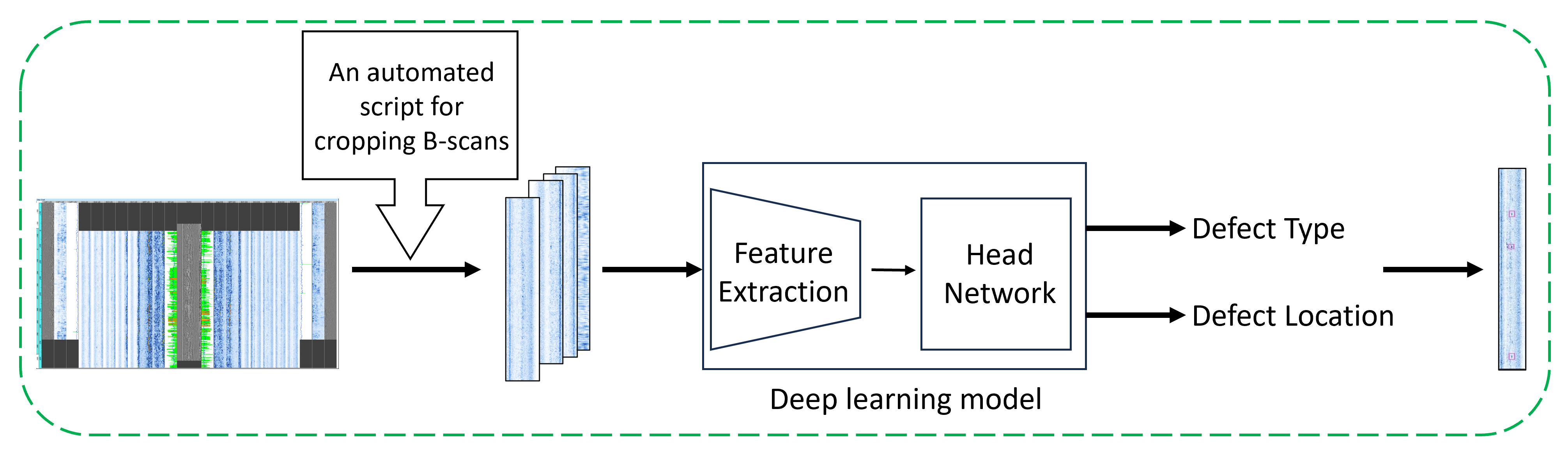We aimed to investigate the performance of SOTA deep-learning-based models without any additional synthetic data or modification to the architectures to see their baseline performance on industrial B-scan images.We illustrate our work in Figure 1, where an expert human operator performs automated ultrasonic inspections onshore. Once the inspection is completed, the data are captured and stored using acquisition software. Subsequently, the inspected data are processed and fed into a neural-network-based flaw detector, which analyzes the data to identify potential flaws. Finally, the expert human operator reviews and validates the results, providing a crucial check to correct any missed or incorrect detections.

The contributions of this work are as follows:

• We introduce a proprietary industrial ultrasonic B-scan images dataset that is generated from recorded AUT inspections performed by human inspectors during onshore oil and gas girth weld inspections.
• In addition to the B-scan dataset, genuine flaws that usually occur during automated girth welding, such as LOF, are introduced and investigated.
• We fine-tune and evaluate SOTA models, such as transformer-based architectures (DETR and Deformable DETR) and YOLOv8, on industrial ultrasonic B-scan images.

The remainder of this article is organized as follows: Section 2 provides details on dataset preparation and properties. Section 3 explains the implementation, training, and evaluation processes of several experiments. Section 4 compares the performance of several SOTA models on our B-scan dataset. Finally, Section 5 concludes this paper and presents our work’s limitations and future studies.

2. Dataset

2.1. Dataset Description

We have created a dataset of Ultrasonic B-scan images from weld inspection data acquired by UT experts with automated girth weld inspection system utilizing phased array technology for inspecting oil and gas pipeline. The inspection system utilizes the zone discrimination technique for weld inspection. In this approach, each weld is divided into a few vertical zones, each having a specific beam for inspection. Multiple beams travel around the pipe in a single linear movement. Zone discrimination divides the weld into three main regions: The Cap region, Body region, and Root region. The Cap and Body regions include zones such as Fill 1 and Fill 2, respectively. The Root region includes Hot pass 2, Hot pass 1, LCP, and Root. Figure 2 represents the three regions in the Zone discrimination technique. In our dataset, the weld type is J-bevels, and the weld defect class is lack of fusion (LOF), which is the most common defect in automated girth welding.

2.2. Dataset Preparation

We created our dataset using 87 proprietary weld inspection records recorded by UT experts with the inspection system during onshore oil and gas pipeline girth weld inspections. We were not involved in the inspection process; we only collected B-scan images from the proprietary weld inspection data provided to us by UT experts. Each recorded weld datum includes a 1920 × 1080 image containing multiple strip charts representing the output of the channels of the phased array probes used for AUT. The strip charts also provide views of the downstream and upstream phased array probes, as well as each weld zone that each channel represents. Moreover, each recorded weld datum contains a table filled out by human operators including the type, size, and location of the detected flaws on each strip chart image. Human operators also annotated the exact location of each flaw in each related strip chart with a bounding box. The recorded data include both the raw inspected weld data and the interpreted weld data. From the weld inspection datasets, we collected 359 B-scan strip chart images. The distribution of our B-scan dataset covers Fill 1, Hot pass 1, and Hot pass 2 zones. Figure 3 represents the 1920 × 1080 image from one of the recorded weld data files.

Each 1920 × 1080 image contains 23 or 27 strip charts. These strip chats can display A-scan, B-scan, and TOFD ultrasonic images. In this study, our primary focus was on the B-scan images within the strip charts. Manually cropping each of these strip charts from the main image is time-consuming and prone to inaccuracy. To address this, we developed an automated Python script for the task. The script crops the strip charts from the main image automatically. We collected 359 B-scan images from the main images. We used DarkMark (https://github.com/stephanecharette/DarkMark, accessed on 15 August 2023, v1.8.11-1, Stéphane Charette, West Kelowna, BC, Canada) software to annotate flaws on the raw B-scan images based on human operator interpretations. For training, and evaluation of deep learning models, we divided the dataset into training, validation, and test sets. In

Table 1. Training, validation, test set image quantity.

Split	Images W Annot.	Images W/o Annot.	Total Images	Total Annot.
Training	95	243	338	182
Validation	10	0	10	16
Test	11	0	11	31

, we provide details about the quantity of images, annotations, and negative samples in each set. Our dataset contains a total of 229 LOF annotations across B-scan images. Figure 4 presents 7 B-scan images and 10 LOF annotations from the training set.

In the final subsection, we analyze our B-scan dataset images to gain valuable insights. We believe that this information helped us with fine-tuning and interpreting the utilized deep-learning-based model more effectively.

2.3. Dataset Properties

The primary inspiration for this section of the study comes from https://deci.ai/course/profiling-computer-vision-datasets-overview (accessed on 17 November 2023). We only used their descriptions for image analysis to implement them based on our B-scan dataset. We did not use their Python package for generating our figures in this article.

2.3.1. Image Dataset Analysis

In this section of this study, our objective was to analyze the images themselves, disregarding the bounding boxes used for defect annotations. We analyzed these images based on their brightness distribution, width and height distribution, and mean and standard deviation (STD) of the pixels in the images. To begin, we focused on brightness distribution. For brightness analysis, we converted each image from the RGB to the LAB color space and calculated the average of the lightness (L) component. The resulting brightness distribution for all three sets is plotted in a kernel density (KDE) plot in Figure 5, revealing that the brightness distribution in the validation and test sets was mostly consistent with that of the training set images.

Next, we examined the dimensions distribution of all images. Figure 6 shows the number of images with specific width or height sizes for the three sets, demonstrating that the resolutions of images from the validation and test sets are included in the test set.

The other properties we calculated for our dataset were mean (Used “Mean pixels for normaliztion.ipynb” script from this repo https://github.com/iDataVisualizationLab/roaddamagedetector (accessed on 26 January 2024) for pixel mean calculations) and STD of pixels over three image channels including red, green, and blue. These properties could be helpful for more customization of the deep-learning-based object detector model, which was pretrained on the ImageNet [23] and COCO [24] dataset.

Table 2. Mean and STD of pixels in our dataset in RGB format.

Split	Mean	STD
Training	[214.52, 230.39, 247.45]	[32.78, 23.22, 12.52]
Validation	[214.15, 230.02, 247.26]	[35.03, 24.86, 12.75]
Test	[211.56, 228.64, 246.99]	[33.21, 23.26, 12.21]

includes the mean and STD of pixels for the images in each set in our dataset.

In the next section, we analyze the bounding box features based on our dataset.

2.3.2. Bounding Box Analysis

For the analysis of the implemented bounding boxes for annotations, we discuss the drawing bounding boxes based on the area of each defect as a percentage of the total B-scan image, their counts in each image, and the spatial distribution of defects in the images in our dataset. We performed these analyses for our training, validation, and test sets.

To analyze the distribution of bounding box area for each image in each set, the area of each bounding box was calculated as a percentage of the total B-scan image area. Figure 7 represents the LOF defects’ area distribution in our dataset. Based on the plots, it is noticeable that we faced the challenge of detecting small defects in our B-scan image dataset. The minimum and maximum square roots of the bounding box area (anchor box size) in our training set were almost 16 and 32, respectively.

The bounding boxes’ height/width ratio distribution (anchor box ratio) is represented in Figure 8. It indicates the anchor box ratio for training set was mainly focused in the middle of the distribution graph including 1.2, 1.4, and 1.7.

Moreover, we analyzed the bounding boxes based on their location in each image. In Figure 9, the defects are distributed throughout the images in each set. This can be advantageous for training a model with more generalization ability based on the consistently distributed defects in our dataset.

Finally, Figure 10 demonstrates the number of bounding boxes appearing in each set of images. Through this analysis, we gained an idea of the maximum number of defects that a model should detect in an image based on our dataset.

3. Experimental Results

In this section, we first introduce the models selected for our experiments. Then, we delve into the configurations and hyperparameters that were set manually for each model during training and evaluation. Finally, we compare the performance of these models on our validation and test sets.

We selected five SOTA object detectors to fine-tune them on our task. The models for our experiments included RetinaNet [25], DETR [26], Deformable DETR [27], YOLOv5u [28], and YOLOv8 [29]. These models mainly comprise CNN-based (RetinaNet, YOLOv5u, and YOLOv8) and transformer-based (DETR and Deformable DETR) object detectors. The reasoning behind choosing these models is that, first, we included RetinaNet and YOLOv5, which have been studied in previous works [16,17] on B-scan images, to evaluate their performance on our dataset. Moreover, the performance of end-to-end transformer-based object detectors (DETR and Deformable DETR) and recent CNN-based architectures (YOLOv8) has not been previously investigated on B-scan images by the research community. Therefore, the aim of the selection of these diverse architectures was to broaden our understanding of the performance and impact of different types of deep-learning-based object detectors for the UT flaw detection task.

In the following, we elaborate on the configurations and hyperparameters that we manually set for each model during the training and evaluation stages. The main hyperparameters we manually set were the learning rate, input image size to the networks, and the numbers of iterations and epochs. The rationale behind choosing these was to set them based on the properties of our image dataset. Any configurations and hyperparameters not explicitly mentioned were kept consistent with the choices made by the model developers during the pretraining phase. Our objective in this step was to maintain most of the settings used for pretraining the models, aiming to establish the preliminary results of these models on our dataset as the baseline. All models were fine-tuned and evaluated on a single Nvidia A100 40 GB GPU with Cuda 11.8, torch 2.1.2, and torchvision 0.16.2 [30]. To enhance the repeatability of the results across different hyperparameters, we set the random seed to 42 for more deterministic random initializations. Notably, we chose not to train these models from scratch, as discussed in [31], to avoid unnecessarily prolonging the training process without significant improvements in model performance and due to the absence of a sufficiently large dataset for pretraining. Figure 11 represents the streamline through which B-scans passed to be analyzed for potential defects.

3.1. RetinaNet

RetinaNet is a CNN-based single-stage detector that employs a novel loss function called focal loss to address the class imbalance problem during training. One of the key features of RetinaNet is its ability to detect objects across a wide range of scales by using feature pyramid networks [32] and anchors of multiple scales and aspect ratios. We utilized its implementation on Detectron2 [33] with an ImageNet-pretrained ResNet-50 [34] backbone. The initial configuration change involved enabling the model to train on negative samples and avoiding the filtering of empty samples We set _C.DATALOADER.FILTER_EMPTY_ANNOTATIONS to False in detectron2/config/defaults.py and filter_empty argument of get_detection_datasets_dicts to False in detectron2/data/build.py). Flaws in B-scan images can be easily misinterpreted as background due to the complexity of the images, even by humans. By doing so, we allow the model to learn features from backgrounds with nonexistent flaws. We retained the default implemented image augmentation methods for the training, validation, and test sets. For the training set, scale augmentation was applied, resizing the input images so that the shortest side was at least 640 and at most 800 pixels, while the longest side was at most 1333 pixels. In addition, a random horizontal flip with a probability of 0.5 was applied to the training set images. For evaluation on the validation and test sets, images were resized to 800 × 1333 using scale augmentation. The total batch size was set to 64, and training utilized stochastic gradient descent (SGD) [35] with a learning rate of 1 × 10 ${ }^{-4}$ and a weight decay of 0. The training ran for 5000 iterations. The learning rate scheduler increased the initial learning rate from 3 × 10${ }^{-5}$ to 1 × 10${ }^{-4}$ linearly in the first 100 iterations and then maintained the learning rate at 1 × 10${ }^{-4}$ for the next 3200 iterations. Subsequently, the learning rate decayed by a factor of 0.1 in the next 1100 iterations. Finally, the training continued for the last 600 iterations with a learning rate of 1 × 10${ }^{-6}$. To prevent overfitting, we monitored both training and validation loss (with the help of this github repo: https://github.com/ravijo/detectron2_tutorial, accessed on 11 December 2023), we logged validation loss). The Detectron2 platform logged validation loss, applying the same implemented image augmentations for the training set for the validation set. Additionally, the best checkpoint hook with the AP50 metric was incorporated into the training script to track the best model with improved AP50 results on the validation set every 50 iterations. We selected the model with the highest AP50 performance at iteration 1450, before the model started overfitting.

3.2. End-to-End Transformer-Based Object Detectors

For these two models, there are common tuned configurations, which we discuss before addressing the hyperparameters specific to each model separately in their respective sections.

We fine-tuned two transformer-based object detectors, including DETR and Deformable DETR, on our B-scan dataset using their implementations on Detrex [36] codebase based on Detectron2. This framework facilitates the comparison of the performance among different DETR-based models. Both models exploit the ImageNet-pretrained ResNet-50 as their backbone. We exclusively applied the same image augmentation technique to all three image sets, involving rescaling to 96 × 1152 through scale augmentation. Additionally, both models were trained on both negative and positive samples by disabling the filtering of empty samples. The total batch size was set to 64, and training was optimized with AdamW [37], setting the base learning rate to 1 × 10${ }^{-5}$ (in the DETR paper [26], the base learning rate is referred to as the transformer’s learning rate), B1 = 0.9, B2 = 0.999 with no weight decay, keeping the learning rate constant during training. Similar to RetinaNet on Detectron2, we incorporated the best check point hook to save the model with the highest AP50 performance on validation set every 50 iterations. We also monitored training and validation loss to prevent overfitting. For DETR, the training ran for 10,000 iterations, while for Deformable DETR, it was 2000 iterations. We did not use the gradient clipping and expotional moving average (ema) configurations available in the Detrex codebase in our experiments.

3.2.1. DETR

The DETR model is the first end-to-end object detector that uses a transformer architecture [38], departing from the traditional convolutional approach. It treats object detection as a direct set-to-set prediction problem, where a set of object queries attends to the encoded image and outputs a set of predictions in parallel. A key feature of DETR is its simplicity and scalability, as it does not use hand-crafted components like anchor boxes or nonmaximum suppression (NMS). We fine-tuned two different implementations of DETR, namely, DETR-R50 and DETR-DC5-R50. The former is DETR with ResNet-50, while the latter involves DETR with increased feature resolution, which is achieved by adding dilation to the last stage of the backbone and removing a stride from the first convolution of this stage (dilated C5 stage) [26]. The number of object queries was set to 100, which is the default value for DETR. Additionally, the learning rate for the backbone, following the default DETR implementation, was 1 × 10${ }^{-5}$. For DETR, the model with the highest AP50 was achieved at the 8100th iteration, and for DETR-DC5, the best AP50 was attained at iteration 5350.

3.2.2. Deformable-DETR

Deformable DETR is an extension of the DETR model, introducing deformable attention modules that enable attention to a small set of key sampling points around a reference point. This deformable attention mechanism enhances the performance on object detection tasks, particularly for objects with irregular shapes or occlusions, while maintaining the end-to-end simplicity of the original DETR architecture. We fine-tuned three different variants of Deformable DETR, including Deformable DETR-Res50 (DDR50), DDR50 with box refinement, and the two-stage DDR50 with box refinement. The box refinement is an iterative bounding box refinement aimed at improving detection performance. In the two-stage edition, region proposals are generated by a variant of Deformable DETR in the first stage. Then, by feeding the generated proposals to the decoder as object queries for further refinement, the two-stage Deformable DETR is formed [27]. For the number of object queries and backbone learning rate, we followed the Detrex implementations (in the original implementation [27], the number of object queries is 300, the base learning rate is 2 × 10${ }^{-4}$, and the learning rates for the backbone, reference points, and sampling offset are set to 2 × 10${ }^{-5}$. In the Detrex implementation, the backbone learning rate is 1 × 10${ }^{-5}$, while the learning rates for the sampling offsets and reference points are set to be the same as the base learning rate. For our experiment, the base learning rate was configured to 1.0 × 10${ }^{-5}$) by setting it to 300 and 1 × 10${ }^{-5}$, separately. We identified the best model based on the AP50 performance of the three variants of DDR50 at iterations 1600, 700, and 1100.

3.3. YOLO Family

To fine-tune YOLOv5u and YOLOv8, we used their official implementation by Ultralytics. The only parameter we considered in our experiments was the patience parameter, which is for early stopping of training if no improvement is observed in the evaluation on the validation set based on the AP50 metric. We repeated each model’s fine-tuning process with five patience levels [50, 100, 150, 180, 200, 250] and selected the fine-tuned model with the highest mAP50 on the validation set. We set the input image size parameter (imgsz) to 1024. Moreover, the training for both YOLO models and their variants in our experiments ran with the SGD optimizer (learning rate = 0.01, momentum = 0.9, and no weight decay). We did not add any predefined image augmentation techniques to the model, and the default implemented augmentation methods by Ultralytics used for the model, e.g., online imagespace and colorspace augmentations (discussed in https://github.com/ultralytics/yolov5/discussions/10469, accessed on 15 December 2023). In the following, we discuss which variants of each model we chose for our experiments.

3.3.1. YOLOv5u

In general, YOLOv5 builds upon previous versions of the CNN-based You Only Look Once (YOLO) [39] model. It employs several novel techniques such as mosaic data augmentation, self-adversarial training, and adaptive anchors to improve performance. We used the nano edition of YOLOV5u, which is the optimized implementation of the original YOLOV5, benefiting from an anchor-free detection head inspired by YOLOv8. In our experiments, we referred to them as YOLOv5nu and YOLOV5n6u. The former was pretrained on input images with a size of 640 × 640, and the latter with 1280 × 1280. The best weight for YOLOv5nu occurred after 308 epochs with a patience level of 180. For YOLOv5n6u, it occurred after 219 epochs with a patience level of 180.

3.3.2. YOLOv8

YOLOv8 features an anchor-free detection head and optimizes the accuracy–speed trade-off by introducing several novel convolutional-based modules based on the YOLOv5 architecture (For more details, please refer to https://github.com/ultralytics/ultralytics/issues/189, accessed on 14 May 2024) [29,40]. To fine-tune, we used its nano and small variants, YOLOv8n and YOLOv8s. The former’s best weight was captured after 196 epochs with a patience level 100. For the latter, it occurred after 139 epochs with a patience level of 50.

3.4. Evaluation

All fine-tuned models were evaluated on our validation and test sets. Three parameters, including true positive (TP), false negative (FN), and false positive (FP), were calculated for the images in each set. The number of flaws available in the images that are correctly identified by a model is called true positive (TP). The flaws that the model fails to identify are false negatives (FNs). False positive (FP) occurs when the model mistakenly identifies a flaw that is not actually present in the image. Based on these parameters, accuracy, precision, recall, and F1 score were calculated to evaluate the performance of the models using

$$\mathrm{F}1\mathrm{score}=2·\frac{\mathrm{Precision}·\mathrm{Recall}}{\mathrm{Precision}+\mathrm{Recall}}$$

(1)

where

$$\mathrm{Accuracy}=\frac{TP}{TP+FP+FN};\mathrm{Precision}=\frac{TP}{TP+FP};\mathrm{Recall}=\frac{TP}{TP+FN}$$

(2)

The metrics we used for our evaluations were primarily those employed in previous works [9,41,42] for assessing deep-learning-based defect detectors on their respective datasets. Before the calculations of TPs, FPs, and FNs in the evaluation stage, we applied two postprocessing steps to the predictions of each model. First, we considered a threshold value for the confidence (score) property of each prediction. Predictions with a confidence less than the determined threshold value were ignored. The thresholds were not equal across the models and were selected from a range of [0, 1.0] with a step of 0.05 based on each model’s best performance in the accuracy metric (To calculate the TPs, FPs, and FNs with different confidence thresholds for YOLO families, we used the scripts from [43] (https://github.com/Cartucho/mAP, accessed on 10 January 2024). In

Table 3. Comparison the performance of the SOTA models on the detection of the lack of fusion (LOF) flaw on both validation and test sets. The top performance is highlighted in bold, and the second-best is indicated by underline.

		Validation Set								Test Set
Model	Params	C.T.	TP	FP	FN	ACC	P	R	F1	C.T.	TP	FP	FN	ACC	P	R	F1
RetinaNet-Res50	34 M	0.35	14	5	2	0.667	0.737	0.875	0.800	0.30	21	17	10	0.438	0.553	0.677	0.609
DETR-Res50	41 M	0.80	12	4	4	0.600	0.750	0.750	0.750	0.80	18	8	13	0.462	0.692	0.581	0.632
DETR-DC5-Res50	41 M	0.75	10	7	6	0.435	0.588	0.625	0.606	0.70	17	9	14	0.425	0.654	0.548	0.596
Deformable DETR-Res50	40 M	0.35	12	3	4	0.632	0.800	0.750	0.774	0.45	17	3	14	0.500	0.850	0.548	0.667
+bbox refinement	40 M	0.35	13	3	3	0.684	0.813	0.813	0.813	0.20	16	10	15	0.390	0.615	0.516	0.561
++two-stage	40 M	0.10	15	5	1	0.714	0.750	0.938	0.833	0.15	21	7	10	0.553	0.750	0.677	0.712
YOLOv5nu	2.6 M	0.50	13	4	3	0.650	0.765	0.813	0.788	0.15	23	10	8	0.561	0.697	0.742	0.719
YOLOv5n6u	4.3 M	0.50	13	3	3	0.684	0.813	0.813	0.813	0.15	26	11	5	0.619	0.703	0.839	0.765
YOLOv8n	3.2 M	0.40	15	2	1	0.833	0.882	0.938	0.909	0.35	24	4	7	0.686	0.857	0.774	0.814
YOLOv8s	11.2 M	0.55	11	1	5	0.647	0.917	0.688	0.786	0.40	20	3	11	0.588	0.870	0.645	0.741

, the column “C.T.” under each image set represents the selected confidence threshold (C.T.) for that model, indicating the model showing the best performance based on accuracy among the observed thresholds. Additionally, a model prediction was considered a TP when the intersection of the ground truth box and the predicted box was at least a 0.5 intersection over the area of the union of the two mentioned boxes, which is called intersection over union (IOU). In the current stage of our work, after each model made its predictions, in cases of missed or incorrect flaw detections, the predictions were evaluated by UT human experts to finalize the results.

4. Results and Discussion

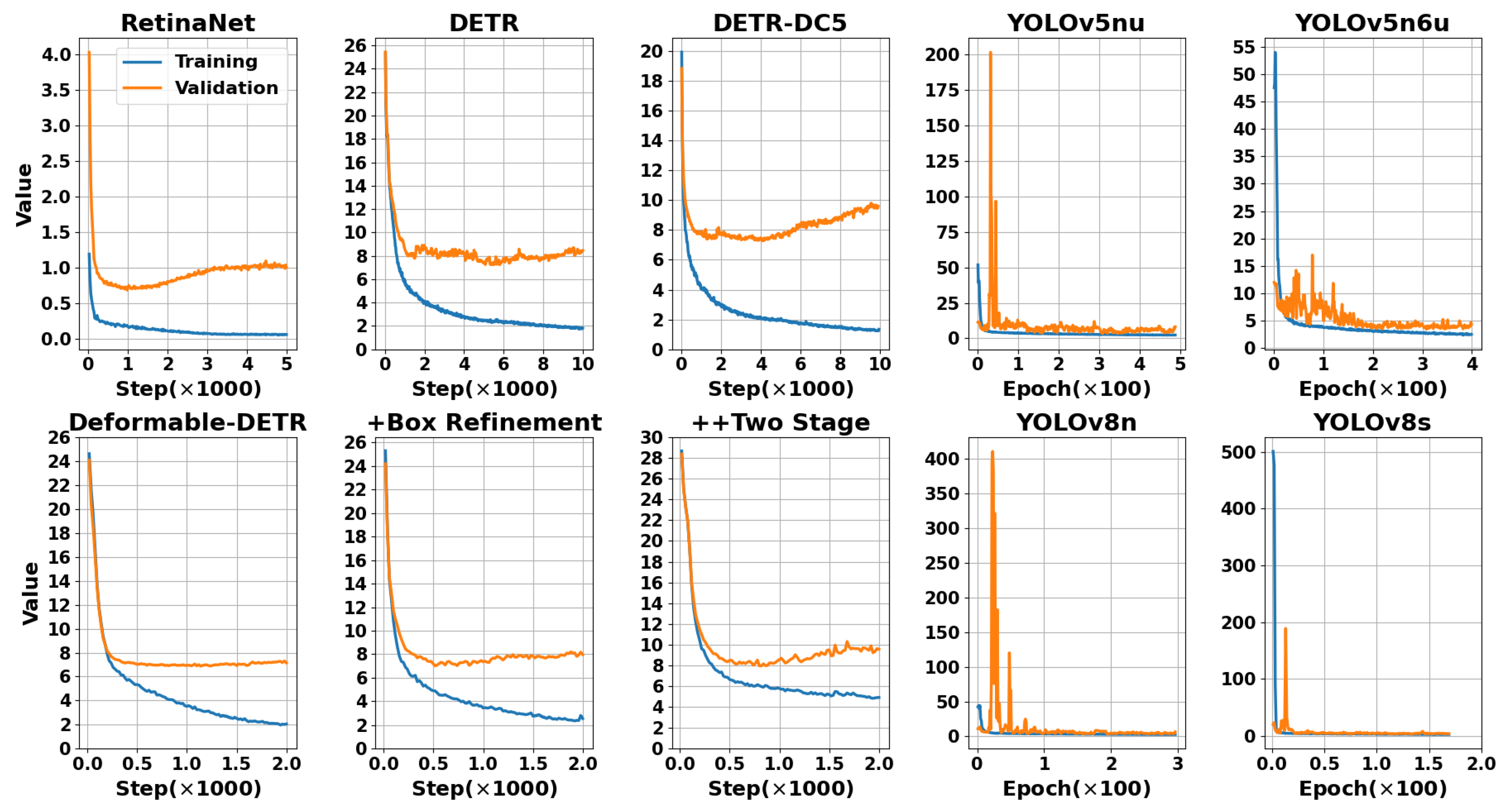
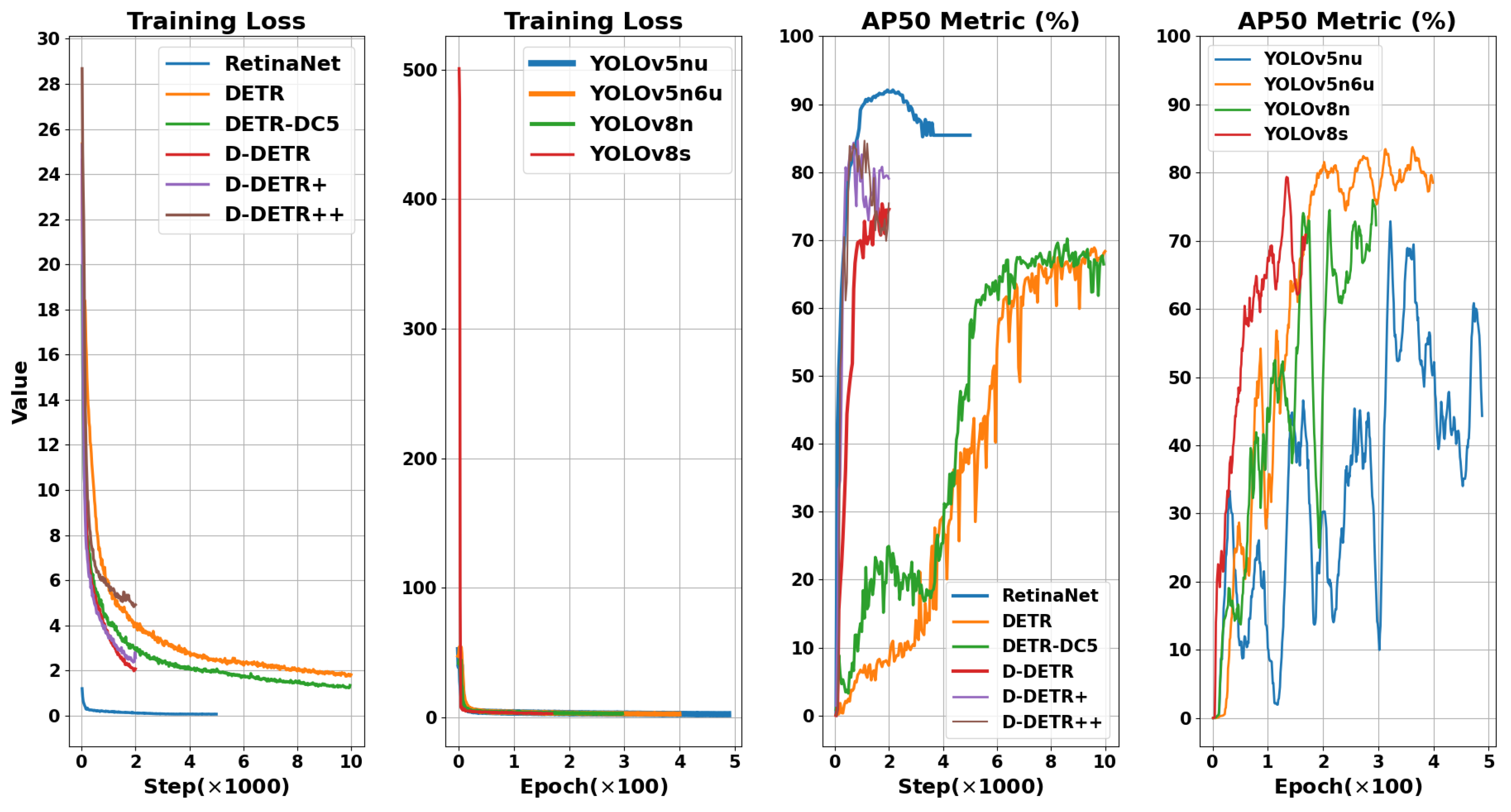
To demonstrate the performance and learning capabilities of the fine-tuned models, we compare their performance on the training set and validation set with their loss plots in Figure 12. To ensure a fair comparison, the term ‘loss’ refers to the total loss for each model. For RetinaNet, the total loss includes class loss and bounding box regression loss; for DETR-based models, it includes class loss, bounding box loss, and GIoUs loss; for YOLO families, it includes class loss, bounding box loss, and directional feature learning (DFL) loss. Additionally, in Figure 13, we compare the training loss and AP50 performance for the fine-tuned models. Since RetinaNet and DETR-based models are iteration-based, while YOLO families are epoch-based, we compared them separately.

Based on the evaluation metrics discussed in the previous section, Table 3 presents the results of each fine-tuned model on both the validation and test sets. Among the evaluated models, YOLOv8n outperformed the others in terms of F1 score on the test set. This metric indicated a balanced performance in precision and recall, suggesting robust minimization of FPs and FNs. For the recall metric, YOLOv5n6u surpassed YOLOv8n, with 8.40% better performance. Recall measured how well a model avoided missing flaws. Regarding the number of TPs, YOLOv5n6u had the highest count on the test set. Moreover, in terms of precision, YOLOv8s outperformed YOLOv8n with only 1.52% better performance. Precision reflected the accuracy of the model in correctly identifying real flaws among all instances it predicted as flaws. YOLOv8n, which performed well in terms of F1 score and accuracy, belongs to the category of small-sized architectures. Additionally, the top three models with the lowest parameters exhibited better recall measurements than the others and became the models with the highest TP counts.

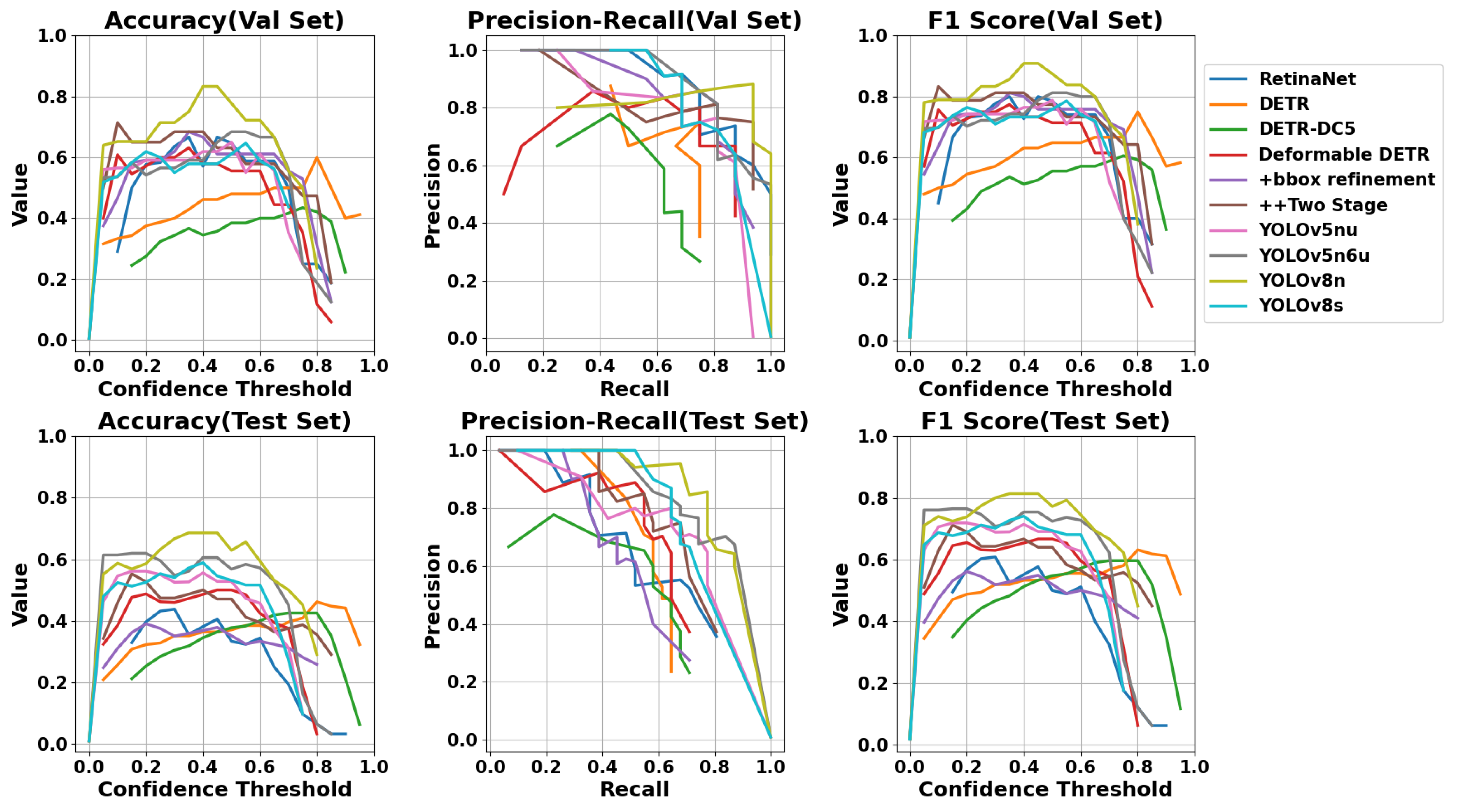
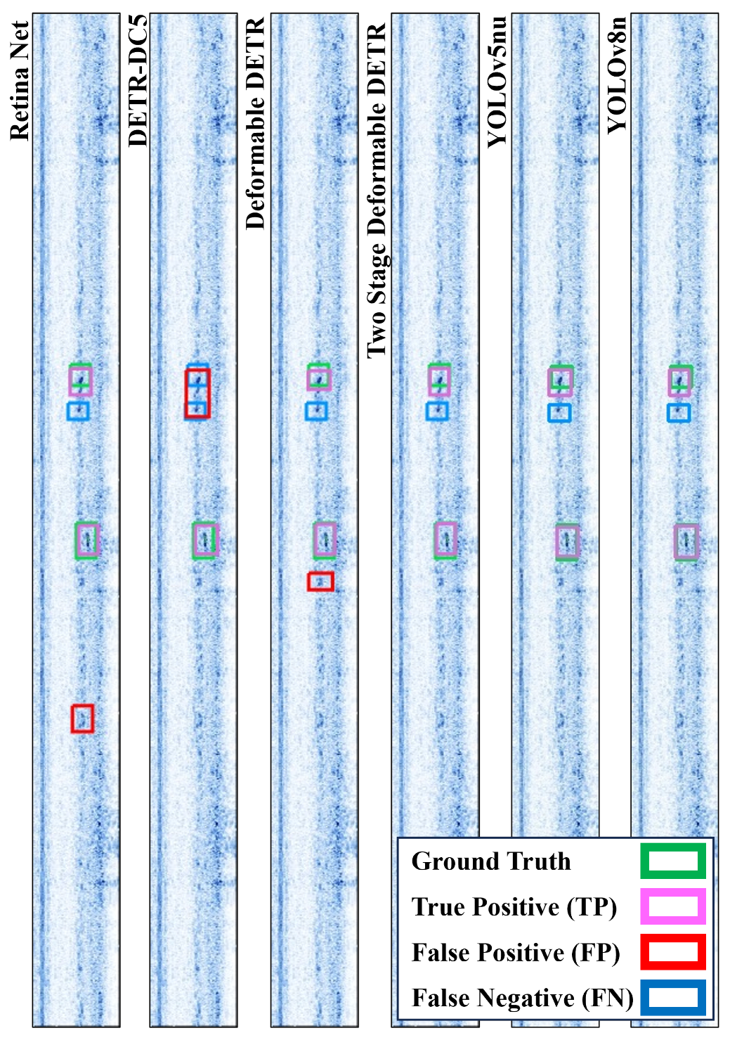
In Figure 14, the accuracy, precision–recall curve, and F1 score on both the validation and test sets for all the fine-tuned models are compared across confidence thresholds ranging from 0 to 1 with a step of 0.05. The four metrics were calculated at each confidence threshold where the model generated at least one correct prediction. In this figure, on the test set, YOLOv8s achieves the highest precision up to the first half of the recall values, while YOLOv8n leads in the second half. DETR-DC5 and DDR50 with the bbox refinement exhibit the lowest precision over recall. YOLOv5n6u outperforms the others up to a confidence threshold of 0.2 in F1 score, with YOLOv8n surpassing the others up to 0.75, and DETR leading for the rest. DETR-DC5 has the lowest F1 score for the first half of the confidence thresholds, while RetinaNet performs poorest for higher thresholds. The interpretations regarding F1 score are consistent with those of accuracy at different thresholds. In the results depicted in by Figure 15, the performance of the six models in detecting LOF flaws from a B-scan image on our test set is demonstrated.

We also investigated the effect of two parameters on the performance of RetinaNet and the DETR-based models. Initially, we repeated the fine-tuning and evaluation procedures by solely modifying the “mean_pixel” from its ImageNet mean_pixel to our train set image mean_pixel. Next, alongside the mean_pixel adjustment, we altered the “test_topK_candidates” (We modified the test_topK_candidates argument of RetinaNet class in detectron2/modeling/meta_arch/retinanet.py) from 1000 to 10 for RetinaNet and “num_queries” (We also set the select_box_nums_for_evaluation parameter of models to 10 to run the training and inference) from 100 to 10 for DETR-based models. In

Table 4. The effect of modification of mean_pixel and topK or num_queries on the performance of the models on the test set. The bold text indicates an improvement relative to the value in Table 3 on the test set.

	mean_pixel				mean_pixel + (topK or num_queries)
Model	ACC	P	R	F1	ACC	P	R	F1
RetinaNet-Res50	−13.75%	−13.83%	−4.76%	−9.98%	−12.61%	+47.02%	−38.10%	−9.12%
DETR-Res50	−16.67%	−5.80%	−16.67%	−12.04%	−45.83%	−33.80%	−38.89%	−36.67%
DETR-DC5-Res50	−21.57%	−14.35%	−17.65%	−16.18%	−32.03%	−26.36%	−23.53%	−24.85%
Deformable DETR-Res50	−21.21%	+1.96%	−23.53%	−15.22%	−53.85%	−37.72%	−47.06%	−43.75%
+bbox refinement	+21.38%	+17.00%	+12.50%	+14.51%	+24.46%	+31.55%	+6.25%	+16.47%
++two-stage	−11.97%	0.00%	−14.29%	−8.05%	−23.10%	−12.82%	−19.05%	−16.21%

, we present the percentage of change relative to the reported values of accuracy, precision, recall, and F1 score in Table 3 on the test set. The results indicate that for DDR50 with box refinement, these modifications led to improvements in all four metrics. Furthermore, the impact of reducing “num_queries” in DETR-based models suggests the need to explore the effects of other parameters, such as “eos_conf”, to enhance the results. This can be investigated in future studies.

In our B-scan images, discriminating an LOF flaw from weld geometry (nonflawed background image) was a challenging task, even for expert operators. This challenge can be addressed by providing more images containing both weld geometry indications and flaws during training. In our images, human operators did not annotate obscure indications of a flaw; however, some of the fine-tuned models detected these types of flaws, resulting in a high count of FPs. This understanding is grounded in the human knowledge and comprehension of the context of the image.

Based on our evaluation of the performance of the fine-tuned models on industrial B-scan images, deploying these models as AI-assisted inspectors can enhance inspection speed and reduce the workload for human UT inspectors in industries utilizing AUT as one of their NDT methods. To address the challenges with industrial usage, one of the main considerations is deploying these deep-learning-based models on the hardware that runs inspection tools. Firstly, these models should be scaled and made more efficient in terms of inference speed and power usage to run on mobile devices, which are the most used in these industries. On the other hand, industries involved in designing NDT inspection tools should be open to providing open-source software that allows different industries to integrate their AI-based models with the acquisition software they use. In our implementation, due to the limitations of the acquisition software, we needed to develop additional software to access B-scan images and prepare them for feeding to the models, which would impact real-time inspection.

5. Conclusions

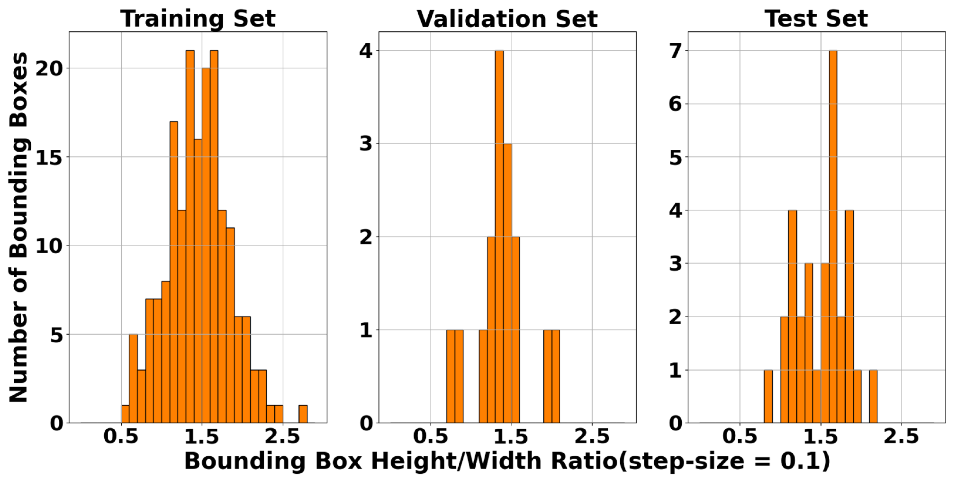
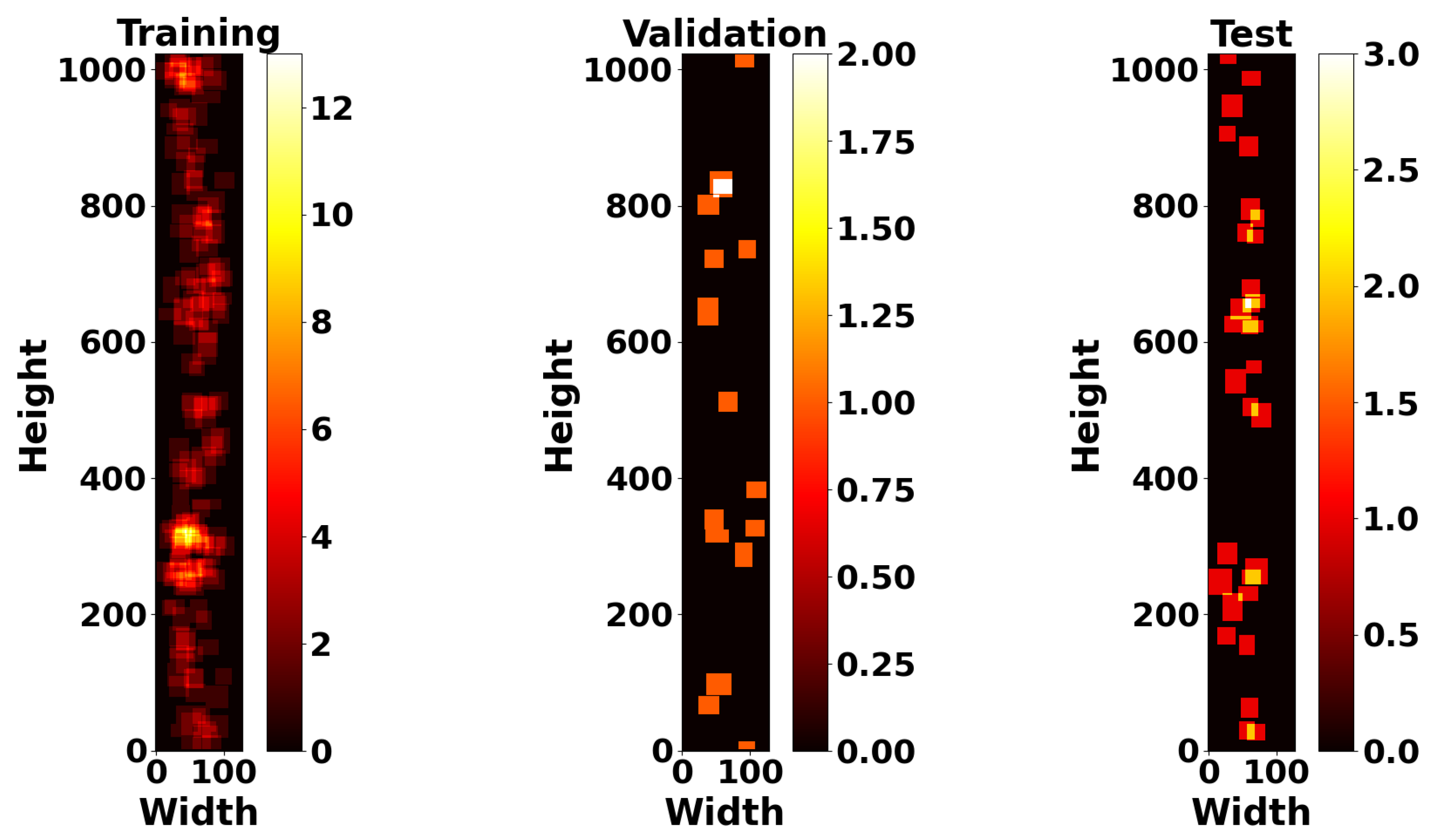
In this paper, we presented a real-world ultrasonic B-scan image dataset, comprising 359 images and 229 annotations for lack of fusion (LOF) flaws. We conducted an extensive analysis of both the image properties and the bounding box properties utilized for annotations. To the best of our knowledge, this is the first time in the literature where industrial B-scan images containing real-world defects were employed for automated weld defect detection using SOTA deep learning models. End-to-end transformer-based object detectors and YOLOv8 were among the fine-tuned models evaluated on our dataset. The selected deep learning models were fine-tuned without any customization in their architectures to establish a baseline benchmark for these models on our dataset. Based on our evaluation, YOLOv8n exhibited superior performance compared to other fine-tuned models in terms of accuracy and F1 score. For the evaluations, we investigated the performance of two types of architectures: CNN-based and transformer-based architectures. According to our results, the CNN architectures with fewer model parameters, without any specific modifications, demonstrate superior performance, specifically compared to a few ten-million-parameter DETR-based models. Among the transformer-based architectures, two-stage Deformable DETR shows the best F1 score, which is 12.53% lower than that of YOLOv8n. Moreover, we demonstrated the effect of different confidence thresholds on the models’ performance using accuracy, precision, recall, and F1 score metrics.

Limitations: While we demonstrated promising applications of deep learning models for industrial B-scan data acquired in the oil and gas industry, it is important to acknowledge the limitations of our work. Our dataset only covers one flaw type, LOF, hindering broader application. Additionally, the limited size of our dataset prevented us from providing a clear view of the inference time required by these models for real-time applications. Though we presented an AI-assisted inspection tool, human evaluation is necessary for missing or incorrect detections. To boost reliability, a human feedback loop may be needed for the model to learn from false positives and negatives. Finally, we did not investigate the effect of the model’s hyperparameters and augmentation techniques on model performance, as we aimed to establish a baseline benchmark for these models. Therefore, we kept default options.

Future Works: For future studies, to enhance the diversity of our dataset, we plan to expand it by acquiring more industrial B-scan images collected during onshore automated girth weld inspections conducted by human UT inspectors. To improve the explainablity of the deep-learning-based models in this field, exploring the application of each layer and component of the models concerning how the B-scan images are processed through them, implementing automated hyperparameter tuning, and investigating the impact of various augmentation techniques on B-scan images, both during training and inference, are crucial for industrial applications. Additionally, studying the applications of new emerging AI-based models, including foundational models, in the field of AUT and analyzing B-scan data in conjunction with other types of ultrasonic data represent interesting ideas for enhancing automated defect detection.