Influence of Tissue Curvature on the Absolute Quantification in Frequency-Domain Diffuse Optical Spectroscopy

Abstract

Accurate estimation of optical properties and hemodynamic parameters is critical for advancing frequency-domain diffuse optical spectroscopy (FD-DOS) techniques in clinical neuroscience. However, conventional FD-DOS models often assume planar air–tissue interfaces, introducing errors in anatomically curved regions such as the forehead or infant heads. This study evaluates the impact of incorporating tissue curvature into forward models for FD-DOS analysis. Using simulations and optical phantoms, we demonstrate that curved models reduce errors in absorption coefficient estimation from 20% to less than 10% in high-curvature scenarios. Within the curvatures tested, even minor curvature mismatches resulted in errors significantly lower than those observed from planar approximations (p < 0.001). In low-curvature regions, curved models yielded errors comparable to planar models (<5% in both cases). When applied to human data, our proposed curved model increased absorption and hemoglobin concentration estimates by 10–15% compared to standard semi-infinite models, closer to physiological expectations. Overall, these results quantitatively demonstrate that accounting for tissue curvature in FD-DOS forward models significantly improves the accuracy of optical property estimation. We propose a numerical framework that achieves this in a fast and reliable manner, advancing FD-DOS as a robust tool for clinical and research applications in anatomically complex regions.

1. Introduction

Over the past three decades, frequency-domain diffuse optical spectroscopy (FD-DOS) has emerged as a potential noninvasive technique for providing absolute quantification of deep tissue [1,2,3]. One FD-DOS approach involves shining an amplitude-modulated light into a region of interest and collecting the backscattered light at multiple distances from the light source. By analyzing the amplitude and phase of the measured signals, it is possible to estimate the absorption and reduced scattering coefficients, denoted as ${\mu }_a$ and ${\mu }_s^{\prime }$, respectively. While scattering offers insights into tissue heterogeneity, absorption coefficients measured at two or more wavelengths are used to determine the concentrations of oxy- and deoxyhemoglobin, which enable the calculation of total hemoglobin concentration and blood oxygen saturation. These hemodynamic quantities hold significant clinical relevance, as total hemoglobin concentration is proportional to blood volume, and blood oxygen saturation reflects the local balance between flow delivery and tissue metabolism [4,5,6,7].

However, the impact of FD-DOS on clinical settings depends on the accuracy of these estimated quantities. Diffuse optical spectroscopy techniques tend to inherently underestimate the optical properties in tissue due to partial volume effects and low-density optical arrays, and current analysis models have limitations in overcoming this challenge. The most common approach to tackle the forward problem involves solving the photon diffusion equation assuming tissue homogeneity and a planar air–tissue interface in the semi-infinite (SI) model [8,9,10]. While this simplification offers an analytically tractable expression for data fitting, it does not capture the complexity of biological tissues. Analytical nonhomogeneous models, such as the two- or three-layered models, attempt to address tissue heterogeneity, particularly in separating extracerebral contributions from brain optical properties [11,12,13,14]. Despite improvements in accuracy, these models still underestimate optical properties [15,16,17,18,19]. In addition, the optimization problem for layered models with FD-DOS is even more ill-posed than the SI case, leading to unstable solutions heavily dependent on the initial guess of their parameters.

The acquisition interface can also influence the inverse problem of parameter estimation. For example, assuming a planar interface has been shown to cause spatial misregistration of functional magnetic resonance imaging and diffuse optical imaging [20]. Additionally, removing data points obtained in poor optode coupling conditions due to interface curvature has effectively reduced image artifacts in diffuse optical tomography [21]. When working with optical data acquired from a curved interface, errors in the blood flow index measured with diffuse correlation spectroscopy (DCS) were estimated to be up to 25% [22]. Furthermore, Monte Carlo simulations in time-domain DOS (TD-DOS) have demonstrated that accounting for the interface geometry results in more accurate assessments of the optical properties [23].

In this work, we quantified the influence of local curvatures at the acquisition interface on the recovery of optical parameters in FD-DOS. Given the numerical instability of implementing analytical models for curved surfaces, we approached this problem by performing numerical simulations of light propagation. The simulations allowed us to build a lookup table for the forward problem, which was then utilized during the solution of the inverse problem to estimate tissue optical properties. We initially validated our approach using planar phantom surfaces and compared the results with those obtained using the standard SI approach in curved phantoms and head simulations. Subsequently, we evaluated the effect of curvature on estimations of optical properties using human data.

2. Materials and Methods

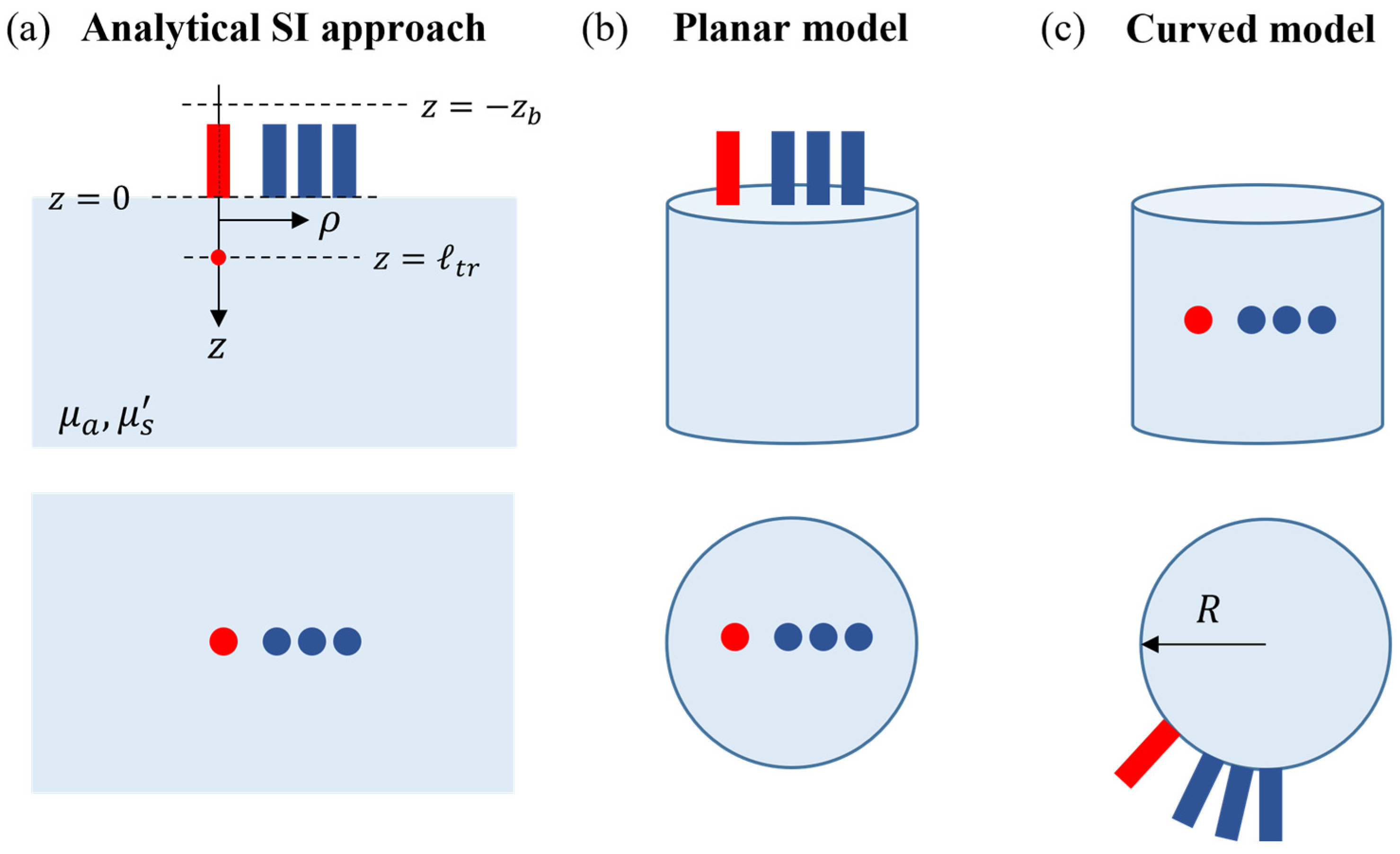
2.1. Forward Models for Parameter Estimation

Recovery of optical properties from FD-DOS data can be mathematically formulated as an optimization problem:

$${\mu }^{\star }=arg min F\left({\mu }^{\prime }\right),$$

(1)

where ${\mu }^{\prime }\in {\mathbb{R}}^D$ is a D-dimensional vector containing the optical properties relevant to the model, ${\mu }^{\star }$ denotes the optimal solution, and F represents an error function that minimizes the difference between the measured quantities and those predicted by a model. A commonly used error function for this problem is the squared error function [15]:

$$F=F_A+F_{\theta }$$

(2)

where

$$\begin{array}{c}{F}_A={\displaystyle \sum _{i=2}^N}{\left(log \left({\displaystyle \frac{A^{model}\left({\rho }_i\right)}{A^{model}\left({\rho }_1\right)}}\right)-log \left({\displaystyle \frac{A^{data}\left({\rho }_i\right)}{A^{data}\left({\rho }_1\right)}}\right) \right)}^2,\\ F_{\theta }={\displaystyle \sum _{i=2}^N}{\left(\left({\theta }^{model}\left({\rho }_i\right)-{\theta }^{model}\left({\rho }_1\right)\right)-\left({\theta }^{data}\left({\rho }_i\right)-{\theta }^{data}\left({\rho }_1\right)\right)\right)}^2.\end{array}$$

Here, ${\rho }_i$ represents the distance of the i-th source–detector separation (SDS), $N$ is the total number of SDSs, and $A\left({\rho }_i\right)$ and $\theta \left({\rho }_i\right)$ are the fluence amplitude and phase shift measured at ${\rho }_i$, respectively. The superscripts “model” and “data” denote the quantities predicted by the forward model and the measured quantities, respectively.

To solve this optimization problem analytically with respect to the optical parameters, we utilized the interior-point algorithm implemented by the “fmincon” function in MATLAB 20201a (The MathWorks Inc., Natick, MA, USA). In our study, this problem was solved for three different forward models (Figure 1). For simplicity, all models were assumed to be homogeneous, so we could investigate the effects of curvature without adding any cofactors to the analysis. This assumption also reduces the dimensionality of the problem to only two parameters (${\mu }_a$ and ${\mu }_s^{\prime }$).

2.1.1. Analytical Semi-Infinite Model

The first model we tested was the analytical solution of the photon diffusion equation to the semi-infinite (SI) geometry with the extrapolated boundary condition [10,24,25]. The SI approach is widely used in the literature due to its simplicity and low computational cost. It assumes the biological tissue as a homogeneous medium, infinite in the x- and y-directions, with a single air–tissue boundary in the z-direction (Figure 1a). For FD-DOS, the photon fluence, $\varphi$, at the interface ($z=0$) is given by the following:

$$\varphi \left(\overrightarrow{r},\omega \right)={\displaystyle \frac{v}{4\pi D}}\left[{\displaystyle \frac{e^{-k{r}_1}}{r_1}}-{\displaystyle \frac{e^{-k{r}_b}}{r_b}}\right],$$

(3)

where $v$ is the speed of light inside the tissue, $D=v$/$3\left({\mu }_a+{\mu }_s^{\prime }\right)$, $r_1=\sqrt{{\left(z-{\mathcal{l}}_{tr}\right)}^2+{\rho }^2}$, $k^2=\left(v{\mu }_a+i\omega \right)$/$D$, $\omega =2\pi f$ ($f$ is the source modulation frequency), and $r_b=\sqrt{{\left(z+2z_b+{\mathcal{l}}_{tr}\right)}^2+{\rho }^2}$. Here, ${\mathcal{l}}_{tr}={\left({\mu }_a+{\mu }_s^{\prime }\right)}^{-1}$ is the depth where the point-like source is assumed, $\rho$ is the planar distance between the source and the detector along the interface, and $z_b=2{\mathcal{l}}_{tr}\left(1+R_{eff}\right)$/$3\left(1-R_{eff}\right)$ is the distance outside the interface where $\varphi$ is assumed to be zero, where $R_{eff}$ is the effective Fresnel reflection coefficient (see Figure 1 for the geometrical representation of these quantities).

2.1.2. Numerical Models

In addition to the SI approach, we used the finite-element method (FEM) to solve the forward problem and predict the expected amplitude and phase of FD-DOS data for two specific geometries. The simulations were performed using the open-source software NIRFASTer 9.1 [26,27] with a node size of 0.065 cm, which provided final meshes containing 610,001 nodes. All data were generated on a desktop computer with an AMD Ryzen 7 2700 eight-core processor (3.2 GHz), 32 GB of RAM, a 240 GB SSD, and Windows 10 Pro 64-bit.

The first geometry consisted of a homogeneous cylinder (radius and height of 9 cm) with the source and detectors positioned at the center of the top planar surface (Figure 1b). This planar surface aimed to confirm the reliability of the numerical solution compared to the analytical SI approach.

The second geometry used the same cylinder as before, but the sources and detectors were positioned on a plane parallel to the cylinder basis (Figure 1c). With this approach, the side of the cylinder can mimic tissue curvatures, since the cylinder radius, R, determines the interface curvature, $\kappa$ (i.e., $\kappa =1/R$). In this work, we simulated two curvatures with radii of 9 and 7 cm (corresponding to $\kappa =0.111 \mathrm{c}{\mathrm{m}}^{-1}$ and $0.143 \mathrm{c}{\mathrm{m}}^{-1}$, respectively), which we refer to as curved model 1 and curved model 2, respectively. These values were chosen due to their proximity to actual forehead curvature measurements in adults.

For each geometry, we varied ${\mu }_a$ from 0.05 to 0.30 in steps of 0.005 $\mathrm{c}{\mathrm{m}}^{-1}$, and ${\mu }_s^{\prime }$ from 5 to 15 in steps of 0.1 $\mathrm{c}{\mathrm{m}}^{-1}$. The amplitude and phase for each cross-combination were stored as a lookup table that was used as an alternative approach for solving the optimization problem (Equation (1)) to estimate the absolute optical properties from the FD-DOS data.

2.2. Validation Datasets

We tested the forward models in three distinct scenarios: conducting numerical simulations in geometries mimicking phantoms, using experimental data obtained from homogeneous optical phantoms with known optical properties, and performing numerical simulations on an adult human head.

2.2.1. Numerical Simulations in Mimicking Phantoms

The first step was to compare the models involved by performing numerical simulations in media that mimicked optical phantoms. For this, we created two meshes consisting of homogeneous cylinders with different curvatures. For the cylinder with low curvature (11 cm radius, curvature $\kappa =0.091 \mathrm{c}{\mathrm{m}}^{-1}$; mesh node size of 0.9 cm, comprising 645,643 nodes), we placed one source and one detector on both the curved and planar sides. For the cylinder with high curvature (5 cm radius, curvature $\kappa =0.200 \mathrm{c}{\mathrm{m}}^{-1}$; mesh node size of 0.9 cm with 148,836 nodes), we positioned the source and detector only on the curved side. These simulations were conducted within the same parameter ranges described previously (Section 2.1.2).

We added random amplitude and phase noise to each simulation independently. For phase, the noise was based on a Gaussian model with a zero mean and a standard deviation of 0.1 degrees. For amplitude, noise was incorporated such that the signal-to-noise ratio of the resulting curve reached 100, similar to previous research [28]. Then, we fitted the resulting simulated data using the methods outlined in Section 2.1 for each combination of optical properties and curvature.

2.2.2. Phantom Measurements

We also compared the performance of each algorithm with experimental data obtained from two commercial optical phantoms (ISS, Inc., Champaign, IL, USA). The phantoms consist of blocks primarily made of silicone and have known optical properties, with absorption coefficients varying between 0.10 and 0.11 cm⁻¹ and scattering coefficients varying between 9 and 11 cm⁻¹ for 690 and 850 nm. Each block comprised three different interfaces for data acquisition: the planar top of the block and two curved sides with the same radius as the simulated phantoms (i.e., 5 and 11 cm). We collected data at all interfaces in both phantoms for 2 min and fitted each data point to the different models depicted in Figure 1 separately.

All experiments were performed with a commercial FD-DOS system (Imagent, ISS, Inc., Champaign, IL, USA). We used four sources of two laser diodes with distinct wavelengths (690 and 847 nm) modulated at 110 MHz and one photomultiplier tube as a detector. The optical probe contained four source–detector separations, with distances of 1.5, 2.0, 2.5, and 3.0 cm. The temporal resolution of the data acquisition was 18.4 Hz. Before every measurement, we calibrated the device using standard procedures to ensure the accuracy of the measured amplitude and phase [1,29,30].

2.2.3. Numerical Simulations on a Realistic Head

To examine the influence of curvature on recovering the absolute optical properties in head geometries, we created a head mesh using an open-source library (brain2mesh, with a Delaunay sphere radius of 0.11 cm, radius-to-edge ratio of 1.24, and maximum element volume of 4 cubic voxels) [31] and then used this mesh as input into NIRFASTer. We performed simulations at two locations on the parietal lobe of the head with distinct curvatures: one region with high curvature (7 cm radius, corresponding to $\kappa =0.143 \mathrm{c}{\mathrm{m}}^{-1}$) and another region that was relatively flat (radius = 20 cm, $\kappa =0.050 \mathrm{c}{\mathrm{m}}^{-1}$), which we refer to as high- and low-curvature datasets, respectively. (Note, the curvature was estimated by computing the radius of the circumcenter that passes through the boundary vertices located between the source and the farthest detector). At each location, we simulated a probe with four SDSs (1.5, 2.0, 2.5, and 3.0 cm). Simulations were performed varying ${\mu }_a$ from $0.1$ to $0.25$ $\mathrm{c}{\mathrm{m}}^{-1}$ in steps of $0.05 \mathrm{c}{\mathrm{m}}^{-1}$, and ${\mu }_s^{\prime }$ from $6$ to $12 \mathrm{c}{\mathrm{m}}^{-1}$ in steps of $2 \mathrm{c}{\mathrm{m}}^{-1}$, always assuming a homogeneous medium, to which noise was added using the same noise model described in Section 2.2.1.

For all datasets, the performance of each fitting model was assessed by calculating the median of the absolute percentage error (MAPE), defined as the median of the quantity across all time points:

$$\left|{\displaystyle \frac{y_{pred}-y_{truth}}{y_{truth}}}\right|\times 100\%$$

(4)

In the equation above, y represents the quantities under investigation (i.e., optical properties or their derived physiological quantities), and the subscripts “pred” and “truth” represent the values of these quantities estimated by the fitting procedure and their ground truth, respectively.

In all cases, we report the MAPE and the 95% confidence interval in the results below. We used a two-sided Wilcoxon rank sum test to assess differences between paired MAPE distributions, reporting statistical significance using p-values. However, given the large number of simulated data points, which can artificially lower p-values, we also quantified the magnitude of differences between approaches (i.e., its effect size) by comparing the frequency histograms using the scaled robust estimator for Cohen’s d to account for non-parametric distributions [32].

2.3. Human Brain Dataset

To evaluate the performance of all models in actual human data, we collected FD-DOS data obtained from 152 healthy participants [33], whose main demographic information is presented in

Table 1. Number of participants and mean age of all participants recruited for this study, separated by cofactors (sex, skin color). The values in parentheses represent the standard deviation across the sample distribution.

		Sex		Skin Color
	Total	Men	Women	White	Non-White (NW)
Participants	152	55	97	99	53
Age [years]	39 (17)	39 (18)	38 (17)	37 (17)	41 (17)

. All participants were instructed to sit in a chair, stay relaxed, and not move. The optical probe comprised one detector and four sources located 1.5, 2.0, 2.5, and 3.0 cm away from the detector, and it was placed on seven regions of interest (ROIs) around the prefrontal cortex using adhesive tape (see Supplementary Figure S1 for the measured head locations). For every participant, we collected a two-minute data segment at each ROI. All experimental procedures were reviewed and approved by the local ethics committee at the University of Campinas, where the experiments were carried out.

For data analysis, we discarded (1) time points where amplitude did not decrease, or phase did not increase, with an increase in SDS, and (2) data points whose ${{\mu }_s}^{\prime }$ estimate at 690 nm was higher than 847 nm. Both conditions do not match the expected behavior for light propagation in tissue and likely result from experimental errors due to poor probe contact. From the estimation of the optical properties, we used the modified Beer–Lambert law to calculate oxy- and deoxyhemoglobin concentrations ($\left[HbO\right]$ and $\left[HbR\right]$, respectively) directly from ${\mu }_a$. As we acquired data at two wavelengths, we assumed a water fraction of 75% to obtain chromophore concentrations with more reliability. This value falls between the expected water fractions of gray and white matter [34] and is close to those used in prior studies [35,36]. From the hemoglobin concentration, we calculated the total hemoglobin concentration, [HbT] = [HbO] + [HbR] and the cerebral oxygen saturation, StO₂ = [HbO]/[HbT].

3. Results

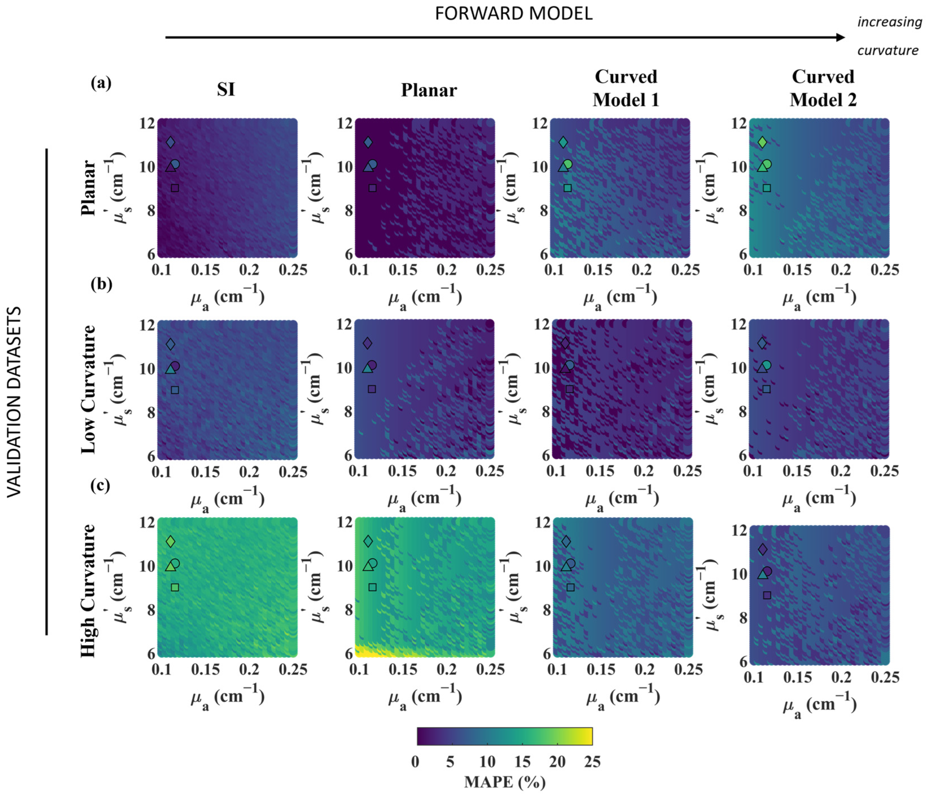
3.1. Effect of Curvature on Phantoms

Figure 2 presents the absolute percentage errors (MAPEs) for the recovered absorption coefficients of the simulated phantoms when the probe was positioned in both planar and curved interfaces, analyzed with the different forward models over the range of optical properties tested.

When the source and detector were positioned on a planar surface (Figure 2a), the errors were consistently low (<10%), regardless of the forward model used for fitting. The lowest MAPEs were observed for planar models, i.e., the analytical semi-infinite (SI) model and numerical model with the probe on the planar surface. The average MAPE (95th confidence interval) was 2.8 (0.5, 4.6) % for the SI model and 0.2 (0.0, 3.2) % for the planar numerical simulation across all properties simulated. Fitting the data obtained in the planar acquisition interface with curved models resulted in slightly higher MAPEs of 4.5 (2.2, 8.0) % and 6.5 (4.3, 9.5) % when the curvature radii of the cylinder in the forward model were set at 9 and 7 cm, respectively. Despite the small errors overall, the introduction of a curved model to fit a perfectly planar situation introduced a significantly larger error when compared to planar models (p < 0.001, Cohen’s d = 1.7).

On the other end, curved models significantly outperformed planar models when the optical probe was positioned on highly curved surfaces (Figure 2c). The lowest error rate was obtained when the mismatch between the curvature of the measurement interface and the curvature of the forward model was minimal (i.e., 7 cm radius; MAPE: 5.6 (2.8, 8.7) %). However, even when the curvature of the model slightly differed from the actual interface curvature, the errors were still comparable (9 cm radius, MAPE: 6.8 (4.2, 10.3) %) and were not significantly different from the case of a perfect match (p < 0.001, d = 0.8). Conversely, planar models yielded significantly higher errors when used to fit such highly curved interfaces (p < 0.001, d = 3.9), with average MAPEs almost double of those found by curved models (13.3 (10.3, 16) % for the SI model and 12.3 (9.1, 25) % for the planar model).

For the intermediate case of an existing-but-less-pronounced curvature (Figure 2b), both curved and planar models yielded comparable errors (p < 0.001, d = 0.6). Similar to the previous case, the curved model that matched the actual interface curvature resulted in the smallest error (MAPE = 2.2 (0.0, 5.3) %). Using a curved model with a small discrepancy in curvature introduced an additional average error of approximately 1% compared to the optimal scenario (MAPE = 3.8 (0.0, 7.7) %), but this condition was still more favorable than assuming no curvature at all, which resulted in an average additional error of 2.2%. For the low-curvature interface, the use of planar models resulted in MAPEs of 4.8 (2.5, 6.8) % and 3.6 (0.0, 9.1) % for the SI model and planar simulation, respectively.

The experimental data collected from the phantoms were positioned as markers in Figure 2 for direct comparison with the simulations. Overall, the errors obtained for the optical phantoms were slightly higher than those calculated for the simulated phantoms due to the presence of actual measurement noise. Despite the larger errors, the experimental data points followed the same trends observed in the phantom simulations. When fitting planar interfaces, curved models yielded average MAPEs of 13.6 (9.1, 19.5) % across all wavelengths and phantoms, substantially higher than the 3.8 (0.0, 7.4) % obtained with planar models for this condition. As the measurement surface exhibited a low-but-nonzero curvature (11 cm radius), the MAPEs obtained with planar models slightly increased to 4.5 (1.8, 9.1) %, while the errors associated with curved models decreased by half, to an average of 6.2 (0.0, 10.6) %. The highest errors occurred when using planar models to fit data obtained in highly curved interfaces, resulting in average MAPEs of 11.5 (7.1, 18.2) % (planar numerical) and 15.4 (12.7, 18.9) % (analytical SI). Conversely, curved models achieved MAPEs ranging from 3% to 7% in this situation.

Lastly, when comparing the errors obtained by the numerical planar model and the analytical SI model across all situations, we did not observe significant differences (p < 0.001, d = 0.2). Given that MAPE distributions are particularly skewed due to their bounded nature at zero, we further assessed the stability of these two approaches using their 95th percentile. In all cases, the 95th percentile was around 5% (Supplementary Table S1), reinforcing that our approach based on numerical models was as robust as the analytical approach to fit FD-DOS data with the same condition. Given the similarity in performance between these planar models, we focused the remaining comparisons of the curved models on the SI model only.

3.2. Model Validation in Head Simulations

Figure 3 shows the performance of different models (measured by the MAPE) as a function of the simulated optical properties for the two curvature values examined. Specifically, we report the MAPE of the recovered absorption coefficient (${\mu }_a^{fit}$) relative to the simulated absorption coefficient (${\mu }_a^{sim}$) for four reduced scattering coefficients in the forward model. In regions of the head with low curvature (Figure 3a), the behavior of the curved models closely paralleled that of the SI model, with no significant differences (p = 0.38, d = 0.3). The average MAPE across all tested values of ${\mu }_a$ and ${\mu }_s^{\prime }$ was 5.0 (0.0, 18.0) % when using the curved model that closely matched the local head curvature (9 cm radius), and 6.1 (0.8, 19.2) % for the SI model. The stability of the models was also similar: the 95th percentile range was around 4.1% for the SI model on average, close to the 5.5% measured for the curved models.

In regions of the head with high curvature (Figure 3b), the planar approach yielded significantly higher errors than the curved models (p < 0.001, d = 1.1). The average MAPE for recovering ${\mu }_a$ across all simulations was 9.7 (2.5, 22.1) % for the SI model, which is larger than the 5.0 (0.0, 15.0) % obtained for the curved model that matched the head curvature (7 cm radius). Interestingly, using a curved model with a different curvature (9 cm radius) yielded a similar MAPE of 5.0 (0.0, 10.0) % (p = 0.11, d = 0.4). The 95th percentile range obtained for the curved and SI models was 3.3% and 2.8%, respectively.

When analyzed as a function of the optical properties, the errors tended to increase with higher values of ${\mu }_a$ and decrease with higher values of ${\mu }_s^{\prime }$ for all models. A direct comparison between the models showed that the analytical SI approach consistently yielded higher errors compared to the curved models across all ranges of optical properties tested. The impact of curvature on the estimation of optical properties was particularly high in regions with high ${\mu }_a$ and low ${\mu }_s^{\prime }$ values, wherein the planar models consistently yielded higher MAPE values.

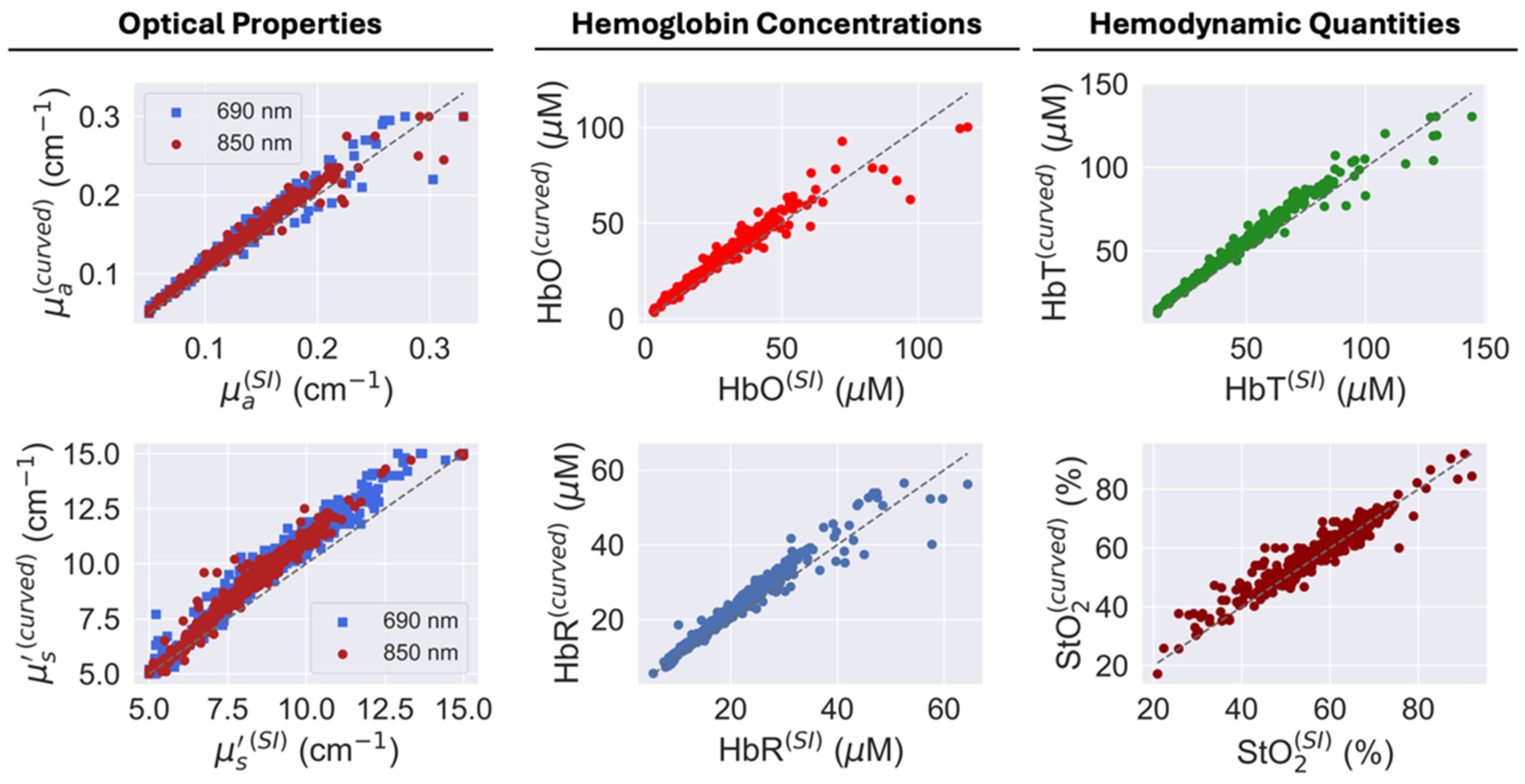
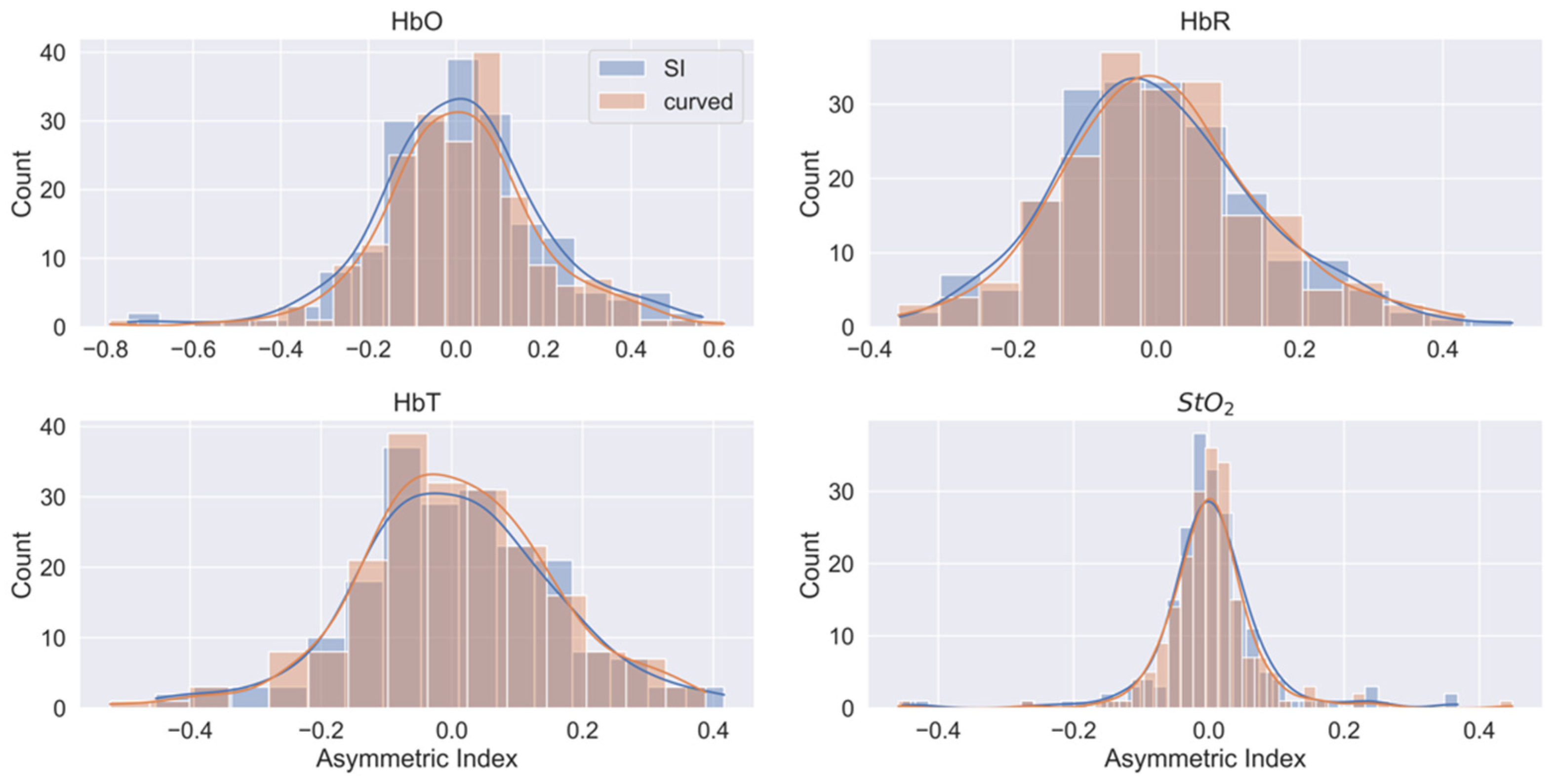
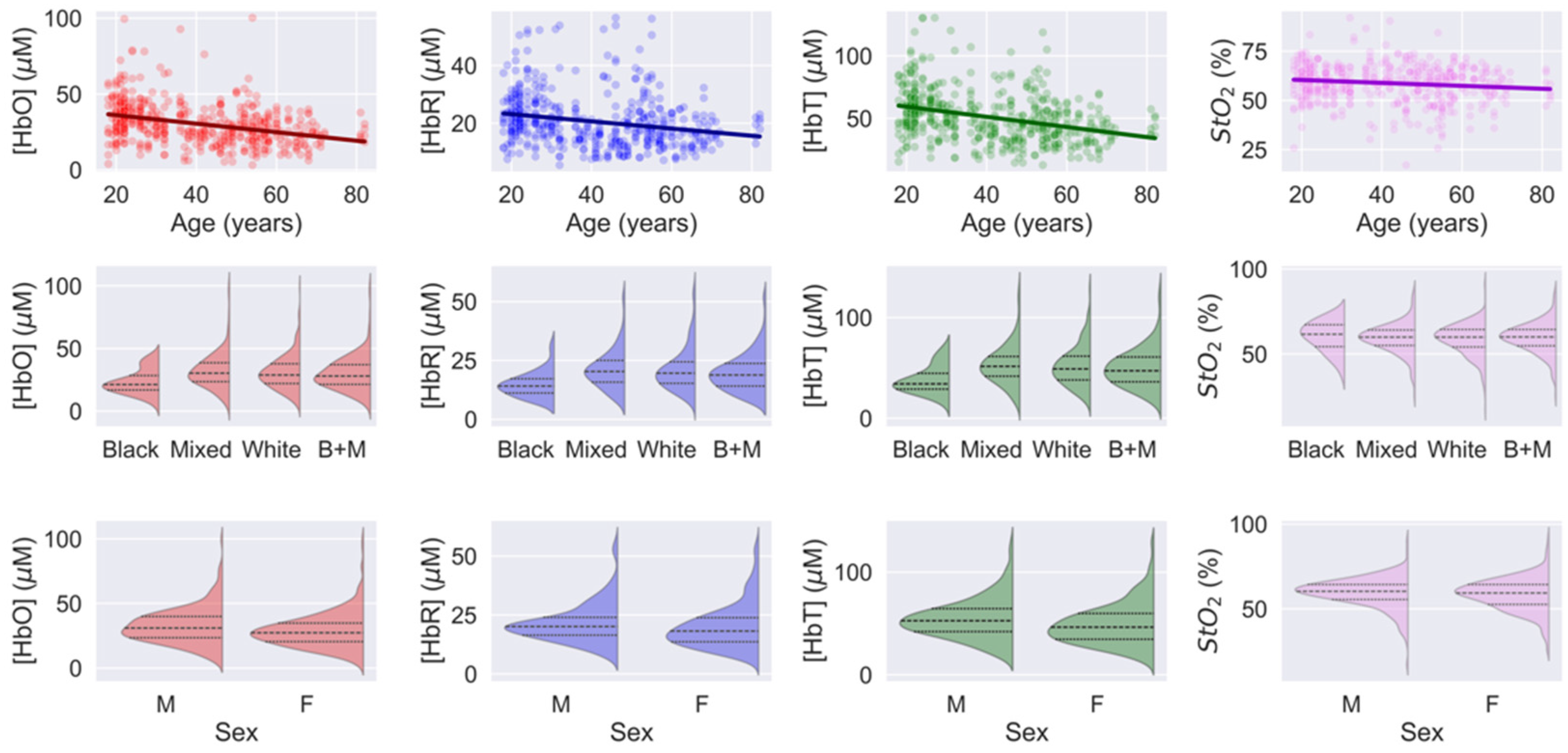
3.3. Human Head Measurements

When applied to actual human data, we observed that using the cylinder with high curvature (7 cm radius) as the forward model increased the absolute quantification of the optical properties by approximately 10% compared to the SI model while maintaining the same level of variability (

Table 2. Mean and 95% confidence interval of the optical properties and physiological parameters estimated for the FD-DOS data on the forehead when using the standard semi-infinite (SI) model and the curved model (7 cm radius).

Comparison of the Estimated Parameters in FD-DOS Using Different Models
Optical properties
	690 nm		850 nm
	absorption (cm−1)	scattering (cm−1)	absorption (cm−1)	scattering (cm−1)
Curved	0.120 (0.116; 0.124)	9.91 (9.72; 10.1)	0.134 (0.130; 0.138)	8.77 (8.61; 8.93)
SI	0.110 (0.107; 0.114)	8.92 (8.75; 9.08)	0.123 (0.119; 0.127)	8.00 (7.87; 8.14)
Physiological parameters
	[HbO] ($\mathsf{\mu }$molar)	[HbR] ($\mathsf{\mu }$molar)	[HbT] ($\mathsf{\mu }$molar)	StO2 (%)
Curved	30.5 (29.3; 31.6)	20.7 (19.9; 21.4)	51.1 (49.4; 52.8)	58.9 (58.1; 59.7)
SI	27.1 (25.9; 28.3)	19.0 (18.3; 19.7)	46.1 (44.4; 47.8)	57.6 (56.8; 58.4)

, Figure 4). Combining both wavelengths, the mean (95% CI) increase in the absorption and scattering coefficients across all participants were, respectively, 9.5 (9.2; 9.8) % and 10.1 (9.7; 10.4) %. The increase in absorption also extended to the estimations of hemoglobin concentrations: 15.4 (14.5; 16.2) % for HbO, 9.1 (8.5; 9.8) % for HbR, and 12.2 (11.8; 12.7) % for HbT. Across all hemodynamic properties, StO₂ exhibited the lowest sensitivity to curvature, showing a modest increase of 2.7 (2.2; 3.3) %.

When comparing the different measurement locations on the head, the curved model consistently increased the estimated quantities in all areas by approximately the same amount, with no significant differences observed between measurements taken more laterally on the forehead or closer to the center of the head.

The increase in absolute quantification was consistent across the entire sample, thus not affecting the overall distribution of the physiological parameters across the different demographic factors investigated. The asymmetry index (calculated as (left − right)/(left + right) of the hemodynamic parameters measured in symmetric regions) remained the same for both the curved and SI models, with the variability in the curved model being slightly smaller (Figure 5).

This consistency was also observed when analyzing the distribution of each quantity as a function of participant demographics, as shown in Figure 6 for the curved model. We found no significant differences in distributions based on sex (male vs. female) or skin color, even when analyzed separately or combining black and mixed races as a “non-white” category. (Note, we combined these two categories due to their lower number of samples compared to “white”.) The relationship between hemodynamic quantities and age showed a consistent decrease in chromophore concentration with increasing age for all hemoglobin contrasts. Linear regression analysis indicated that HbO and HbT were more sensitive to age, while oxygen saturation showed only a weak correlation with age (

Table 3. Slope and intercept of the linear regression analysis for all hemodynamic parameters as a function of participants’ age.

	Slope	Intercept	Pearson Correlation Coefficient
HbO [$\mathsf{\mu }$M]	−0.28 (0.03)	42 (5)	−0.35 (p < 10−5)
HbR [$\mathsf{\mu }$M]	−0.13 (0.02)	26 (1)	−0.23 (p < 10−5)
HbT [$\mathsf{\mu }$M]	−0.41 (0.05)	67 (2)	−0.34 (p < 10−5)
StO2 [%]	−0.08 (0.02)	62 (1)	−0.14 (p = 0.02)

). In all these cases, the slopes obtained with the SI model were close to those obtained with the curved model, indicating that despite increasing the absolute values, the curved model maintained consistency in their dependencies with participants’ demographics.

4. Discussion

The ability to accurately determine absolute values of tissue optical properties is key in translating diffuse optics to clinical settings, as these values provide more specific and interpretable insights compared to relative measurements. Absolute quantification enables comparisons across individuals, cohorts, and studies, enhancing the generalizability of research findings and offering clinical potential as direct biomarkers of brain physiology without the need to induce changes [5,37,38,39]. This work aimed to quantitatively assess how accounting for curvature at tissue interfaces impacts the estimation of absolute optical properties and their derived hemodynamic quantities as measured by FD-DOS.

Most previous FD-DOS investigations have relied on the simplifying assumption of flat tissue surfaces, ignoring curvature. While researchers often place optical probes in low-curvature regions to minimize these effects, certain scenarios—such as measurements on infant heads or inherently curved regions like the occipital lobe or specific upper limb muscles—require dealing with curved tissues. Understanding the implications of curvature on FD-DOS results and developing strategies to account for its effects can significantly improve the accuracy of optical property estimation.

At first glance, one might assume that curvature primarily affects the source–detector separation, a critical factor in diffuse optical techniques. However, even in regions with relatively high curvature, the change in SDS due to curvature is minimal; for example, a curvature of 0.2 cm⁻¹ changes SDS by only 3% at a 4 cm distance. This small change cannot account for the 10–20% errors observed in this study. Instead, the primary challenge posed by curved interfaces lies in the modified symmetry and boundary conditions for the photon diffusion model.

To address the computational challenges posed by photon diffusion in curved geometries, we employed lookup tables to solve the inverse problem and estimate optical properties by minimizing the difference between predicted and measured amplitude and phase data using multi-distance FD-DOS. When compared to analytical approaches, this strategy allows for real-time estimation by reducing the computational time once generated, albeit at the cost of memory requirements. To map a tractable search space, we used a reduced four-dimensional parameter space encompassing $\{{\mu }_a,{\mu }_s^{\prime },SDS,R\}$, with SDS values fixed by the experimental setup. The chosen step sizes for ${\mu }_a$ and ${\mu }_s^{\prime }$ provided sufficient resolution for our research objectives considering the typical noise levels observed in FD-DOS data, yielding resolutions of 1.5 μM for [HbO], 0.9 μM for [HbR], 1.8 μM for [HbT], and approximately 0.4% for StO₂. The similar performance of the planar model and the analytical $SI$ model validates the accuracy of our lookup table methodology. If a higher resolution is needed, interpolation of simulated values [40] or machine learning approaches could be explored, though the latter may not always converge to optimal solutions.

Our results demonstrate that incorporating curvature into forward models significantly reduces errors in FD-DOS measurements performed on realistic interfaces. Curved models outperformed planar models in nearly all scenarios, with the exception of perfectly flat surfaces, such as those used in optical phantom calibration. In such cases, curved models introduced errors of approximately 11 (5)%. The increased errors of curved models in near-planar conditions are likely due to overfitting, as the introduction of unnecessary geometric corrections increases the degrees of freedom of the problem. In addition, the change in boundary conditions introduced by the curved setups in the numerical forward model can lead to discretization errors or mesh irregularities that may propagate to larger errors in the estimation of the optical properties. Nevertheless, semi-planar scenarios are not representative of real-world conditions, as all tissue surfaces have some degree of curvature.

In scenarios with even slight curvature, our validation experiments showed that curved models did not harm the estimation of the optical properties. Both optical phantoms and head simulations indicated that fitting data from low-curvature regions with curved models produced results comparable to those obtained with planar models, with errors ranging from 2 to 13%, depending on the optical properties of the medium. However, as curvature increased curved models consistently outperformed planar models, reducing errors from up to 20% to less than 10% in most cases. This finding is consistent with earlier studies reporting 15–20% inaccuracies in ${\mu }_a$ estimation due to curvature mismatches [23].

In our validation analysis, we constrained curvature to two values within specific limits related to the average curvature of the adult head, as our goal was to explore the effects of incorporating curvature and not quantifying the effect of specific curvature values in FD-DOS. By making it clear that curvature is relevant, future applications can measure local curvature using digital tracking systems (e.g., digitizers) or by computing the radius of the circumcenter that passes through the boundary vertices located between the source and the farthest detector. When curvature cannot be determined, our data indicate that errors associated with slight deviations in curvature remain within 5 (2)% (Figure 2 and Supplementary Table S1), which is smaller than the errors introduced by planar approximations.

When applied to human data, incorporating curvature increased the absolute quantification of optical properties by an average of 10 (5)% compared to the SI model. This increase translated into a 15 (10)% increase in [HbO], a 9 (8)% increase in [HbR], and a 12 (5)% increase in [HbT] (Table 2). StO₂ was the least affected, showing only a 2% increase, as changes in [HbT] and [HbO] compensate for each other. Despite these increases, the absolute values remained lower than those reported by TD-DOS [35], likely due to our homogeneous assumption. Here, we restricted our analysis to homogeneous models only to isolate the impact of curvature without introducing additional confounding factors. While this simplification limits the physiological interpretation of the human results, it provides a controlled framework to quantify curvature-specific errors. Incorporating layered models could further increase the values and improve accuracy [15,16,17,18,19,41,42,43,44], but this requires additional source–detector separations to constrain the increased parameter space introduced by the extra model layers [15,17], which our probe configuration did not support. Since curvature and tissue heterogeneity represent independent sources of error, future investigations integrating both factors and using a probe with greater source–detector separations will likely achieve even higher accuracy than layered models alone. Although the lookup table framework described in this work could be extended to layered, curved media, generating such a table would be considerably more computationally intensive. Recent advances in machine learning and adaptive interpolation could reduce computational costs by approximating solutions for layered, curved geometries. Future work should explore hybrid frameworks by combining these techniques with our curvature framework, enabling simultaneous correction for tissue heterogeneity and interface curvature.

Importantly, the introduction of curvature did not alter the distribution of hemodynamic parameters across demographic factors. For example, the age-related decline in hemoglobin concentrations was consistent across models and aligned with findings previously reported [35,45,46]. Together, these findings strengthen confidence in longitudinal studies and reinforce the use of absolute values from FD-DOS as potential biomarkers for clinical applications.

It is also worth noting that the inaccuracies in optical properties have broader implications for other techniques, such as continuous-wave diffuse correlation spectroscopy (DCS), where blood flow index (BFI) estimations depend on optical properties often obtained with FD-DOS. Although BFI estimations were not directly sensitive to curvature in phantom simulations, errors in the optical properties due to curvature in FD-DOS resulted in BFI errors of approximately 10% (Appendix A). This further highlights the importance of addressing accuracy in optical property estimation, as it can indirectly affect other derived parameters.

Finally, while using curved models in the forward problem proved effective, this is not the only way to address curvature in FD-DOS. An alternative approach involves calibrating the FD-DOS device on an optical phantom with known optical properties and a curved surface. In fact, when the curvature of the calibration surface matched the measured surface, MAPEs decreased to an average (standard deviation) of 3 (1)% (see Supplementary Table S2). However, this approach requires precise curvature matching between the calibration phantom and the measured tissue. In cases where there was a mismatch, MAPEs increased to approximately 10 (1)%, slightly higher than those obtained with our proposed curved model. This suggests that integrating curvature into forward models offers a robust and scalable solution, significantly improving FD-DOS reliability for both research and clinical applications.

5. Conclusions

In conclusion, this study demonstrates that incorporating tissue curvature into FD-DOS forward models substantially enhances the accuracy of optical properties and hemodynamic parameter estimation. Curved models consistently outperformed planar approaches, reducing errors from up to 20% to less than 10% in high-curvature scenarios while introducing minimal errors (~5%) into low-curvature regions. Across curvature values tested, we found that curved models minimized errors compared to planar approximations, even when there were mismatches in curvature values, which supports their use even when precise curvature measurements are not readily available and offers practical flexibility for clinical applications where precise curvature measurements are challenging.

Applied to human data, curved models increased absorption and hemoglobin concentration estimates by ~10–15%, bringing them closer to physiological expectations while maintaining consistency in demographic trends. This reinforces FD-DOS as a robust tool for longitudinal and population-level studies, and future work should integrate curvature and layered models to address tissue heterogeneity and irregular geometries simultaneously. However, the advances presented here improve FD-DOS reliability toward broader clinical adoption, particularly in scenarios where anatomical curvature is unavoidable.

References

1. Fantini, S.; Sassaroli, A. Frequency-Domain Techniques for Cerebral and Functional Near-Infrared Spectroscopy. Front. Neurosci. 2020, 14, 18. [Google Scholar] [CrossRef] [PubMed]
2. Chance, B.; Cope, M.; Gratton, E.; Ramanujam, N.; Tromberg, B. Phase measurement of light absorption and scatter in human tissue. Rev. Sci. Instrum. 1998, 69, 3457–3481. [Google Scholar] [CrossRef]
3. Zhou, X.K.; Xia, Y.J.; Uchitel, J.; Collins-jones, L.; Yang, S.F.; Loureiro, R.; Cooper, R.J.; Zhao, H.B. Review of recent advances in frequency-domain near-infrared spectroscopy technologies Invited. Biomed. Opt. Express 2023, 14, 3234–3258. [Google Scholar] [CrossRef]
4. Leal-Noval, S.R.; Cayuela, A.; Arellano-Orden, V.; Marin-Caballos, A.; Padilla, V.; Ferrandiz-Millon, C.; Corcia, Y.; Garcia-Alfaro, C.; Amaya-Villar, R.; Murillo-Cabezas, F. Invasive and noninvasive assessment of cerebral oxygenation in patients with severe traumatic brain injury. Intensive Care Med. 2010, 36, 1309–1317. [Google Scholar] [CrossRef] [PubMed]
5. Forti, R.M.; Katsurayama, M.; Menko, J.; Valler, L.; Quiroga, A.; Falcao, A.L.E.; Li, L.; Mesquita, R.C. Real-Time Non-invasive Assessment of Cerebral Hemodynamics with Diffuse Optical Spectroscopies in a Neuro Intensive Care Unit: An Observational Case Study. Front. Med. 2020, 7, 8. [Google Scholar] [CrossRef]
6. Yokose, N.; Sakatani, K.; Murata, Y.; Awano, T.; Igarashi, T.; Nakamura, S.; Hoshino, T.; Katayama, Y. Bedside Monitoring of Cerebral Blood Oxygenation and Hemodynamics after Aneurysmal Subarachnoid Hemorrhage by Quantitative Time-Resolved Near-Infrared Spectroscopy. World Neurosurg. 2010, 73, 508–513. [Google Scholar] [CrossRef]
7. Cournoyer, A.; Iseppon, M.; Chauny, J.M.; Denault, A.; Cossette, S.; Notebaert, E. Near-infrared Spectroscopy Monitoring During Cardiac Arrest: A Systematic Review and Meta-analysis. Acad. Emerg. Med. 2016, 23, 851–862. [Google Scholar] [CrossRef] [PubMed]
8. Arridge, S.R.; Cope, M.; Delpy, D.T. The Theoretical Basis for the Determination of Optical Pathlengths in Tissue—Temporal and Frequency-Analysis. Phys. Med. Biol. 1992, 37, 1531–1560. [Google Scholar] [CrossRef]
9. Fantini, S.; Franceschini, M.A.; Gratton, E. Semi-Infinite-Geometry Boundary-Problem for Light Migration in Highly Scattering Media—A Frequency-Domain Study in the Diffusion-Approximation. J. Opt. Soc. Am. B-Opt. Phys. 1994, 11, 2128–2138. [Google Scholar] [CrossRef]
10. Durduran, T.; Choe, R.; Baker, W.B.; Yodh, A.G. Diffuse optics for tissue monitoring and tomography. Rep. Prog. Phys. 2010, 73, 43. [Google Scholar] [CrossRef]
11. Liemert, A.; Kienle, A. Light diffusion in a turbid cylinder. II. Layered case. Opt. Express 2010, 18, 9266–9279. [Google Scholar] [CrossRef] [PubMed]
12. Ripoll, J.; Ntziachristos, V.; Culver, J.P.; Pattanayak, D.N.; Yodh, A.G.; Nieto-Vesperinas, M. Recovery of optical parameters in multiple-layered diffusive media: Theory and experiments. J. Opt. Soc. Am. A-Opt. Image Sci. Vis. 2001, 18, 821–830. [Google Scholar] [CrossRef]
13. Alexandrakis, G.; Farrell, T.J.; Patterson, M.S. Accuracy of the diffusion approximation in determining the optical properties of a two-layer turbid medium. Appl. Opt. 1998, 37, 7401–7409. [Google Scholar] [CrossRef]
14. Hielscher, A.H.; Liu, H.L.; Chance, B.; Tittel, F.K.; Jacques, S.L. Time-resolved photon emission from layered turbid media. Appl. Opt. 1996, 35, 719–728. [Google Scholar] [CrossRef]
15. Forti, R.M.; Martins, G.G.; Baker, W.B.; Mesquita, R.C. Optimizing a two-layer method for hybrid diffuse correlation spectroscopy and frequency-domain diffuse optical spectroscopy cerebral measurements in adults. Neurophotonics 2023, 10, 26. [Google Scholar] [CrossRef] [PubMed]
16. Gagnon, L.; Desjardins, M.; Jehanne-Lacasse, J.; Bherer, L.; Lesage, F. Investigation of diffuse correlation spectroscopy in multi-layered media including the human head. Opt. Express 2008, 16, 15514–15530. [Google Scholar] [CrossRef] [PubMed]
17. Hallacoglu, B.; Sassaroli, A.; Fantini, S. Optical Characterization of Two-Layered Turbid Media for Non-Invasive, Absolute Oximetry in Cerebral and Extracerebral Tissue. PLoS ONE 2013, 8, 15. [Google Scholar] [CrossRef]
18. Kienle, A.; Glanzmann, T.; Wagnieres, G.; van den Bergh, H. Investigation of two-layered turbid media with time-resolved reflectance. Appl. Opt. 1998, 37, 6852–6862. [Google Scholar] [CrossRef]
19. Kienle, A.; Patterson, M.S.; Dognitz, N.; Bays, R.; Wagnieres, G.; van den Bergh, H. Noninvasive determination of the optical properties of two-layered turbid media. Appl. Opt. 1998, 37, 779–791. [Google Scholar] [CrossRef]
20. Boas, D.A.; Dale, A.M.; Franceschini, M.A. Diffuse optical imaging of brain activation: Approaches to optimizing image sensitivity, resolution, and accuracy. Neuroimage 2004, 23, S275–S288. [Google Scholar] [CrossRef]
21. Li, S.Y.; Huang, K.X.; Zhang, M.H.; Uddin, K.M.S.; Zhu, Q. Effect and correction of optode coupling errors in breast imaging using diffuse optical tomography. Biomed. Opt. Express 2021, 12, 689–704. [Google Scholar] [CrossRef] [PubMed]
22. Zhang, S.; Chen, S.Y.; Liu, Y.X.; Liu, Y.H.; Tan, Z.J. Effects of tissue surface curvature and incident light angle on diffuse correlation spectroscopy. J. Mod. Opt. 2019, 66, 93–99. [Google Scholar] [CrossRef]
23. Sassaroli, A.; Martelli, F.; Zaccanti, G.; Yamada, Y. Performance of fitting procedures in curved geometry for retrieval of the optical properties of tissue from time-resolved measurements. Appl. Opt. 2001, 40, 185–197. [Google Scholar] [CrossRef]
24. Aronson, R. Boundary-Conditions for Diffusion of Light. J. Opt. Soc. Am. A-Opt. Image Sci. Vis. 1995, 12, 2532–2539. [Google Scholar] [CrossRef]
25. Ayaz, H.; Baker, W.B.; Blaney, G.; Boas, D.A.; Bortfeld, H.; Brady, K.; Brake, J.; Brigadoi, S.; Buckley, E.M.; Carp, S.A.; et al. Optical imaging and spectroscopy for the study of the human brain: Status report. Neurophotonics 2022, 9, 65. [Google Scholar] [CrossRef]
26. Dehghani, H.; Eames, M.E.; Yalavarthy, P.K.; Davis, S.C.; Srinivasan, S.; Carpenter, C.M.; Pogue, B.W.; Paulsen, K.D. Near infrared optical tomography using NIRFAST: Algorithm for numerical model and image reconstruction. Commun. Numer. Methods Eng. 2009, 25, 711–732. [Google Scholar] [CrossRef]
27. Jermyn, M.; Ghadyani, H.; Mastanduno, M.A.; Turner, W.; Davis, S.C.; Dehghani, H.; Pogue, B.W. Fast segmentation and high-quality three-dimensional volume mesh creation from medical images for diffuse optical tomography. J. Biomed. Opt. 2013, 18, 10. [Google Scholar] [CrossRef] [PubMed]
28. Doulgerakis, M.; Eggebrecht, A.T.; Dehghani, H. High-density functional diffuse optical tomography based on frequency-domain measurements improves image quality and spatial resolution. Neurophotonics 2019, 6, 14. [Google Scholar] [CrossRef]
29. Nissila, I.; Noponen, T.; Kotilahti, K.; Katila, T.; Lipiainen, L.; Tarvainen, T.; Schweiger, M.; Arridge, S. Instrumentation and calibration methods for the multichannel measurement of phase and amplitude in optical tomography. Rev. Sci. Instrum. 2005, 76, 10. [Google Scholar] [CrossRef]
30. Forti, R.M.; Katsurayama, M.; Valler, L.; Quiroga, A.; Simioni, L.; Menko, J.; Falcao, A.L.E.; Li, L.M.; Mesquita, R.C. Real-Time Monitoring of Neurocritical Patients with Diffuse Optical Spectroscopies. Jove-J. Vis. Exp. 2020, 20, e61608. [Google Scholar] [CrossRef]
31. Tran, A.P.; Yan, S.; Fang, Q. Improving model-based functional near-infrared spectroscopy analysis using mesh-based anatomical and light-transport models. Neurophotonics 2020, 7, 015008. [Google Scholar] [CrossRef] [PubMed]
32. Algina, J.; Keselman, H.J.; Penfield, R.D. An alternative to Cohen’s standardized mean difference effect size: A robust parameter and confidence interval in the two independent groups case. Psychol. Methods 2005, 10, 317–328. [Google Scholar] [CrossRef] [PubMed]
33. Martins, G.G.; Mesquita, R.C. FD-DOS Data of Healthy Subjects During Rest. 2025. Available online: https://osf.io/fqksh/?view_only=5d3daa5b2f4b46048b42a444d940e65e (accessed on 11 April 2025).
34. Woodard, H.Q.; White, D.R. The Composition of Body-Tissues. Br. J. Radiol. 1986, 59, 1209–1219. [Google Scholar] [CrossRef] [PubMed]
35. Giacalone, G.; Zanoletti, M.; Contini, D.; Re, R.; Spinelli, L.; Roveri, L.; Torricelli, A. Cerebral time domain-NIRS: Reproducibility analysis, optical properties, hemoglobin species and tissue oxygen saturation in a cohort of adult subjects. Biomed. Opt. Express 2017, 8, 4987–5000. [Google Scholar] [CrossRef]
36. Ohmae, E.; Ouchi, Y.; Oda, M.; Suzuki, T.; Nobesawa, S.; Kanno, T.; Yoshikawa, E.; Futatsubashi, M.; Ueda, Y.; Okada, H.; et al. Cerebral hemodynamics evaluation by near-infrared time-resolved spectroscopy: Correlation with simultaneous positron emission tomography measurements. Neuroimage 2006, 29, 697–705. [Google Scholar] [CrossRef]
37. Jain, V.; Buckley, E.M.; Licht, D.J.; Lynch, J.M.; Schwab, P.J.; Naim, M.Y.; Lavin, N.A.; Nicolson, S.C.; Montenegro, L.M.; Yodh, A.G.; et al. Cerebral oxygen metabolism in neonates with congenital heart disease quantified by MRI and optics. J. Cereb. Blood Flow Metab. 2014, 34, 380–388. [Google Scholar] [CrossRef]
38. Zhou, C.; Choe, R.; Shah, N.; Durduran, T.; Yu, G.Q.; Durkin, A.; Hsiang, D.; Mehta, R.; Butler, J.; Cerussi, A.; et al. Diffuse optical monitoring of blood flow and oxygenation in human breast cancer during early stages of neoadjuvant chemotherapy. J. Biomed. Opt. 2007, 12, 11. [Google Scholar] [CrossRef]
39. Busch, D.R.; Balu, R.; Baker, W.B.; Guo, W.S.; He, L.; Diop, M.; Milej, D.; Kavuri, V.; Amendolia, O.; St Lawrence, K.; et al. Detection of Brain Hypoxia Based on Noninvasive Optical Monitoring of Cerebral Blood Flow with Diffuse Correlation Spectroscopy. Neurocritical Care 2019, 30, 72–80. [Google Scholar] [CrossRef]
40. Lee, S.Y.; Zheng, C.; Brothers, R.; Buckley, E.M. Small separation frequency-domain near-infrared spectroscopy for the recovery of tissue optical properties at millimeter depths. Biomed. Opt. Express 2019, 10, 5362–5377. [Google Scholar] [CrossRef]
41. Verdecchia, K.; Diop, M.; Lee, A.; Morrison, L.B.; Lee, T.Y.; St Lawrence, K. Assessment of a multi-layered diffuse correlation spectroscopy method for monitoring cerebral blood flow in adults. Biomed. Opt. Express 2016, 7, 3659–3674. [Google Scholar] [CrossRef]
42. Milej, D.; Abdalmalak, A.; Rajaram, A.; St Lawrencea, K. Direct assessment of extracerebral signal contamination on optical measurements of cerebral blood flow, oxygenation, and metabolism. Neurophotonics 2020, 7, 17. [Google Scholar] [CrossRef] [PubMed]
43. Zhao, H.T.; Sathialingam, E.; Buckley, E.M. Accuracy of diffuse correlation spectroscopy measurements of cerebral blood flow when using a three-layer analytical model. Biomed. Opt. Express 2021, 12, 7149–7161. [Google Scholar] [CrossRef] [PubMed]
44. Wu, M.M.; Chan, S.T.; Mazumder, D.; Tamborini, D.; Stephens, K.A.; Deng, B.; Farzam, P.; Chu, J.Y.; Franceschini, M.A.; Qu, J.Z.; et al. Improved accuracy of cerebral blood flow quantification in the presence of systemic physiology cross-talk using multi-layer Monte Carlo modeling. Neurophotonics 2021, 8, 24. [Google Scholar] [CrossRef] [PubMed]
45. Gatto, R.; Hoffman, W.E.; Mueller, M.; Paisansathan, C.; Charbel, F. Age effects on brain oxygenation during hypercapnia. J. Biomed. Opt. 2007, 12, 4. [Google Scholar] [CrossRef]
46. Hallacoglu, B.; Sassaroli, A.; Wysocki, M.; Guerrero-Berroa, E.; Beeri, M.S.; Haroutunian, V.; Shaul, M.; Rosenberg, I.H.; Troen, A.M.; Fantini, S. Absolute measurement of cerebral optical coefficients, hemoglobin concentration and oxygen saturation in old and young adults with near-infrared spectroscopy. J. Biomed. Opt. 2012, 17, 8. [Google Scholar] [CrossRef]
47. Schatzel, K. Correlation Techniques in Dynamic Light-Scattering. Appl. Phys. B-Photophysics Laser Chem. 1987, 42, 193–213. [Google Scholar] [CrossRef]
Figure 1. Representation of the three models used to estimate the optical properties, shown from the side (top row) and top (bottom row) views for illustrative purposes. (a) The semi-infinite (SI) model, in which the medium is infinite in any direction parallel to the acquisition interface (the color gradient represents a medium extending indefinitely); (b) the planar model, in which the sources and detectors were positioned at the top of the cylinder; and (c) the curved model, where the optodes were positioned on the side of a cylinder to add non-planarity to the acquisition interface. Here, R represents the radius of curvature of the surface. In all cases, the source and the detectors are represented in red and blue, respectively. Note that the scheme illustrated in Figure 1a applies to every illustration in Figure 1.
Spectroscj 03 00014 g001
Figure 2. Median absolute percentage errors (MAPEs) of each fitting method—semi-infinite (SI) model, planar model, and curved models 1 and 2—in simulations that mimic (a) planar, (b) 11 cm, and (c) 5 cm phantom sides. Additionally, for each fitting method and curvature condition, the MAPEs obtained when fitting real data in phantoms are exhibited (circle markers for Phantom 1, 690 nm, and square markers for Phantom 1, 850 nm; diamond markers for Phantom 2, 690 nm, and triangle markers for Phantom 2, 850 nm).
Spectroscj 03 00014 g002
Figure 3. Mean absolute percentage error (MAPE) of the estimated absorption coefficient ( μ a f i t ) when using the analytical S I approach (blue) and the two curved models with curvatures of 0.11 (curved model 1, green) and 0.14 (curved model 2, red) cm−1 to fit simulated data in a head model. We simulated data in head regions with (a) low curvature and (b) high curvature for varying values of μ a and μ s with added experimental noise. The simulated μ s is displayed at the top of the graphs, while the simulated absorption coefficient ( μ a s i m ) is along the horizontal axis. Error bars represent the 95th percentile of MAPE distributions.
Spectroscj 03 00014 g003
Figure 4. Comparison of all optical properties and hemodynamic quantities estimated by planar (analytical SI model) and curved (cylindrical 7 cm radius) models.
Spectroscj 03 00014 g004
Figure 5. Distribution of the asymmetry index computed between the two brain hemispheres across all symmetric location measurements on the head for planar (analytical SI model) and curved (cylindrical 7 cm radius) models for all hemodynamic quantities.
Spectroscj 03 00014 g005
Figure 6. Curved model estimates for oxyhemoglobin (HbO, first column), deoxyhemoglobin (HbR, second column), total hemoglobin (HbT, third column), and blood oxygen saturation (StO2, fourth column) as a function of age (first row), skin color (second row), and sex (third row) for all 152 participants and measurement locations. (M: male, F: female, B + M: non-whites, or black and mixed races combined.)
Spectroscj 03 00014 g006