Dynamic FTIR Spectroscopy for Assessing the Changing Biomolecular Composition of Bacterial Cells During Growth

Abstract

Fourier-transform infrared (FTIR) spectroscopy can detect biomolecular changes in bacterial cells in response to drugs or other stimuli. Fully developing this area requires an understanding of IR spectral changes associated with the growth of unperturbed cells. Such an understanding is still lacking, however. To address this issue, attenuated total reflectance (ATR) FTIR spectroscopy has been used to probe changes in the composition of Staphylococcus aureus ATCC 6538 cells during exponential growth, with a 30 min time resolution. We find prominent spectral changes in proteins, nucleic acids, and carbohydrates evolving from the early (30–120 min) to the late (240–360 min) log phase of growth. Principal component analysis (PCA) shows that spectra obtained for cells during the early and late log phases of growth can be discriminated against with 100% accuracy. Protein-related spectral features are most significant in spectra collected at 30- and 90-min post-inoculation and provide a robust basis for temporal differentiation. Spectral changes that occur during the first 30 min after inoculation are shown to reverse over the next 30–120 min, indicating dynamic adaptations during cellular growth. Overall, we demonstrate a band assignment strategy based on time resolution, underscoring the utility of FTIR spectroscopy in dynamic studies of bacterial cells.

1. Introduction

In recent years, there has been growing interest in using Fourier-transform infrared (FTIR) spectroscopy to probe changes in the biomolecular composition of bacteria in response to drugs or other perturbations [1]. A prerequisite for such studies is a detailed understanding of spectral changes associated with the growth of unperturbed cells. ATR-FTIR spectroscopy offers a rapid way to assess these biomolecular changes in many types of bacterial cells [2,3], even when simple air-drying is used to prepare the pelleted cells for measurement [4,5].

Bacterial growth in cultures typically occurs in four phases that are termed lag, log (or exponential), stationary, and death [6,7]. Each phase can be distinguished on a growth curve. Often, the growth curve is generated through light scattering, which probes mainly the number of cells and the rate at which this number changes (growth rate) (Figure 1) [8]. Each phase displays specific characteristics with respect to growth rates, which reflect changes in the biomolecular composition of the cell [6,7].

The lag phase is a period of adaptation that occurs when cells encounter new environmental conditions [9]. This adaptation involves cellular activity and molecular changes that occur prior to cell division and subsequent population growth [7]. During the lag phase, a variety of compounds are synthesized, including many proteins, and the cellular volume may increase [6]. Following the lag phase, cells undergo division, and the population enters a period of exponential growth. Key events that occur during the log phase are increased ATP production, a corresponding decrease in cell membrane potential, a decrease in cell membrane damage, and upregulated levels of translational and metabolic machinery [6,10]. Following logarithmic growth, cells enter a stationary phase where nutrients and other resources decline, and cell growth reaches an equilibrium between dividing and dying cells. The stationary phase is notable for the production and secretion of secondary metabolites, including antibiotics [11]. Far less is known about the death phase compared to the others, but it may involve the complete degradation of ribosomes and a drop in ATP levels and the proton motive force [12]. The period of time over which each of the phases occurs is species dependent and impacted by environmental conditions, including resource availability.

Knowledge of bacterial growth characteristics is essential for commercial applications, including recombinant protein production [13,14], and preventing food contamination [9]. An application of particular interest relates to controlling the growth of pathogenic bacteria by antimicrobial agents. In many applications, such as clinical point-of-care diagnostics of antibiotic resistance [15], it could be valuable to assess the physiological response to treatment in as short a period of time as possible, preferably within an hour or less. For this reason, a particular focus of this manuscript is on assessing the spectral alterations of cells in the early log phase, which occurs in the first 120 min following inoculation.

S. aureus is an opportunistic pathogen responsible for significant morbidity and mortality each year [16], resulting from the production of an array of virulence factors. S. aureus maintains a complex transcriptional regulatory network that facilitates a nuanced adaptation to its nutritional and physical environment; for example, gene transcription was altered within 30 min after the introduction of S. aureus to the murine intranasal environment [16]. A feature of S. aureus biology that contributes to its pathogenicity is its ability to aggregate and form biofilms or aggregated communities of microorganisms. The ability to aggregate during growth in planktonic culture occurs as early as the exponential phase, resulting from the production of polysaccharide intercellular adhesion, an extracellular fibril that fosters binding with neighboring cells [17]. Additionally, the RNA to protein ratio often increases with growth rate [18], while the relative abundances of RNA, DNA, and proteins shift as cells adapt to changing conditions [19]. Overall, these biochemical and genetic responses occurring throughout S. aureus’s exponential growth support the hypothesis that ATR FTIR spectroscopy can be used to detect significant changes shortly after cell growth begins.

With this hypothesis in mind, ATR FTIR spectra have been obtained for S. aureus cells during growth [20]. Corresponding Raman spectral data were also obtained. Both sets of vibrational spectra were subjected simultaneously to statistical analysis, which pointed to several spectroscopic biomarkers being resolved. However, the spectral resolution in these measurements limited a detailed assessment of the true capabilities of the approach.

Here, we present a detailed ATR FTIR spectroscopic study at high spectral resolution to probe changes in the biomolecular composition of S. aureus cells in the early and late log phases of growth. The new data reveal several previously unresolved biomarkers, particularly protein biomarkers, and how they evolve during growth. These new ATR FTIR data also address questions concerning the reproducibility and verifiability of vibrational spectroscopic biomarkers derived in similar experiments from different labs.

2. Materials and Methods

2.1. Sample Preparation and Bacterial Growth

Cell growth was measured spectrophotometrically at 600 nm. All experiments were conducted using sterile techniques. Staphylococcus aureus ATCC 6538 cells (SA6538) were inoculated in Luria–Bertani (LB) broth, incubated at 310 K and agitated at 200 rpm until the growth reached an optical density at 600 nm (OD₆₀₀) of 10.0 (16–18 h). Cultures were then diluted in LB broth to OD₆₀₀ = 0.20 (final volume of 30 mL in 200 mL glass flasks). The diluted cultures were subsequently incubated at 310 K and agitated at 200 rpm for 6 h. Under such growth conditions, biofilm formation is not expected. One mL of cells was collected at 0, 30, 60, 90, 120, 240, and 360 min after inoculation, and the OD₆₀₀ was measured. Each sample was centrifuged at 17,000× g, and the cell pellets were washed three times with double-deionized water (ddH₂O). The final cell pellet was incubated in 10 µL of ddH₂O for FTIR spectroscopic analysis. FTIR spectroscopy analysis was performed immediately upon completion of each cell preparation at the indicated times, and cells remained at room temperature (~293 K) throughout the duration of the preparation and analysis. All cell preparation and subsequent spectroscopic analysis were repeated in triplicate.

2.2. FTIR Spectroscopy Measurements

ATR-FTIR spectroscopy measurements were undertaken using a Bruker Alpha FTIR spectrometer (Bruker Optics Billerica, MA, USA) equipped with a single-bounce diamond internal reflection element, a KBr beam splitter, a globar light source, and a deuterated triglycine sulfate detector. For ATR-FTIR spectroscopy, 0.5 µL of (soft) pelleted bacterial cells was pipetted directly onto the diamond crystal surface. Spectra were collected continuously until no change in spectra could be detected, indicating that the cells had adhered to the crystal surface (Figure S1). ATR-FTIR spectra were collected in the 4000–400 cm⁻¹ range, at a 4 cm⁻¹ spectral resolution (Figure S1). For both sample and background spectra, 64 interferograms were co-averaged. Background spectra were collected prior to the start of each measurement with a different sample. Each measurement was repeated three times using independently grown and prepared samples. The absorption spectra from the three measurements were averaged. The standard error in the measurements was used as a proxy for the experimental error in each of the averaged spectra. The averaged absorption spectra were subjected to a min–max normalization (in the 1800–1600 cm⁻¹ region) prior to second-derivative calculation. For the spectra in the main manuscript, no ATR correction was applied to the spectra. Spectral processing was undertaken using OPUS 7.5 (Bruker Optics, Billerica, MA, USA) and Origin 2017 (OriginLab, Northampton, MA, USA) software.

2.3. Spectral Data Analysis

The second derivatives of ATR-FTIR spectra were calculated using the Savitzky–Golay algorithm with 9 smoothing points, as it was implemented within the OPUS 7.5 software from Bruker Optics. The calculation of second-derivative spectra without smoothing was implemented using Origin 2017 software. No smoothing led to sharper bands (and possibly bands at slightly different frequencies) mainly in the 1700–1630 cm⁻¹ region. The smoothed and unsmoothed second-derivative spectra were similar in the 1550–800 cm⁻¹ region. In this manuscript, we considered 9-point smoothed second-derivative spectra and expected minimal loss in information content. An ATR correction, when used, was applied to the raw spectra prior to normalization. The ATR correction algorithm in OPUS 7.5 software was used in expert mode, with a mean sample refractive index set at 1.33. Setting this parameter to 1.5 did not impact the shape or relative band intensities in the corrected spectra.

The average spectra for the early and late log phases were calculated as averages of the corresponding spectra collected at 30, 60, 90, and 120 min for the early log phase and 240 and 360 min for the late log phase.

2.4. Statistical Analysis

All statistical analyses were performed using the Scikit-learn library of Python (3.14). The second-derivative spectra (obtained from the normalized absorption spectra) were standardized using the StandardScaler function. Principal Component Analysis (PCA) was conducted on 27 second-derivative spectra, each collected 3 to 4 times across seven time points. The explained variance sharply decreased beyond the third principal component (PC), so only the first three PCs were retained for further analysis. PCA was performed using the full Singular Value Decomposition (SVD) method. We further analyzed PCA loadings, which represent the weights that define how much each original variable contributes to a PC. The loading analysis was divided into two parts. (1) Early vs. late log-phase separation: To distinguish between the early and late log phases, the direction of maximum separation was determined by computing the difference between the centroids of these two phases. This vector was then normalized to a unit vector. The loading values for each frequency were projected onto this unit vector, producing a one-dimensional spectrum. (2) Trend analysis of early log phase: For early log-phase data, the trend direction was identified by calculating the covariance matrix of the first three PCs. The covariance between the columns was computed using Equation (1).

$$cov\left(x_n,y_n\right)={\displaystyle \frac{1}{n}}{\sum }_{i=1}^n\left(x_i-{\mu }_x\right)\left(y_i-{\mu }_y\right)$$

(1)

Here, x_i and y_i represent each column in a pair, μ denotes the mean of each column, and n is the number of samples. The resulting covariance matrix is symmetric and positive semi-definite, ensuring that its eigenvectors are orthogonal. The eigenvector associated with the largest eigenvalue was then calculated using full SVD. The three elements of this eigenvector form the coefficients of the associated trend line. Once the direction was determined, the loading values at each frequency were projected onto this unit vector, resulting in the one-dimensional spectrum. For trend analysis, each early log-phase point in the PC space was projected along the direction of the identified trend line. The projected points from the original dataset were averaged at each time point, with the 0 min dataset as the origin. Given the relatively small sample size, a t-distribution was used to calculate the 90% confidence interval and the p-values for each time point. The fourth dataset was processed in the same way and used to validate these results.

Linear Discriminant Analysis (LDA) was applied to the first 3 principal components (PCs) of the dataset using Scikit-learn’s discriminant analysis functions. This analysis aimed to test the statistical separability of the two classes: the early and late log phases. Because the task involved two classes, the LDA produced a one-dimensional projection that maximizes class separation while minimizing intra-class variance. Leave-one-out cross-validation (LOOCV) was used to evaluate the performance of the model, and the results are summarized in a confusion matrix.

3. Results and Discussion

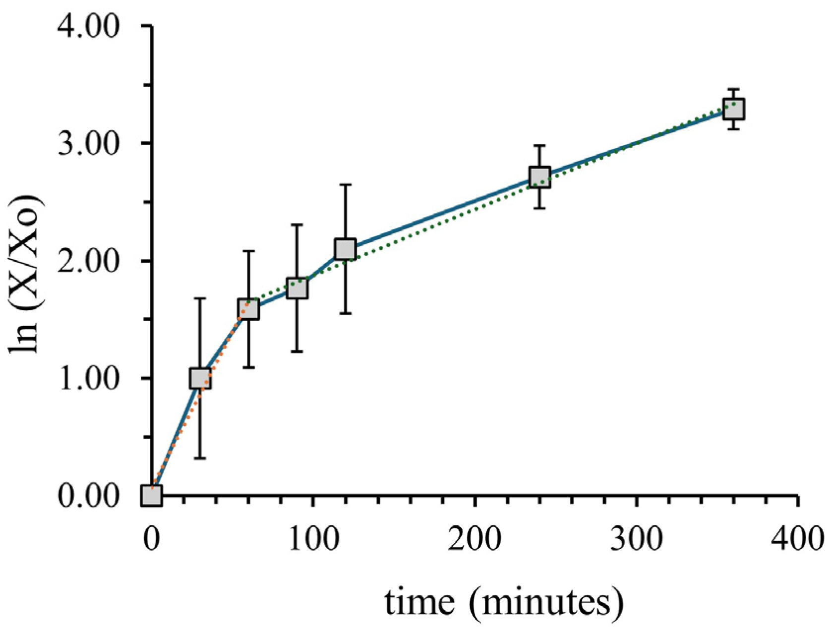
3.1. Growth Phases over the Course of the Experiment

Figure 1 shows the growth curve for SA6538 cells. The data are presented as a semi-log plot. The same data are plotted on a linear scale in Figure S12. In semi-log plots, log growth is evident as a straight line. Figure 1 demonstrates that the early growth of SA6538 cells occurs at two rates: growth is faster from 0 to 60 min (average doubling time, t_d = 33 ± 11 min) and is consistently logarithmic at a slower rate from ~60 min after inoculation (average doubling time, t_d = 132 ± 27 min). This pattern of growth is characteristic of bacteria growing in a medium containing multiple carbon sources such as LB broth. Simple sugars are the preferred energy source and are consumed first, whereas secondary substrates, including amino acids and complex carbohydrates, are consumed later. The amount of glucose present in LB broth is estimated to be less than 100 mM, and bacterial growth primarily derives from the available amino acids [21].

The data in Figure 1 show no lag phase, which is expected when inoculating overnight-grown cells into fresh, identical media [22]. In contrast, Kochan et al. claimed a lag phase of up to 120 min for similar cells grown under similar conditions. The terms “lag” phase and “log” phase were used in this previous work to differentiate cellular growth between 30–120 and 240–360 min, respectively. Based on the data in Figure 1, we will refer to the “early” and “late” log phases of growth, rather than the “lag” or “log” phases, respectively.

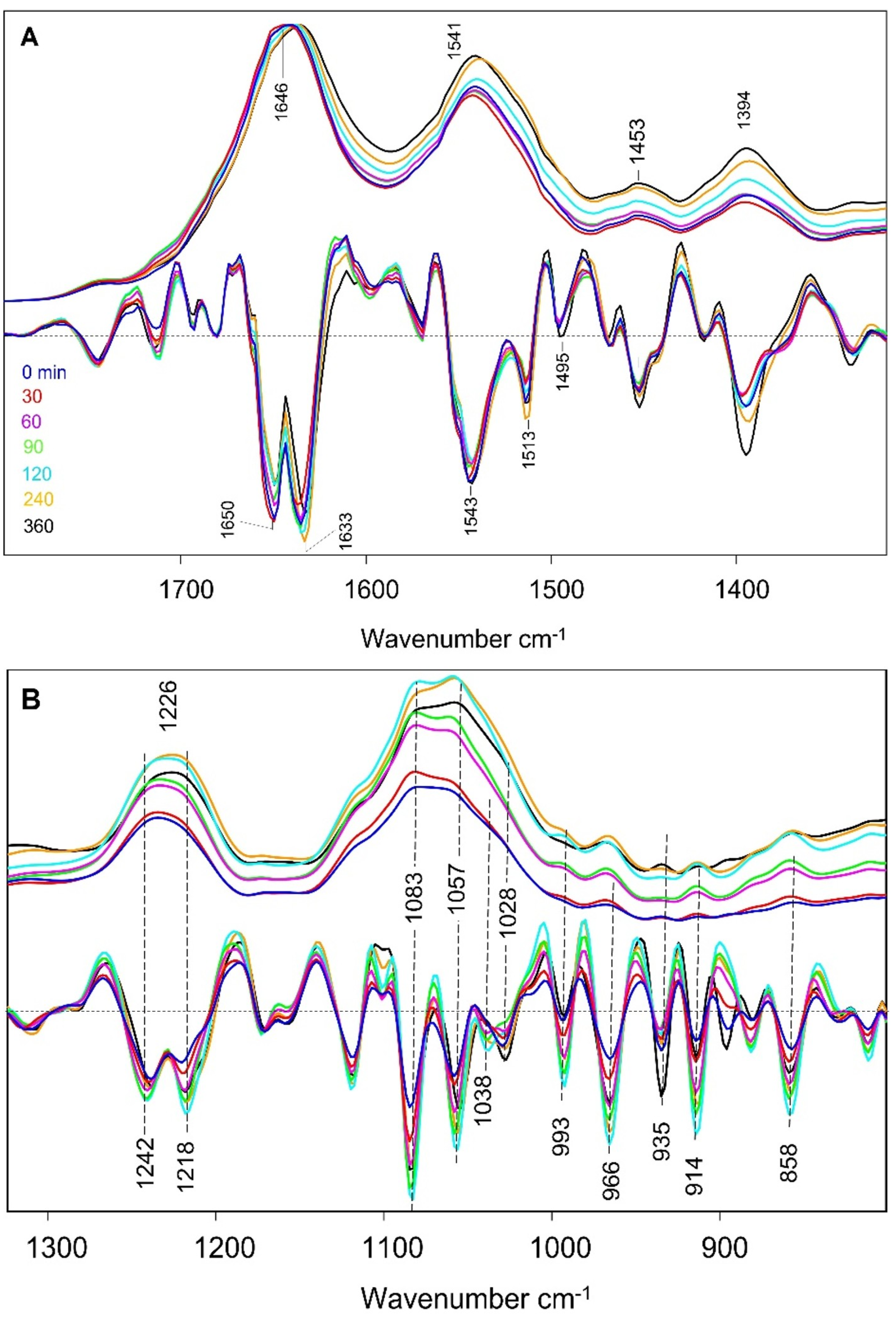
3.2. ATR-FTIR Absorption Spectra

In the following section, bands at various frequencies will be discussed. Bands at different frequencies have been associated with various subcellular biomolecular components. A listing of potential spectral band assignments is given in Table S1. The data in Table S1 are amalgamated from several sources [3,23,24,25,26,27].

Figure 2 shows ATR-FTIR absorption spectra for the cells collected at various times post-inoculation, from 0 to 360 min. The absorption spectra were subjected to a min–max normalization in the 1800–1600 cm⁻¹ region, with the maximum being near 1650 cm⁻¹.

The area under the amide II band near 1550 cm⁻¹ is similar in all seven spectra (see also baseline-corrected spectra in Figure S2), so we expected that this normalization would give a measure of cellular biomolecules relative to total protein concentration. There may be some broad baseline variations in the absorption spectra in Figure 2. Rather than apply a baseline correction procedure, which can lead to problems in spectral analysis [28], we simply removed these spectrally broad baseline features by taking the second derivative of the absorption spectra. An analysis of second derivative spectra in FTIR studies of bacteria is becoming standard [3,20,29,30]. In OPUS 7.5 software from Bruker Optics, a 9-point smoothing algorithm is automatically applied when calculating second-derivative spectra. We deemed such a smoothing acceptable, leading to minimal information loss, especially below 1600 cm⁻¹. Note that no ATR correction was applied to the absorption spectra in Figure 2. This was our preferred approach, as there may be issues or questions on the appropriateness of the ATR correction algorithms [31,32]. For completeness, we show ATR-corrected spectra in Figure S3, which can be compared to the data in Figure 2.

Spectra were collected in triplicate for three independently prepared samples, and the three spectra were averaged to produce the spectra in Figure 2. The standard error associated with the three absorption and second-derivative spectra is represented for a typical time point (30 min) in Figure S4. The error bars shown in Figure S4 are typical for the spectra at all time points.

The second-derivative spectra in Figure 2A indicate that the amide I absorption band consists of at least two underlying peaks at ~1650 and ~1633 cm⁻¹. The ratios of these two negative peaks in the second-derivative spectra vary during growth, with the 1650/1633 cm⁻¹ second-derivative peak amplitude decreasing/increasing during growth, respectively. These two amide I peaks were not observed in previous ATR-FTIR studies of a similar S. aureus strain, possibly due to limited spectral resolution [20]. Supporting this notion, Figure S5 shows the second-derivative spectra at lower spectral resolution, which indicates that the two amide I peaks merge, giving rise to a peak near 1641 cm⁻¹. Note that in the ATR-corrected spectra in Figure S3A, the amide I band displays peaks at 1656 and 1640 cm⁻¹, ~6 cm⁻¹ higher than that for the amide I peaks in Figure 2A. The intensity ratio of the two amide I peaks in the second-derivative spectra in Figure S3A is considerably altered compared to that in Figure 2A, however. Consideration of the details/complications of the ATR correction algorithm is beyond the scope of this manuscript.

The second derivative spectra in Figure 2 indicate other changes in both band intensities and frequencies as a function of cellular growth, most obviously near 1394, 1226, and 1080–1020 and in the 1000–800 cm⁻¹ region. Changes in the intensities of the negative bands in second-derivative spectra can be somewhat difficult to analyze in terms of cellular biomolecular composition, as such intensity changes do not directly relate to absorption (intensities in the second-derivative spectra are sensitive to the widths of the underlying absorption bands). Frequency shifts or disappearing/appearing bands (discussed below), on the other hand, are of greater diagnostic value, especially for spectral discrimination using a variety of statistical methodologies.

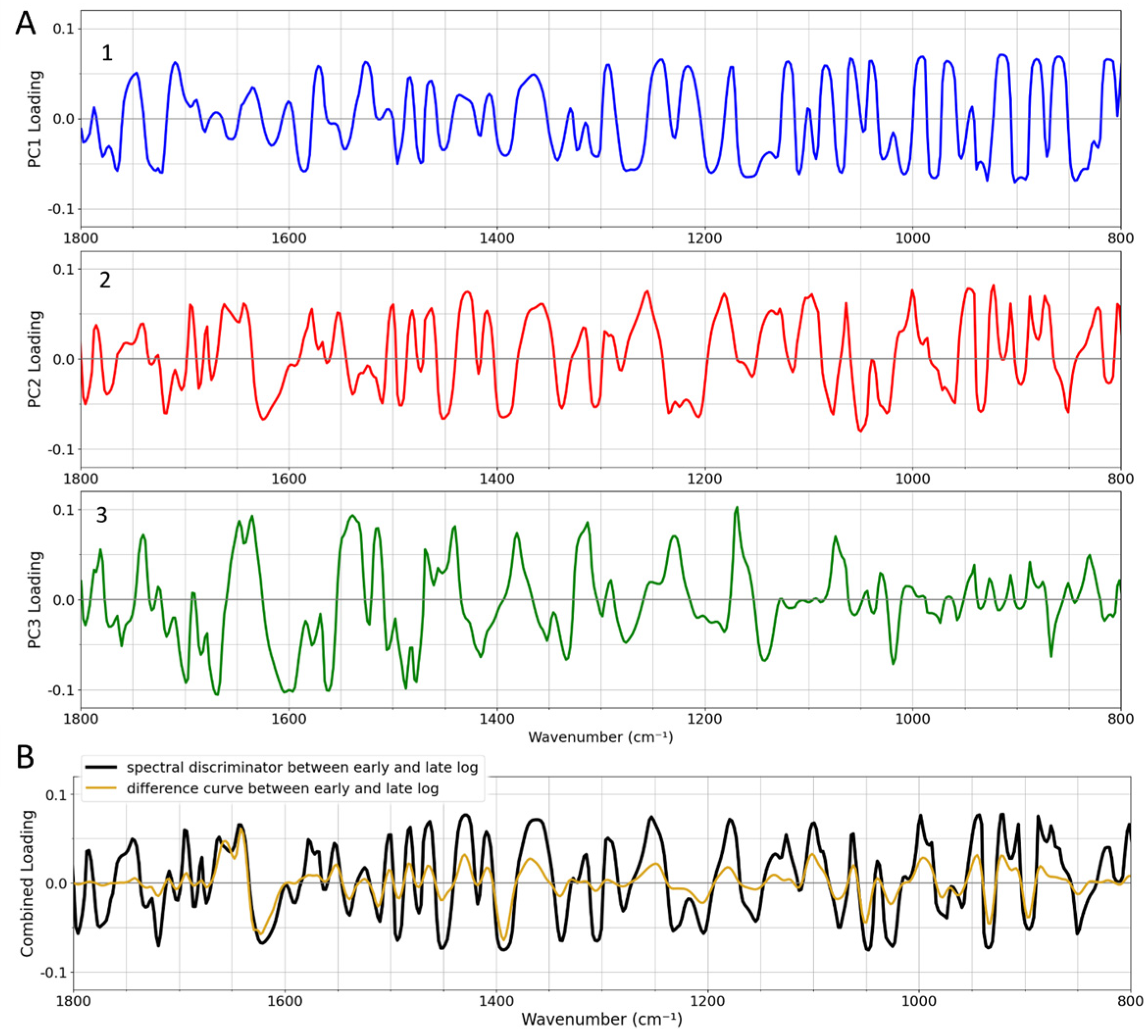
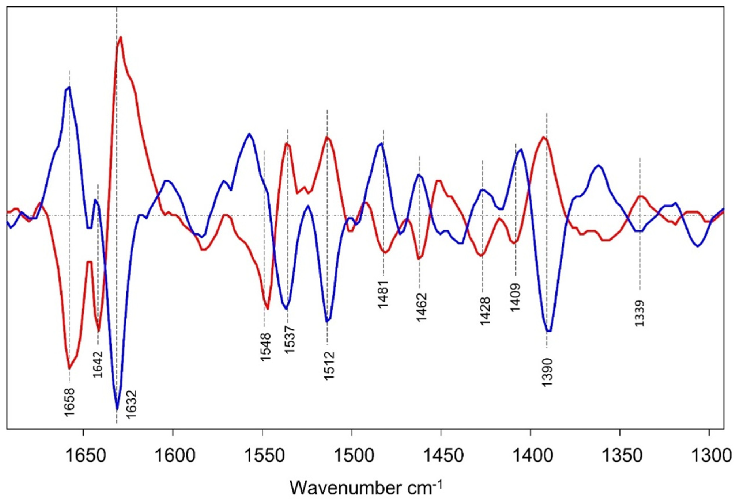
3.3. Spectral Alterations on Going from the Early to Late Log Phase

To compress the quantity of data to be analyzed and to provide a broader overview, we focus on spectra associated with cells that are mostly in the early or late exponential phase of growth. Figure 3 shows a comparison between the average ATR-FTIR spectra of bacteria in early (30–120 min) and late (240–360 min) log phases. Figure 3 indicates that differences can be seen in the second-derivative spectra between early and late log phases. These differences are more easily visualized in the “early-minus-late” difference spectrum that is also shown in Figure 3. Corresponding spectra obtained from absorption spectra that have been ATR corrected are shown in Figure S6.

The positive and negative bands in the early–late second-derivative difference spectrum are low in intensity (relative to the bands in the second-derivative spectra), and it is necessary to verify that any discussed bands have intensities that are above the noise level. The first approach to estimating the error is to calculate the standard error associated with the early and late phase spectra (average of four or two spectra, respectively). From this, the propagated error in the early-minus-late difference spectrum can be calculated. The early-minus-late difference spectrum with the associated propagated error is shown in Figure S7. Any bands discussed in this manuscript have an intensity that is above that of the error bars (see Figure S7). We have also calculated an early-minus-late difference spectrum where the early phase spectrum is represented only by the spectrum collected at 240 min (Figure S11). The results/observations derived for the main peaks discussed in this manuscript are the same when only the 240 min difference spectrum is used to represent cells in the late log phase, however.

Much information can be gleaned from the early–late difference spectrum, which shows features near 1658 and 1642 cm⁻¹ disappearing in the early-phase second-derivative spectrum and features near 1628 and 1622 cm⁻¹ appearing in the late-phase second-derivative spectrum (Figure 3A). Features at 1658 and 1642 cm⁻¹ are usually associated with protein α-helix secondary structure elements, while features near 1628 and 1622 cm⁻¹ are associated with protein β-sheet secondary structures (Table S1). Given the changes in the amide I band on going from the early to late log phase, one might expect associated changes in the amide II region near 1550 cm⁻¹. The early–late difference spectrum suggests a loss of absorption near 1553 cm⁻¹ in the early log phase and an increase in absorption near 1540 cm⁻¹ in the late log phase, again suggesting a greater degree of α-helix protein subunits in the early log phase changing to the β-sheet in the late log phase. The positive peak near 1540 cm⁻¹ in the early–late difference spectrum is well above the noise level, but a negative peak near 1553 cm⁻¹ is less obvious (Figure S7A).

In previous studies on a similar bacterial strain [20], no changes were observed in the amide I region on going from the early to late log phase. This is in spite of the fact that amide II absorption changes were observed.

In the early–late difference spectrum obtained from the ATR-corrected spectra (Figure S6A), two negative peaks are observed at 1657 and 1644 cm⁻¹ indicating a loss of features at these frequencies on going from the early to late log phase, while two positive peaks at 1632 and 1624 cm⁻¹ are also observed, indicating the appearance of peaks at these frequencies on going from early to late log phases. The interpretations of the amide I changes demonstrated in the early–late difference spectra are therefore similar, whether or not an ATR correction is applied. To further probe changes in the early–late difference spectrum that may relate to the ATR correction, Figure S8 compares the early–late difference spectra obtained from spectra with and without an ATR correction. Although there are some frequency shifts and intensity differences in the early–late difference spectra obtained from the corrected and uncorrected spectra, for the most part, the difference spectra share many similarities, and similar conclusions follow from a consideration of either the corrected or uncorrected spectra. In this manuscript, we focus on the uncorrected spectra.

The second-derivative spectra in Figure 3A indicate a band near 1394 cm⁻¹ in the spectra of late log-phase cells, which is weaker in the spectra of early log-phase cells. These differences give rise to an intense positive feature at 1393 cm⁻¹ in the early–late difference spectrum (Figure 3A). The band at 1393 cm⁻¹ may be due to the CH bending vibrations of the protein methyl groups (Table S1). It is of note that the difference features in the ~2920 cm⁻¹ region (CH stretch region) are considerably weaker than those in Figure 3 and are of less diagnostic utility. An intense feature at ~1394 cm⁻¹ in the late log phase that is diminished in the early log phase was also observed previously [20]. In the ATR-corrected early–late difference spectrum, a peak is found near 1397 cm⁻¹ (Figure S6A).

The late log-phase second-derivative spectrum in Figure 3B suggests absorption near 1308 and 1282 cm⁻¹ that is lacking in the lag phase spectrum. These features may be due to changing polysaccharide contributions within the cells in the different phases (Table S1) [33]. Amide III absorption may also occur in this spectral region [34].

The early–late difference spectrum in Figure 3B displays a negative band at 1247 cm⁻¹, suggesting a feature near 1247 cm⁻¹ in the early log-phase second-derivative spectrum that is not present (or is shifted) in the late log-phase second-derivative spectrum. In a reverse manner, the early–late difference spectrum shows a positive band near 1203 cm⁻¹, suggesting a feature near 1203 cm⁻¹ in the late log-phase second-derivative spectrum that is not present (or is shifted) in the early log-phase second-derivative spectrum. Both the 1203 and 1247 cm⁻¹ features are above the noise level in the early–late difference spectrum (Figure S7). Amide III vibrations, and antisymmetric phosphate vibrations, are known to occur near 1247 and 1203 cm⁻¹, respectively (Table S1), and may account for these features. Given the opposite behavior of the features at 1247 and 1203 cm⁻¹, if they can be assigned to amide III protein secondary structures [34], then the 1247 cm⁻¹ feature would be due to α-helical segments, while the 1215 cm⁻¹ feature would be due to β-sheet segments. This hypothesis agrees with the changes in the amide I and II spectral regions noted above, when going from the early to late log phases.

A negative band is observed near 1028 cm⁻¹ in the late log-phase second-derivative spectrum but is diminished in the early log-phase second-derivative spectrum (Figure 3B). This 1028 cm⁻¹ band may be due to the synthesis of polysaccharides (Table S1) in the late log phase, corresponding to an increase in the polysaccharide-to-protein ratio when going from the early to late log phases. Similarly, negative bands are observed at 935 and 896 cm⁻¹ in the late log-phase second-derivative spectrum but are diminished in the early log-phase second-derivative spectrum.

In a previous study on similar samples [20], an intense feature was observed at 1032 cm⁻¹ for early log-phase cells and was diminished in the spectrum of late log-phase cells. This behavior is opposite to our observations for the 1028 cm⁻¹ feature (Figure 3B).

Interestingly (for diagnostic purposes), an intense band is observed near 993 cm⁻¹ in the early log-phase second-derivative spectrum but is diminished in the late log-phase spectrum. A similar behavior is observed for a feature at 914 and 881 cm⁻¹. This behavior is opposite to that of the 1028, 935, and 896 cm⁻¹ features on going from the early to late log phases. The 993 cm⁻¹ band may be due to polysaccharides or ribose sugars of nucleic acids (Table S1).

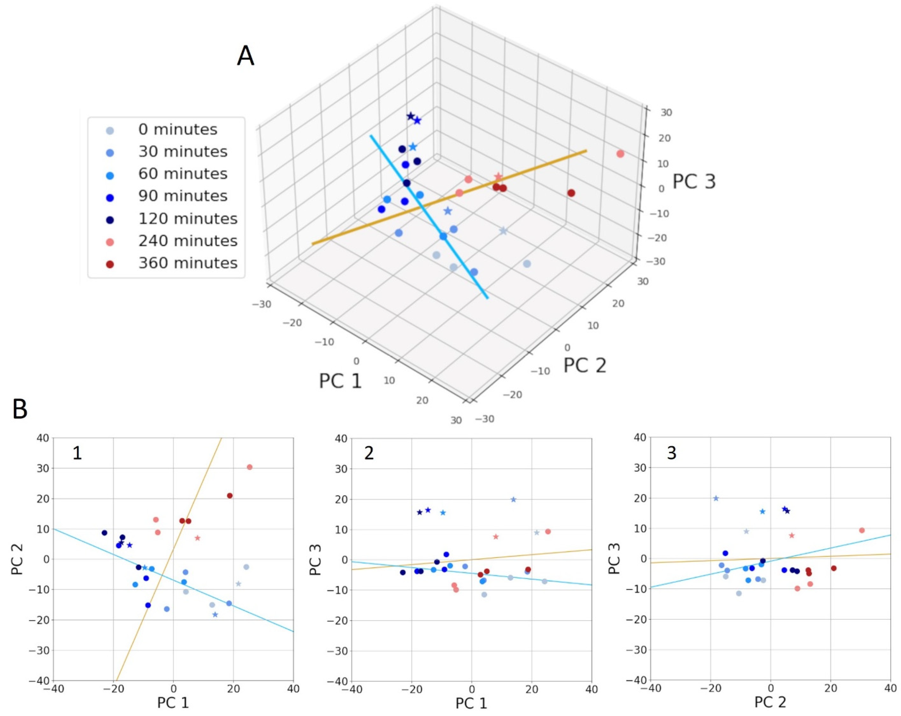
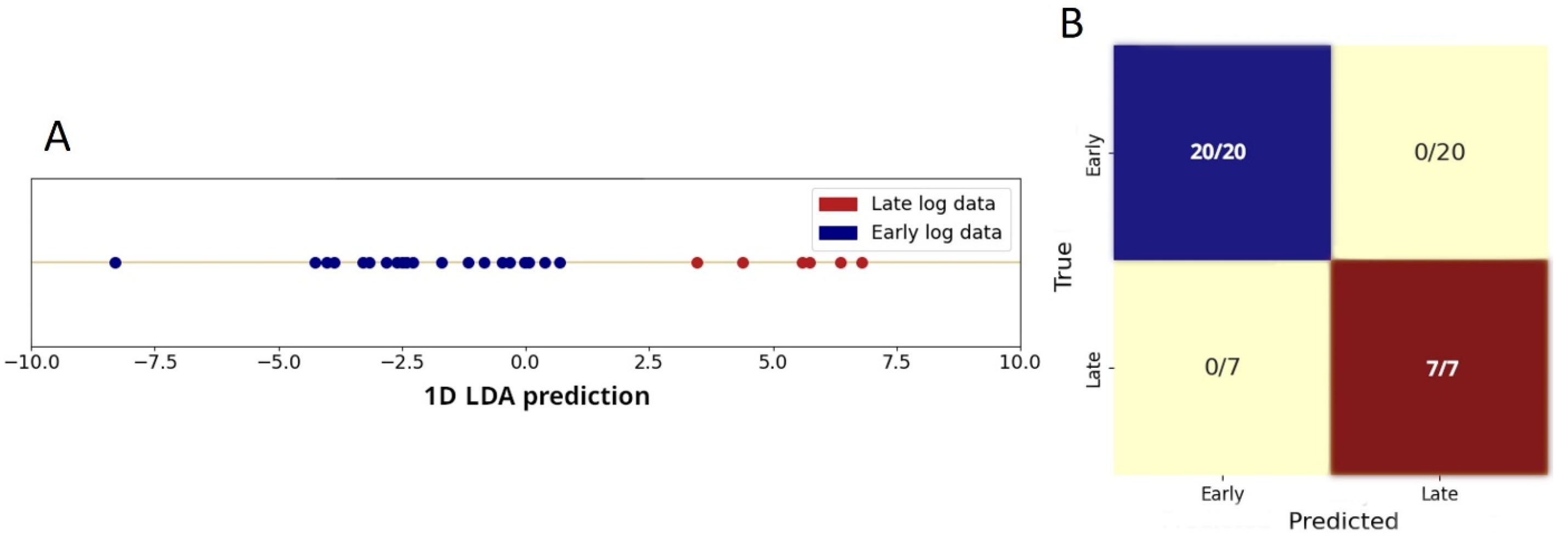
Statistical Analysis to Discriminate Spectra of Cells During Log-Phase Growth

The clear visual differences in the presence or absence of bands between the early and late log-phase spectra suggest that a statistical analysis would readily distinguish between these two growth stages. Furthermore, statistical analysis can identify the specific frequencies that provide the highest diagnostic value in differentiating the spectra of cells during growth. A 3D plot of the first three PCs is shown in Figure 4A and demonstrates that spectra associated with cells in the early and late log phases of growth cluster separately and are distinguishable. The separation is particularly obvious in a 2D plot of PC1 and PC2 (Figure 4(B1)). In Figure 4, the early log-phase data are shown as progressively darker shades of blue as time progresses. These data clearly demonstrate a temporal trend. This trend is highlighted as progressing along the direction of the blue line in Figure 4. That is, the blue line indicates the direction of maximum variance of temporal changes in the early log phase. A similar trend is also evident for the late log phase (red dots). The orange line in Figure 4 indicates the direction of maximum variance between the spectra in early and late log phases.

To connect the PCA data (Figure 4) with the early–late difference spectra in Figure 3, we analyze the PC loadings. These loadings, calculated as the elements of each eigenvector associated with each PC, are shown in Figure 5A. They highlight the frequencies that are important for each PC. The loadings together can help to assess frequencies of particular importance. The orange line in Figure 4 represents the optimal combination of PCs for separating early and late log-phase spectra. This direction of maximum separation was determined by calculating the centroids of both classes and identifying the line in 3D PC space that connects the centroids. The so-called “spectral discriminator” in Figure 5B is a linear combination of the three loadings, indicating the frequencies most relevant for discriminating the two phases. This discriminator simplifies the identification of key frequencies and is more robust to small changes in the data compared to individual loadings. The peaks in the spectral discriminator largely align with those in the early–late difference spectrum, confirming that this statistical approach supports the visual distinctions observed in the spectra.

Both PCA and visual inspection demonstrate that early and late log-phase spectra can be effectively separated. To quantify this separation, we performed Linear Discriminant Analysis (LDA). Figure 6A shows the LDA results, which provide a linear separator capable of classifying spectra as belonging to the early or late log phase. The confusion matrix in Figure 6B, generated using leave-one-out cross-validation, shows a 100% classification accuracy, confirming the effectiveness of the LDA model.

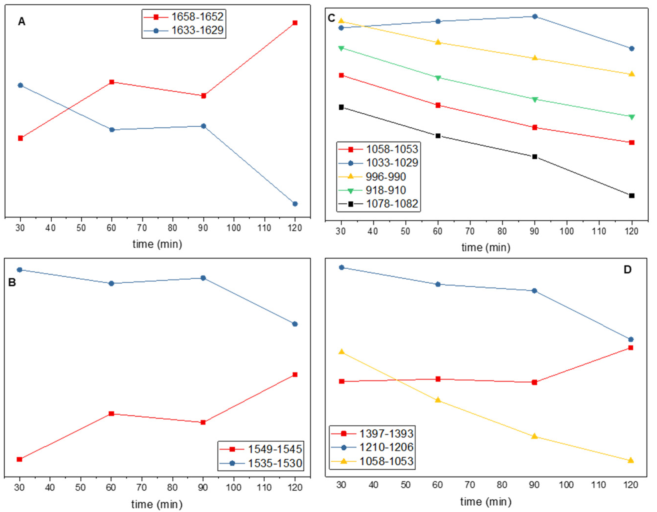
3.4. Alterations of the Spectra for Cells During the Early Log Phase of Growth

The second-derivative spectra of cells at 30, 60, 90, and 120 min after inoculation, within the early log phase, are shown in Figure 7. These are the four spectra that were averaged to produce the early log-phase spectrum discussed above. Also shown are the difference spectra calculated by subtracting the 60 min spectrum from the 30 min spectrum, the 90 min spectrum from the 60 min spectrum, and the 120 min spectrum from the 90 min spectrum. These difference spectra allow one to focus on spectral features that change during the different time intervals. An expanded view of the difference spectra with error bars is shown in Figure S9. A magnified view of the difference spectra in the amide I and II regions is shown in Figure S10.

The time-resolved difference spectra in Figure 7A demonstrate prominent changes in the amide I and II spectral regions, with the largest changes occurring in the 30–60 and 90–120 min time intervals (Figure S10). Amide I and II changes are minor in the 60–90 min time interval. In fact, Figure S9 demonstrates that the error bars in the 60–90 min difference spectrum are as large or larger than any of the difference features. So, the 60 and 90 min second-derivative spectra are identical within the limits set by the error bars in Figure S9.

The kinetics of the absorption changes in the amide I region, averaged over the 1658–1652 and 1633–1629 cm⁻¹ regions, are shown in Figure 8A. We will refer to these features (and subsequent features) as being in the middle of the range, so at 1655 and 1631 cm⁻¹, respectively. It is clear from the data in Figure 8A that the 1655 and 1631 cm⁻¹ features display opposite temporal behavior over the 30–120 min time interval, and that the changes are mostly occurring in the 30–60 and 90–120 min time intervals, as also suggested by the data in Figure 7. As indicated earlier, the kinetics associated with the 1655 and 1631 cm⁻¹ features are associated with the loss of α-helix absorption and concomitant rise in β-sheet absorption.

Given the time-resolved data in the amide I region (Figure 8A), one might expect to observe the corresponding types of temporal evolution of features in the amide II region. Figure 8B shows the kinetics of absorption changes in the amide II region at 1547 and 1533 cm^–1. Comparing the data in Figure 8A,B indicates that features at 1655 and 1547 cm⁻¹ evolve similarly. The features at 1631 and 1533 cm⁻¹ also evolve similarly. So, the 1655 and 1547 cm⁻¹ features can be associated with α-helix, while changes at 1631 and 1533 cm⁻¹ can be associated with β-sheet structures.

For many of the negative bands in the second-derivative spectra in Figure 7B, covering the ~1250−800 cm⁻¹ region, their amplitude increases continuously over the growth period considered (30–120 min). This manifests itself as many similarities in the three difference spectra in Figure 7B. The time evolution of the changes at 1056, 993, and 914 cm⁻¹ is shown in Figure 8C and demonstrates a continuous absorption increase (increasing negative intensity in the second derivative) over the 30–120 min period. This continuous increase over time is also seen in Figure S3. The time evolution of the feature at 1031 cm⁻¹ clearly differs from the other features in Figure 8C. The altered kinetics near 1031 cm⁻¹ compared to the other features in Figure 8C can also be visualized in the data in Figure 7B. In this way, the time evolution of the absorption changes can be a helpful tool to aid in spectral feature correlation and assignment.

The time evolution of the features at 1395 and 1208 cm⁻¹ is shown in Figure 8D. The time evolution of these features resembles the features in Figure 8B, suggesting that the 1395 and 1208 cm⁻¹ features are related to α-helical and β-sheet protein structures.

The absorption or second-derivative spectra indicate protein bands shifting in frequency as secondary structures are altered during growth. There is little change in the overall intensity of the broad amide I and II bands, however (Figure S3). This is not the case for non-protein bands, which do increase continuously in intensity over the 30–120 min time interval (Figure 7B). Since the spectra are roughly normalized to the amide I and II peaks, the observed changes indicate that the ratio of the cellular protein to other biomolecules decreases during early exponential growth. This change in biomolecular distributions relative to protein content is clear in the baseline-corrected absorption spectra that are shown in Figure S2.

Figure 9 compares 0–30 min and 90–120 min difference spectra in the 1700–1300 cm⁻¹ region. Many of the peaks in the two difference spectra appear to be inversely correlated (anticorrelated), indicating that biomolecular adaptations in the early log phase are reversed as the cells approach the late log phase of growth. Further investigation using a multi-omics strategy will be required to resolve the specific changes in cellular biochemistry and molecular genetics contributing to these substantial differences [19]. The differences correlate with both shifts in the availability of labile sugars in the growth medium to more complex substrates and also an increase in the S. aureus population density, which triggers density-dependent regulated adaptations via quorum sensing, i.e., bacterial cell–cell signaling by the exchange of post-translationally modified oligopeptides, or “pheromones” [35].

Since protein spectral features, such as amide I and II, invert in each of the difference spectra, this suggests a method for the qualitative identification of protein spectral features outside of the amide I and II regions (the time-resolved data in Figure 8 also indicate a method for distinguishing protein features from that of other cellular components). The most obvious or most intense inversion feature between the two difference spectra outside of the amide I or II regions is observed at ~1390 cm⁻¹. The absorption changes at 1395 cm⁻¹ are shown in Figure 8D and demonstrate temporal features that are most similar to those of α-helical protein segments. Above, it was suggested that α-helical protein segments could be exhibited near 1390 cm⁻¹. Other inverted difference features in Figure 6 are observed at 1512, 1462, 1428, and 1339 cm⁻¹, also suggesting a contribution from protein modes at these frequencies.

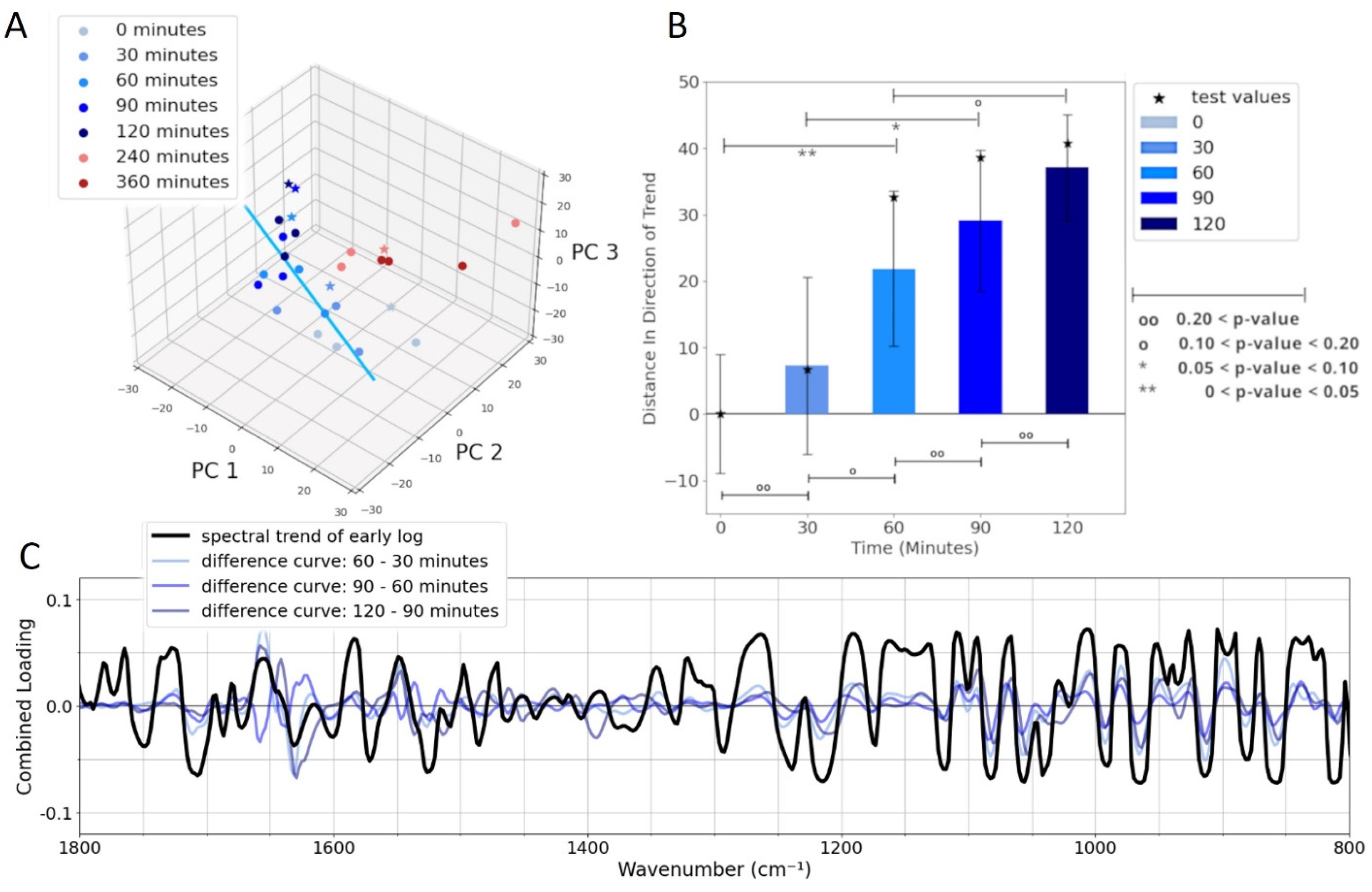
3.5. Statistical Analysis of Spectra for Cells During Early Log-Phase Growth

In the 3D PC space with the first three PCs (Figure 4A), we project all the blue data points (cells during early log phase) onto the blue trend line and measure their distance from the point at time zero. The result, shown in Figure 10A, reflects how the spectra follow the temporal trend. Statistically significant differences are observed between the spectra at 0 and 60 min (p-values < 0.05) and between 30 and 90 min (p-values < 0.1). However, no significant difference is detected between the spectra at 60 and 120 min. These results indicate that the most significant spectral (and likely biomolecular) changes occur within the first 60 to 90 min after inoculation. Additionally, no significant differences are found in spectral data from time points 30 min apart.

To connect these findings with the biochemical changes in the cells, we revisit the loading plot. In Figure 10B, a different linear combination of loadings is used, corresponding to the direction of the trend (blue line in Figure 4A). This projection (thick black line in Figure 10C) highlights new peaks, allowing us to identify the FTIR frequencies that drive the trend.

4. Conclusions

Dynamic ATR-FTIR difference spectroscopy is demonstrated to be a powerful tool to probe the changing biochemical composition of bacteria during cellular growth. Changes in molecular composition occurring during exponential growth are identified, and we show that we can probe such changes in as little as 30 min.

We show from the statistical analysis of the spectral data that cells in the early or late exponential phase can be discriminated with 100% accuracy. The trend in the spectral data for cells within the early exponential phase can also be discriminated with high accuracy.

We show how spectral features associated with different protein secondary structural elements evolve over time. Different secondary structural elements evolve differently, indicating interconversion between secondary structures during growth. Protein spectral features are shown to evolve differently from carbohydrate or nucleic acid spectral features. These different types of time evolutions can be used as an aid in spectral band assignments, and we suggest assignments for some of the bands in the spectra based on temporal evolution.

Finally, with the current work in place, we pave the way for identifying growth abnormalities in studies of bacterial cells in the presence of antibiotics or other types of inhibitors or environmental perturbations. Such abnormalities will report on the susceptibility of the bacteria to the perturbation.

References

1. AlMasoud, N.; Muhamadali, H.; Chisanga, M.; AlRabiah, H.; Lima, C.A.; Goodacre, R. Discrimination of bacteria using whole organism fingerprinting: The utility of modern physicochemical techniques for bacterial typing. Analyst 2021, 146, 770–788. [Google Scholar] [CrossRef] [PubMed]
2. Novais, Â.; Freitas, A.R.; Rodrigues, C.; Peixe, L. Fourier transform infrared spectroscopy: Unlocking fundamentals and prospects for bacterial strain typing. Eur. J. Clin. Microbiol. Infect. Dis. 2019, 38, 427–448. [Google Scholar] [CrossRef] [PubMed]
3. Kassem, A.; Abbas, L.; Coutinho, O.; Opara, S.; Najaf, H.; Kasperek, D.; Pokhrel, K.; Li, X.; Tiquia-Arashiro, S. Applications of Fourier Transform-Infrared spectroscopy in microbial cell biology and environmental microbiology: Advances, challenges, and future perspectives. Front. Microbiol. 2023, 14, 1304081. [Google Scholar]
4. Veettil, T.C.P.; Kochan, K.; Williams, G.C.; Bourke, K.; Kostoulias, X.; Peleg, A.Y.; Lyras, D.; De Bank, P.A.; Perez-Guaita, D.; Wood, B.R. A Multimodal Spectroscopic Approach Combining Mid-infrared and Near-infrared for Discriminating Gram-positive and Gram-negative Bacteria. Anal. Chem. 2024, 96, 18392–18400. [Google Scholar]
5. Novais, Â.; Gonçalves, A.B.; Ribeiro, T.G.; Freitas, A.R.; Méndez, G.; Mancera, L.; Read, A.; Alves, V.; López-Cerero, L.; Rodríguez-Baño, J.; et al. Development and validation of a quick, automated, and reproducible ATR FT-IR spectroscopy machine-learning model for Klebsiella pneumoniae typing. J. Clin. Microbiol. 2024, 62, e01211-23. [Google Scholar] [CrossRef]
6. Bertrand, R.L. Lag Phase Is a Dynamic, Organized, Adaptive, and Evolvable Period That Prepares Bacteria for Cell Division. J. Bacteriol. 2019, 201, 10–1128. [Google Scholar] [CrossRef]
7. Rolfe, M.D.; Rice, C.J.; Lucchini, S.; Pin, C.; Thompson, A.; Cameron, A.D.S.; Alston, M.; Stringer, M.F.; Betts, R.P.; Baranyi, J.; et al. Lag Phase Is a Distinct Growth Phase That Prepares Bacteria for Exponential Growth and Involves Transient Metal Accumulation. J. Bacteriol. 2012, 194, 686–701. [Google Scholar] [CrossRef]
8. Widdel, F. Theory and measurement of bacterial growth. Dalam Grund. Mikrobiol. 2007, 4, 1–11. [Google Scholar]
9. Swinnen, I.A.M.; Bernaerts, K.; Dens, E.J.J.; Geeraerd, A.H.; Van Impe, J.F. Predictive modelling of the microbial lag phase: A review. Int. J. Food Microbiol. 2004, 94, 137–159. [Google Scholar] [CrossRef]
10. Eymann, C.; Dreisbach, A.; Albrecht, D.; Bernhardt, J.; Becher, D.; Gentner, S.; Tam, L.T.; Büttner, K.; Buurman, G.; Scharf, C.; et al. A comprehensive proteome map of growing Bacillus subtilis cells. Proteomics 2004, 4, 2849–2876. [Google Scholar] [CrossRef]
11. Kumar, V.; Ahluwalia, V.; Saran, S.; Kumar, J.; Patel, A.K.; Singhania, R.R. Recent developments on solid-state fermentation for production of microbial secondary metabolites: Challenges and solutions. Bioresour. Technol. 2021, 323, 124566. [Google Scholar] [CrossRef] [PubMed]
12. Siegele, D.A.; Kolter, R. Life after log. J. Bacteriol. 1992, 174, 345–348. [Google Scholar] [CrossRef] [PubMed]
13. Overton, T.W. Recombinant protein production in bacterial hosts. Drug Discov. Today 2014, 19, 590–601. [Google Scholar] [CrossRef] [PubMed]
14. San-Miguel, T.; Pérez-Bermúdez, P.; Gavidia, I. Production of soluble eukaryotic recombinant proteins in E. coli is favoured in early log-phase cultures induced at low temperature. Springerplus 2013, 2, 89. [Google Scholar] [CrossRef]
15. Mitsakakis, K.; Kaman, W.E.; Elshout, G.; Specht, M.; Hays, J.P. Challenges in identifying antibiotic resistance targets for point-of-care diagnostics in general practice. Future Microbiol. 2018, 13, 1157–1164. [Google Scholar] [CrossRef]
16. Centers_for_Disease_Control. COVID-19: U.S. Impact on Antimicrobial Resistance, Special Report 2022; CDC: Atlanta, GA, USA, 2022. [Google Scholar]
17. Haaber, J.; Cohn, M.T.; Frees, D.; Andersen, T.J.; Ingmer, H. Planktonic aggregates of Staphylococcus aureus protect against common antibiotics. PLoS ONE 2012, 7, e41075. [Google Scholar] [CrossRef]
18. Zhang, M.; Michie, K.L.; Cornforth, D.M.; Dolan, S.K.; Wang, Y.; Whiteley, M. Impact of Growth Rate on the Protein-mRNA Ratio in Pseudomonas aeruginosa. mBio 2023, 14, e0306722. [Google Scholar] [CrossRef]
19. Chaffin, D.O.; Taylor, D.; Skerrett, S.J.; Rubens, C.E. Changes in the Staphylococcus aureus transcriptome during early adaptation to the lung. PLoS ONE 2012, 7, e41329. [Google Scholar] [CrossRef]
20. Kochan, K.; Lai, E.; Richardson, Z.; Nethercott, C.; Peleg, A.Y.; Heraud, P.; Wood, B.R. Vibrational Spectroscopy as a Sensitive Probe for the Chemistry of Intra-Phase Bacterial Growth. Sensors 2020, 20, 3452. [Google Scholar] [CrossRef]
21. Sezonov, G.; Joseleau-Petit, D.; D’Ari, R. Escherichia coli physiology in Luria-Bertani broth. J. Bacteriol. 2007, 189, 8746–8749. [Google Scholar] [CrossRef]
22. Jones, E.W.; Derrick, J.; Nisbet, R.M.; Ludington, W.B.; Sivak, D.A. First-passage-time statistics of growing microbial populations carry an imprint of initial conditions. Sci. Rep. 2023, 13, 21340. [Google Scholar] [CrossRef] [PubMed]
23. Schmitt, J.; Flemming, H.C. FTIR-spectroscopy in microbial and material analysis. Int. Biodeterior. Biodegrad. 1998, 41, 1–11. [Google Scholar] [CrossRef]
24. Barth, A. Infrared spectroscopy of proteins. Biochim. Biophys. Acta BBA Bioenerg. 2007, 1767, 1073–1101. [Google Scholar] [CrossRef] [PubMed]
25. Movasaghi, Z.; Rehman, S.; Rehman, D.I.U. Fourier Transform Infrared (FTIR) Spectroscopy of Biological Tissues. Appl. Spectrosc. Rev. 2008, 43, 134–179. [Google Scholar] [CrossRef]
26. Kochan, K.; Bedolla, D.E.; Perez-Guaita, D.; Adegoke, J.A.; Veettil, T.C.P.; Martin, M.; Roy, S.; Pebotuwa, S.; Heraud, P.; Wood, B.R. Infrared Spectroscopy of Blood. Appl. Spectrosc. 2021, 75, 611–646. [Google Scholar] [CrossRef]
27. Yang, H.; Shi, H.; Feng, B.; Wang, L.; Chen, L.; Alvarez-Ordóñez, A.; Zhang, L.; Shen, H.; Zhu, J.; Yang, S.; et al. Protocol for bacterial typing using Fourier transform infrared spectroscopy. STAR Protoc. 2023, 4, 102223. [Google Scholar] [CrossRef]
28. Zhang, F.; Tang, X.; Tong, A.; Wang, B.; Wang, J. An Automatic Baseline Correction Method Based on the Penalized Least Squares Method. Sensors 2020, 20, 2015. [Google Scholar] [CrossRef]
29. Grunert, T.; Wenning, M.; Barbagelata, M.S.; Fricker, M.; Sordelli, D.O.; Buzzola, F.R.; Ehling-Schulz, M. Rapid and Reliable Identification of Capsular Serotypes by Means of Artificial Neural Network-Assisted Fourier Transform Infrared Spectroscopy. J. Clin. Microbiol. 2013, 51, 2261–2266. [Google Scholar] [CrossRef]
30. Kochan, K.; Nethercott, C.; Taghavimoghaddam, J.; Richardson, Z.; Lai, E.; Crawford, S.A.; Peleg, A.Y.; Wood, B.R.; Heraud, P. Rapid Approach for Detection of Antibiotic Resistance in Bacteria Using Vibrational Spectroscopy. Anal. Chem. 2020, 92, 8235–8243. [Google Scholar] [CrossRef]
31. Lee, L.C.; Liong, C.-Y.; Jemain, A.A. A contemporary review on Data Preprocessing (DP) practice strategy in ATR-FTIR spectrum. Chemom. Intell. Lab. Syst. 2017, 163, 64–75. [Google Scholar] [CrossRef]
32. Grdadolnik, J. ATR-FTIR Spectroscopy: Its Aadvantages and Limitations. Acta Chim. Slov. 2002, 49, 631–642. [Google Scholar]
33. Wiercigroch, E.; Szafraniec, E.; Czamara, K.; Pacia, M.Z.; Majzner, K.; Kochan, K.; Kaczor, A.; Baranska, M.; Malek, K. Raman and infrared spectroscopy of carbohydrates: A review. Spectrochim. Acta Part A Mol. Biomol. Spectrosc. 2017, 185, 317–335. [Google Scholar] [CrossRef] [PubMed]
34. Cai, S.; Singh, B.R. A distinct utility of the amide III infrared band for secondary structure estimation of aqueous protein solutions using partial least squares methods. Biochemistry 2004, 43, 2541–2549. [Google Scholar] [CrossRef] [PubMed]
35. Jenul, C.; Horswill, A.R. Regulation of Staphylococcus aureus Virulence. Microbiol. Spectr. 2019, 19, 1128. [Google Scholar] [CrossRef]
Figure 1. Semi-log plot displaying bacterial growth data over a six-hour period for SA6538 cells grown in LB broth, obtained from measurements of the optical density at 600 nm. Dotted lines are linear curve fits for the 0–60 min period (orange) and 60–360 min period (green).
Spectroscj 03 00015 g001
Figure 2. Average ATR-FTIR spectra (top curves) and second-derivative spectra (bottom curves) in the (A) 1780–1320 and (B) 1320–820 cm−1 ranges for bacteria taken at various times, from 0 to 360 min, after incubation. Color coding is indicated in (A) and is the same for absorption and second-derivative spectra. Color coding is the same in both (A,B). Second-derivative spectra are scaled by a factor of 400 for an easy comparison to the absorption spectra. FTIR absorption spectra were min–max normalized with a min/max near 1800/1650 cm−1, respectively.
Spectroscj 03 00015 g002
Figure 3. Average ATR-FTIR absorption and scaled second-derivative spectra recorded for SA6358 cells in the early (blue) and late (red) log phases in the (A) 1800–1350 and (B) 1350–850 cm−1 range. An analysis of the changes in the second-derivative spectra of bacteria in the early and late log phases is also shown as an early–late difference spectrum. Early log-phase spectra are the average of four spectra collected at 30, 60, 90, and 120 min. Late log-phase spectra are the average of two spectra collected at 240 and 360 min.
Spectroscj 03 00015 g003
Figure 4. (A) Principal component analysis (PCA) of second derivative spectra collected in triplicate at 7 time points. Early and late log phases are shown in blue and red, respectively, with progressively darker shades denoting later time points. A fourth dataset (stars) was included for comparison. The orange line represents the direction of maximal separation between early and late log phases, while the blue line highlights the temporal trajectory during early log-phase growth. (B) Projections of data points and trend vectors onto each pairwise combination of principal components. The PC 1 vs. PC 2 plot demonstrates the best discrimination between early and late log phases.
Spectroscj 03 00015 g004
Figure 5. (A) Loadings of PC1 (blue), 2 (red), and 3 (green), scaled so that their sum across all frequencies is 1. (B) The spectral discriminator (black), a linear combination of the PCs, is obtained by projecting the loadings onto the direction of maximum discrimination (orange line in Figure 4A). This spectral discriminator is overlaid with the inverted early-minus-late difference spectrum from Figure 3 for comparison.
Spectroscj 03 00015 g005
Figure 6. (A) Linear Discriminant Analysis (LDA) performed on the first three PCs, projecting spectra from early (blue) to late (red) log phases onto a single axis that maximizes between-group separation while minimizing within-group separation. The resulting projection clearly distinguishes the two classes. (B) Confusion matrix from leave-one-out cross-validation, indicating 100% accuracy in classifying spectra as early or late log phases.
Spectroscj 03 00015 g006
Figure 7. Comparison of the averaged second derivative of the ATR-FTIR spectra recorded for bacterial cells within the lag phase in the (A) 1800–1180 cm−1 and (B) 1250–790 cm−1 ranges. Also shown are three difference spectra obtained by subtracting the spectrum at one time point from the spectrum at the next nearest time point.
Spectroscj 03 00015 g007
Figure 8. Time evolution of the intensity of second-derivative features. The vertical axis is arbitrary as it is the trend in the intensity changes that is relevant. As an example, the 1633–1629 cm−1 feature in panel (A) (blue) corresponds to a negative intensity in the second derivative spectra at 30 min. with the negative intensity increasing at later times. The kinetic data shown in each panel is the average of several frequencies covering the spectral ranges indicated in the legends in panels (AD). Experimentally, kinetic data was obtained approximately every 2 cm−1. So, for example, for the data covering the 1658–1652 cm−1 region, four kinetics at 1658, 1656, 1654 and 1652 cm−1 were averaged to produce the kinetic trace shown in (A) (red). The same averaging was performed to produce the kinetics in panels (BD).
Spectroscj 03 00015 g008
Figure 9. Comparison of 0–30 min (blue) and 90–120 min (red) difference spectra in the 1700–1300 cm−1 region.
Spectroscj 03 00015 g009
Figure 10. (A) PCA plot from Figure 4A with the blue line tracing the temporal trend of early log-phase spectra over time (shaded from light to dark blue). (B) Quantification of this temporal trend in PC space for early log-phase samples. Bars represent means with 90% confidence intervals. Horizontal lines indicate p-values for comparisons between 30 min and 60 min intervals, with statistical significance denoted by stars (*, 0.05 < p < 0.10; ** 0 < p < 0.05) and non-significant comparisons marked by circles (o, 0.2 > p > 0.1; oo; p > 0.2). (B) Combined PC loadings (black) projected onto the direction of the early log-phase trend (blue line from (A)). Higher values correspond to lower diagnostic relevance of the corresponding wavenumbers in capturing early log-phase dynamics. (C) Overlaid inverted difference curves (light to dark blue) from Figure 7 illustrate 30-min incremental changes in spectral features.
Spectroscj 03 00015 g010
Disclaimer/Publisher’s Note: The statements, opinions and data contained in all publications are solely those of the individual author(s) and contributor(s) and not of MDPI and/or the editor(s). MDPI and/or the editor(s) disclaim responsibility for any injury to people or property resulting from any ideas, methods, instructions or products referred to in the content.