Abstract
Forage yield estimates provide relevant information to manage and quantify ecosystem services in grasslands. We fitted and validated prediction models of forage yield for several prominent grasses used in restoration projects in semiarid areas. We used field forage harvests from three different sites in Northern Utah and Southern California, USA, in conjunction with multispectral, high-resolution UAV imagery. Different model structures were tested with simple models using a unique predictor, the forage volumetric 3D space, and more complex models, where RGB, red edge, and near-infrared spectral bands and associated vegetation indices were used as predictors. We found that for most dense canopy grasses, using a simple linear model structure could explain most (R2 0.7) of the variability of the response variable. This was not the case for sparse canopy grasses, where a full multispectral dataset and a non-parametric model approach (random forest) were required to obtain a maximum R2 of 0.53. We developed transparent protocols to model forage yield where, in most circumstances, acceptable results could be obtained with affordable RGB sensors and UAV platforms. This is important as users can obtain rapid estimates with inexpensive sensors for most of the grasses included in this study.
1. Introduction
Reliable estimates of yield for forage grasses can provide insights for the quantification of ecosystem services (i.e., carbon sequestration, water infiltration, pollination), plant breeding, as well as tools for the allocation of resources in livestock production. Grass forage yield estimates are important in ecology for several reasons. Forage grasses are a crucial source of nutrition for ruminant livestock and estimates of forage yield can help ensure an adequate feed supply, which, in turn, can increase the availability and affordability of livestock products. This is important in regions where land resources are scarce, as increasing forage yields can enable greater herd densities on existing pasture [1]. Furthermore, estimates of grass forage yields are important for the determination of the grazing capacity of a grassland ecosystem [2]. In addition, the knowledge of available forage enables land managers to make informed decisions about stocking rates and grazing management practices to prevent overgrazing and maintain the health of grasslands [3]. Yield estimates are important for understanding the relationship between climate and forage growth, as research has shown that forage yield is closely related to climatic factors such as precipitation [2]. Forage yield estimates also have implications for soil health and carbon sequestration. High-yielding forage grass cultivars with extensive root systems can contribute to increased soil organic carbon (SOC) stocks. Roots are an important input of organic matter into the soil, and cultivars bred for increased forage yield can lead to important increases in SOC. This has implications for climate-smart agriculture and the potential for grasslands to sequester carbon and mitigate climate change [4]. Moreover, understanding the forage value of different grass species and cultivars can help stockholders make informed decisions about which species to grow and how to manage their pastures [5].
Unmanned aerial vehicle (UAV) imagery has been used to model grass forage yield in semiarid landscapes through various approaches and techniques. Prediction models for dry matter yield (DMY) in temperate grasslands using UAV red, green, and blue (RGB) imaging was developed and compared to the remote sensing technique with the following two conventional methods: destructive biomass sampling and ruler height measurements. The results of the temperate grassland study showed that yield prediction by UAV RGB imaging provided similar accuracies as the ruler height measurements [6]. Agronomic parameters have also been monitored using low-cost UAV RGB imagery to observe the biophysical characteristics of winter wheat crops [7]. UAVs with higher-end sensors such as multispectral or hyperspectral imagery have been used for (a) assessing the effects of fertilizer application on yields of rice and wheat [8], (b) quantifying grassland biomass and nitrogen content [6,9], and (c) the calibration of robust yield and quality models [10]. These hyperspectral sensors are usually much more expensive than simple RGB systems. Generally, UAV imagery (RGB, multispectral, or hyperspectral) has been utilized to model accurate estimates of grass forage yield in semiarid landscapes by capturing high-resolution imagery and extracting relevant features and vegetation indices.
We modeled forage yield for several grasses that are used in dryland and irrigated pasture and restoration projects across the western USA. Grasses evaluated in our analysis include orchard grass (Dactylis glomerata L.) and tall fescue (Festuca arundinacea Schreb.). Tall fescue has been reported to reduce soil and water loss [11] and is considered one of the most important species used in phytoremediation projects [12]. We also included intermediate wheatgrass (IWG) (Thinopyrum intermedium (Host) Barkworth & D.R. Dewey), which has shown promise to enhance soil ecosystem services [13,14] and is valued as a dual-use forage and grain crop and for its ability to suppress weeds [15]. We also included drought-tolerant, perennial grass bluebunch wheatgrass (BBWG) (Pseudoroegneria spicata (Pursh) Á. Löve), which is one of the prevalent native grass species used in restoration projects in the Great Basin area of the Western USA [16] and is also known for its ability to physically stabilize and remediate contaminated sites in semiarid environments [17]. We used BBWG in this research to reflect how well a forage yield model can accommodate sparse canopy grass.
The main objectives of our research were threefold: (a) fit and validate a global model to predict forage yield for important grasses of semiarid landscapes using UAV multispectral imagery, (b) assess the strength of an affordable, photogrammetry-derived volumetric 3D space as the sole predictor of forage yield, and (c) evaluate data requirements to obtain transparent predictions in sparse canopy grasses.
2. Materials and Methods
2.1. Study Areas
Forage samples were acquired from existing grass monoculture experiments at two research farms in Northern Utah and one location in Southern California, where several grass and legume species were established (Table 1).

Table 1.
Characteristics of research sites where forage samples were collected.
2.2. Forage Data Collection
In this research, we emphasize the building of models for grasses that exhibit dense and sparse canopy architectures. The sparse canopy grass species used in this research was Bluebunch wheatgrass (BBWG) (Pseudoroegneria spicata), and the rest of the species were considered grasses with dense canopies. The main criterion used to differentiate sparse from dense canopies was the number of lignified stems in the canopy. Bunchgrasses such as BBWG, unlike sod-forming grasses (the rest of the species used here), have a crown area composed of many individual stems packed into the canopy. This structural difference raises the likelihood that bunchgrasses have more stems in the canopy compared to sod-forming grasses [18]. The growth form of bunchgrasses can also lead to the self-shading of their foliage, reducing the overall amount of the photosynthetically active leaf area [19]. Conversely, the foliage of sod-forming grasses tends to be more abundant and continuous due to their spreading (rhizomatous) nature, contributing to greater overall coverage of foliage [20] compared to bunchgrasses. In this context, the canopies of sod-forming grasses are comparatively denser (i.e., more foliage or green matter) than bunchgrasses, which, for our research purposes, was considered to have a sparse canopy.
2.2.1. Shandon, Canyon Ranch Site—California Central Coast, San Luis Obispo County—Dense Canopy Grasses
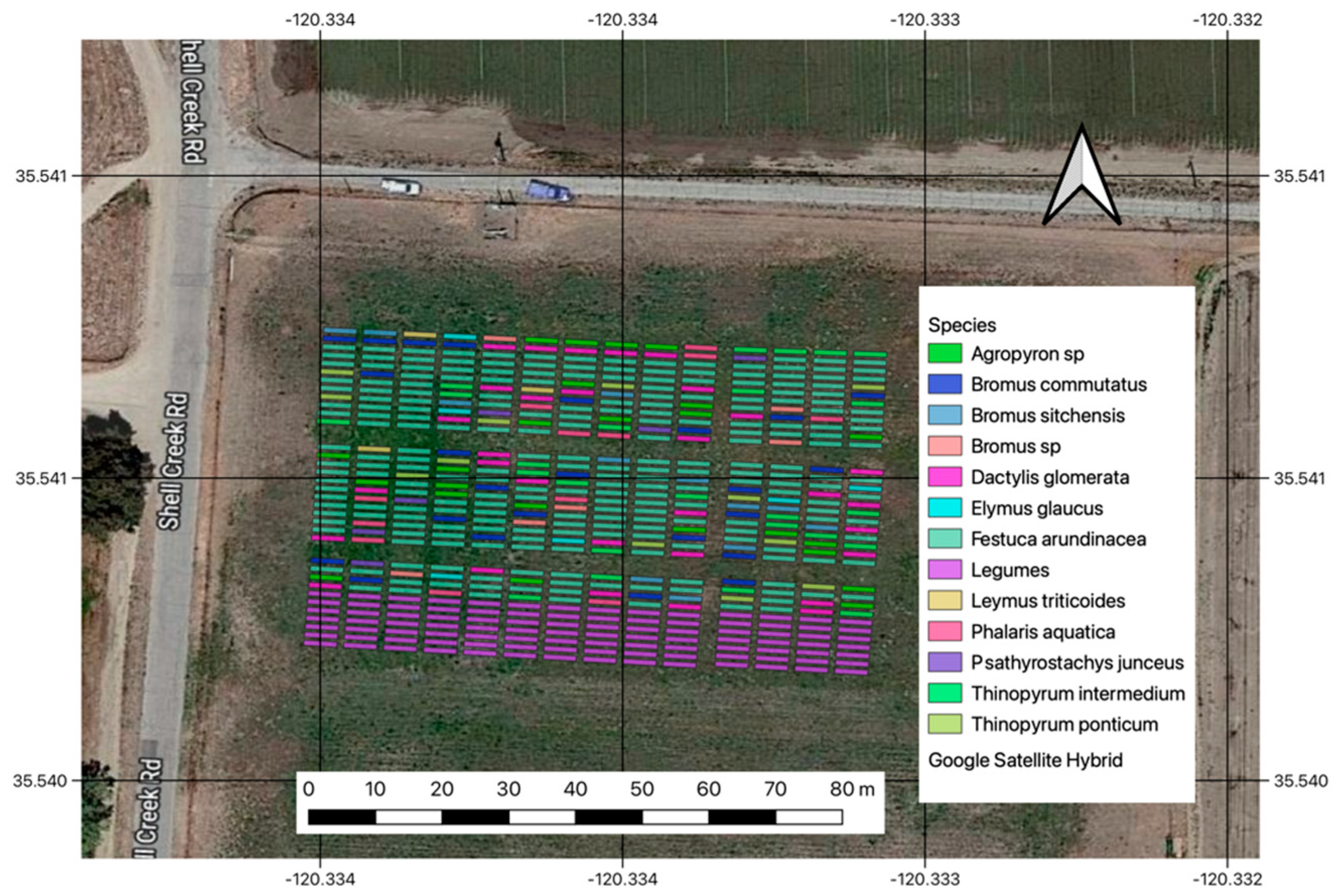
The Shandon site is located approximately 11.5 km southeast of the city of Shandon, along Shell Creek Road, California. The mean elevation at the site is 373 m.a.s.l. with an average annual temperature of 15.7 °C and 330 mm of yearly precipitation. At this site, 490 plots (dimensions 5 × 1 m) were established in 2022. A total of 12 forage grass species and several legumes (Figure 1) were planted at this site and were available for harvest. Legumes were not included in this analysis due to a considerable presence of weeds and non-desirable plant matter.

Figure 1.
Geographic location and layout of the Shandon experiment with the list of grasses that were harvested at this site. White arrow indicates North.
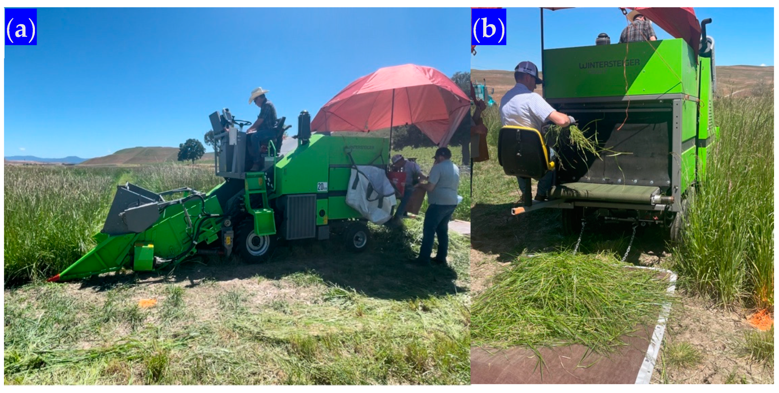
The plots were harvested in a serpentine (east to west) direction using a Wintersteiger forage harvester. In addition to cutting and picking up the green matter for each plot, the harvester recorded the total plot wet weight (kg) into an electronic spreadsheet. The harvester was equipped such that the operator could collect a representative sample from the total green matter for each plot immediately after harvest (Figure 2). The samples were placed in paper bags, and their contents were recorded as wet weight at the field. Samples were transported back to Logan, Utah, and air-dried. Dry weights for each sample were recorded subsequently. Air drying was conducted by leaving the bagged samples at the drier for several days at 60 °C until constant weights were achieved. At this site, two harvests were conducted: the first harvest in the second week of May 2023 and the second harvest in the second week of July 2023. This provided the opportunity to assess the ability of geospatial models to predict forage yield at different stages of growth for the grasses of interest.

Figure 2.
(a) Plots harvested at the Shandon site using a motorized forage harvester—the harvester records total plot weight; (b) Immediate collection of a plot-representative sample to obtain wet and dry weights back at the laboratory.
2.2.2. Richmond Farm
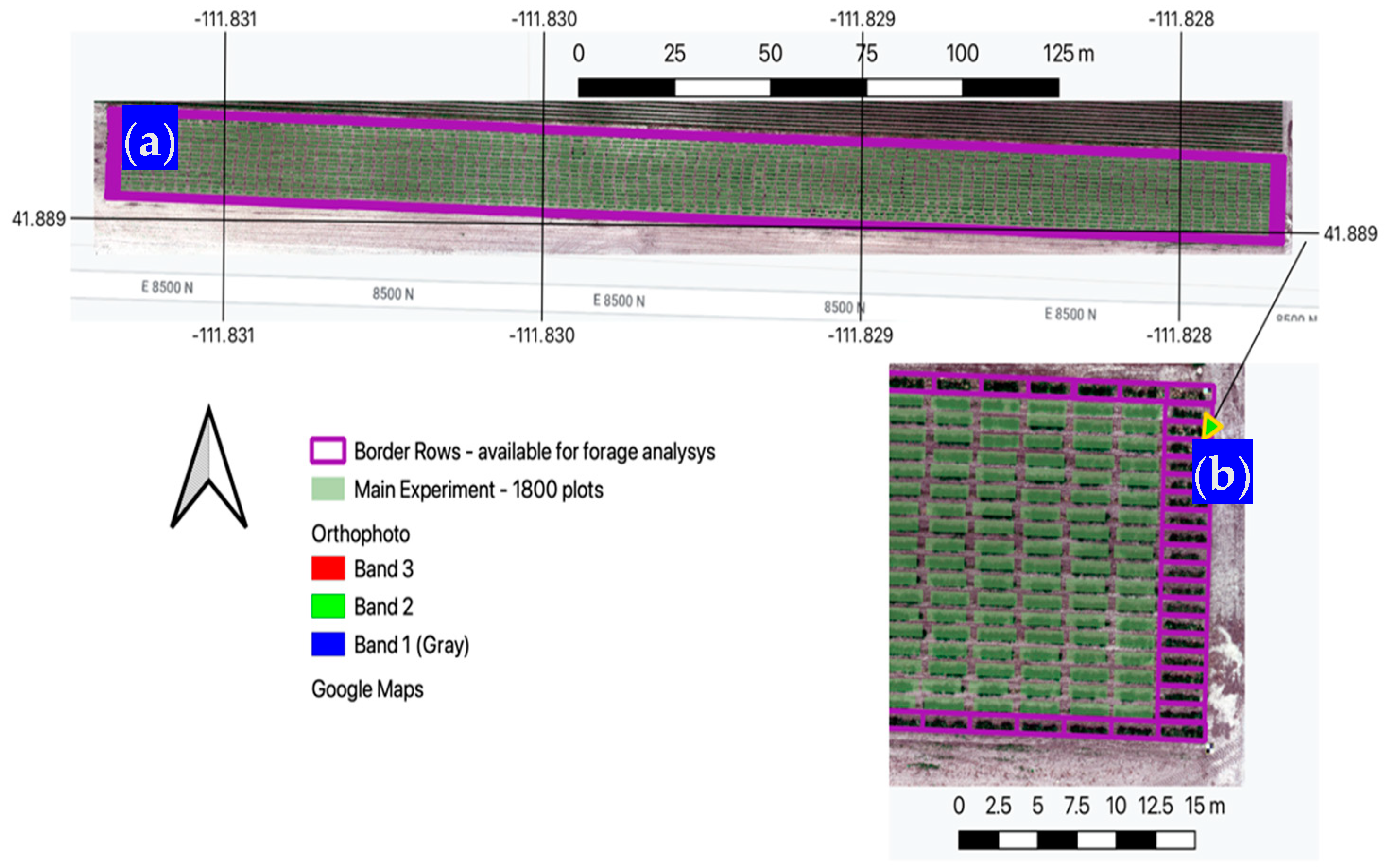
The Utah State University (USU) Richmond research farm is roughly 2.5 km southwest of the city of Richmond and 4 km north of the city of Smithfield, Utah. The research site sits at 1375 m.a.s.l. This is a dry-summer humid continental climate with an annual precipitation of 515 mm and a mean annual temperature of 8.5 °C. A large intermediate wheatgrass (IWG) (Thinopyrum intermedium) genetic experiment was established in 2020 with the main goal of assessing traits for the selection of individuals that provide higher grain yield. The experiment per se contains 1800 individual rectangular plots (approximately 3 × 0.9 m plots arranged over 18 rows of 100 plots each) whose grain is harvested on a yearly basis. Surrounding the 1800 plots, there are 240 border plots that were available for this forage analysis.
The 240 border plots were assigned a unique identifier. The unique identifier allowed the random selection of ten (10) plots for each harvest date. Harvest data were acquired on the following dates: May 05, 12, 19, 23, 31; June 06, 16, and July 05 and 19 of the year 2023. By randomizing the selection of border plots, we attempted to capture as much spatial variability of forage yield from this experiment as possible. Furthermore, because the harvests were conducted during the span of two and a half months, we were able to sample different growth stages of IWG. Border plots at Richmond (Figure 3) were harvested using a gas-powered grass trimmer, and the green matter was then placed inside plastic tote containers (Figure S1 Supplementary Material). The total weight (kg) was recorded at the field (with and without a tote). A representative sample from each plot was bagged, weighed, and then taken to the lab to be dried to determine dry matter weight.
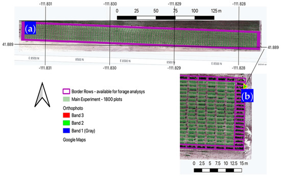
Figure 3.
(a) General location of the IWG main experiment and border plots; (b) Closer look at the far eastern section showing individual border plots as they were used in this study. Arrow points to zoomed in area.
2.2.3. Millville Farm—Sparse Canopy Grass
Bluebunch wheatgrass (BBWG) (Pseudoroegneria spicata) forage samples were collected at the USU Millville, UT research farm. The elevation at this site is 1433 m.a.s.l. It has a warm-summer continental climate with an annual precipitation of 419 mm and a mean annual temperature of 8.2 °C. The BBWG experiment was established in the fall of 2021 and consisted of 2236 rectangular plots with dimensions of 2 × 0.25 m (Figure 4). Forage harvests were conducted during the first (2022) and second year (2023) of establishment. During the first year of sampling, we collected 111 plots (~5%), and in the second year, 214 plots (~10%). For every year of sampling, we randomized the locations of the plots to be harvested to capture enough spatial variation across the field.
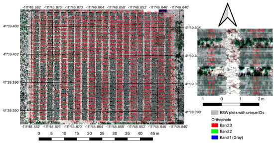
Figure 4.
General location of the Bluebunch wheatgrass (BBWG) main experiment with inset showing more detail of individual plots. Arrow indicates North.
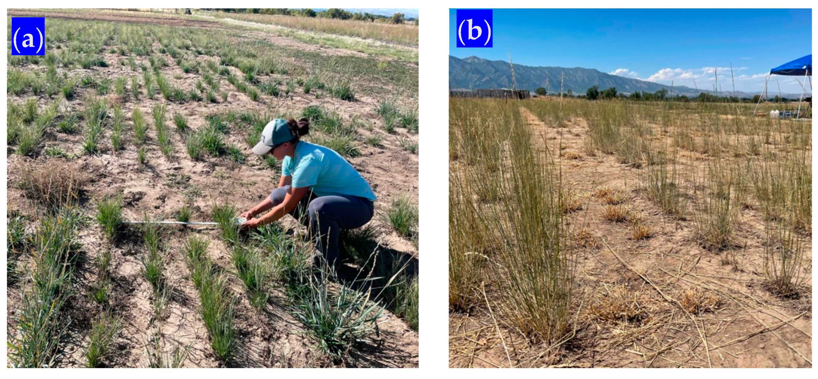
The total weight (kg) of green matter was recorded at the field, and subsequently taken to the laboratory to be air-dried and weighed. Bluebunch wheatgrass plants for each plot were manually harvested using grass clippers (Figure 5). We must report that there was significant herbivory damage to the BBWG plant canopies during the year 2023 due to chewing insects, namely grasshoppers. Examples of defoliation in this site can be seen in the Supplementary Materials (Figure S2).

Figure 5.
(a) Harvest activities during the 2022 sampling season; (b) recently harvested plots in 2023. Grasshopper damage can be observed in the surrounding plants.
Plot boundaries for all three sites in this study were obtained by manually digitizing over high-resolutions recent (2022) orthophotomaps, and in the case of Millville, the boundaries were verified using Emlid Reach-2 global positioning systems GPS rover devices with an average root mean square (RMS) error of ±2.0 cm.
2.3. RGB and Multispectral Data
2.3.1. Field Data Collection
We acquired very high spatial resolution imagery over each of the three sites using unmanned aerial vehicles (UAVs) prior to each forage harvest. We utilized a Matrice 600 Pro hexacopter, carrying a Micasense Altum-PT multispectral sensor onboard. The Altum-PT collects co-registered spectral information on the red, green, and blue (RGB) spectrum, as well as the red edge and near-infrared (NIR) parts of the electromagnetic spectrum. UAV flights were prepared using the professional drone mission planning software UgCS version 4.17. All missions were collected at an altitude of 34.8 m, which resulted in a ground spatial distance (GSD) of 1.5 cm (i.e., pixel size).
For all missions, sidelap (the distance between flight lines) and frontlap (the distance between successive photos inside each flight line) were configured to yield a minimum of 75% overlap. UgCS missions (Figure 6) were prepared so that the UAV would be able to follow the variations in the terrain and, thus, maintain a constant elevation above the ground. Before each harvest was scheduled, the weather forecast was followed carefully to avoid cloudy or rainy days. All missions were conducted during sunny or lightly overcast days and only during a particular window of time of two hours before and after local solar noon.
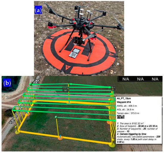
Figure 6.
(a) The Matrice 600 UAV used with the calibration panel. (b) A UgCS snapshot for the flight mission in Shandon, California.
Immediately before and after each flight mission, we took images of the Micasense sensor-calibrated reflectance panel. This is fundamental during post-processing in order to generate surface reflectance [21] products. The Micasense sensor was placed onboard the aircraft in such a way that was always pointing straight down or as close to the nadir (perpendicular to the ground) as possible. All missions were flown using a lawn-mowing pattern from east to west and vice versa. Terrain relief at all sites was flat, and thus, there was no need to account for slope effects during the flights. An average of six to ten ground control points (GCPs) were laid out on the corners and center areas of each experiment. The location (latitude and longitude) and altitude of each GCP were collected using the Emlid Reach-2.
2.3.2. Post-Processing of Aerial Imagery
We used the Micasense image processing scripts [22] to convert the raw digital numbers of the images to radiance and then to actual surface reflectance. Images were then processed using the photogrammetry platform WebODM [23]. Within WebODM, the imagery was first aligned and rectified to real-world coordinates using the collected GCPs. Subsequently, a georeferenced digital surface model (DSM)—a three-dimensional representation of the surface—and fully stitched orthorectified spectral (RGB, red edge, NIR) mosaics were extracted for each single flight mission at each study site prior to each forage harvest. All the raster or image outputs were generated in TIFF format files.
2.3.3. Derivation of Vegetation Indices: RGB and Multispectral
We developed computational workflows in the R scientific language [24] to generate vegetation indices (VIs) [25] of interest for the modeling of our variable of interest: forage yield. VIs are spectral transformations of the original RGB, red edge, and NIR bands that are generated to highlight the contribution of vegetation in comparison to other land features (rocks, soil, water, etc.) and allow spatiotemporal comparisons of photosynthetic activity and canopy variations between different types of vegetations [26]. This is particularly useful in our analysis to compare variations between the forage grasses of interest. We used the R package FIELDimageR [27] to generate VIs that are exclusive to the RGB part of the electromagnetic spectrum and also VIs that require the extra red edge and NIR spectral bands (Table 2). The formulae for the different indices can be found in [25,27].

Table 2.
Vegetation indices—RGB and multispectral—used in this study.
All these vegetation indices were calculated at the pixel level (GSD of 1.5 cm), and thus, covered the same spatial domain as the DSM and orthophotos extracted using the WebODM photogrammetry software (https://www.opendronemap.org/webodm/).
2.3.4. Extraction of Representative Values per Plot: Zonal Statistics
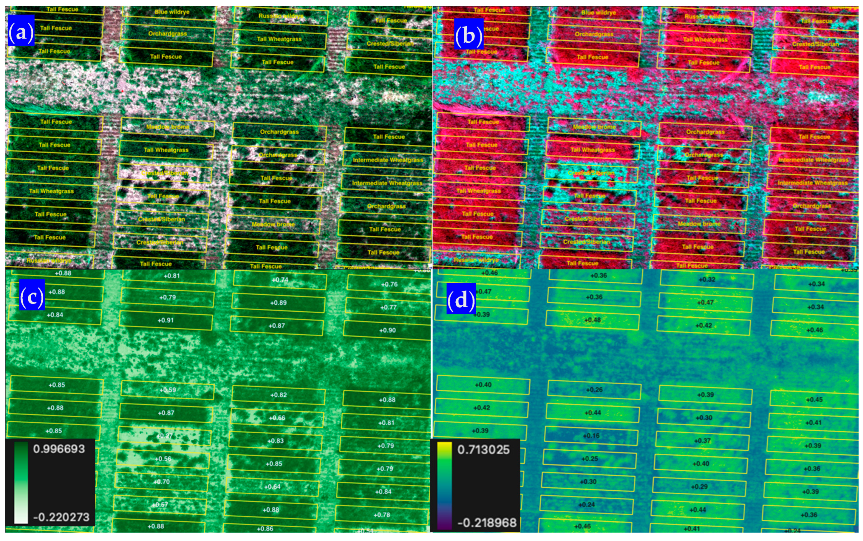
The polygons that correspond to each field plot in this analysis can contain thousands (Millville~2223) to tens of thousands (Shandon~22,223) of cells or pixels for each image or raster file. Recall that each pixel was 1.5 cm or 0.000225 m2. A sample of the imagery for the plots at the Shandon site can be seen in the next figure (Figure 7). In this figure, different imagery representations are provided (i.e., natural color and false color). For the same spatial subset, we provide two vegetation indices: the normalized difference vegetation index and the normalized difference red edge index. This helps to depict how each plot’s feature (fully covered by grass or vice versa) can impact the values of the resulting vegetation indices (Figure 7).
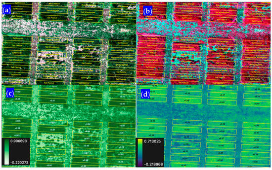
Figure 7.
Subset of imagery for the Shandon, CA, site in (a) natural color (RGB), (b) NIR red and green false colors, (c) the normalized difference vegetation index (NDVI), and (d) the normalized difference red edge index (NDRE).
To use the raster information in a modeling scheme, we needed to summarize it for each plot. We computed zonal statistics using the R package exactextractr [28], which has the advantage over other zonal statistics algorithms that accounts for pixels that are fully or partially contained within each plot polygon. The exactextractr package is written in C++ language and can provide summarizations faster than other R packages.
The zonal statistic used in this research is the median, as this value is not affected by extreme outliers for land features (i.e., bare ground, rocks) that may be present in each plot. Median values for the individual spectral bands (red, green, blue, red edge, and NIR) and the generated vegetation indices were calculated for each plot polygon for each available UAV flight.
2.4. Statistical Modeling
2.4.1. The Response and Independent Variables
We designated the response variable as forage yield (kg ha−1), which we computed for each individual plot by dividing the total plot weight (kg) recorded at the field (i.e., mechanic harvester, grass clippers) by the area of the plot in hectares. Because plots of three different sizes were used in this analysis, we needed to normalize the forage wet weights measured at the field across the three research sites into one cohesive variable. The denominators used were (a) 0.00027 ha for Richmond (plot dimensions 3 × 0.9 m = 2.7 m2), (b) 0.0005 ha for Shandon (plot dimensions 5 × 1 m = 5 m2), and (c) 0.00005 ha for Millville (plot dimensions 2 × 0.25 m = 0.5 m2).
Our predictor variables were the median values extracted for the spectral bands, and derived vegetation indices. In addition, we included the volumetric or 3D space that the grasses project from the soil to their canopy at each plot (Figure 8). We extracted this volume from the digital surface model as follows:
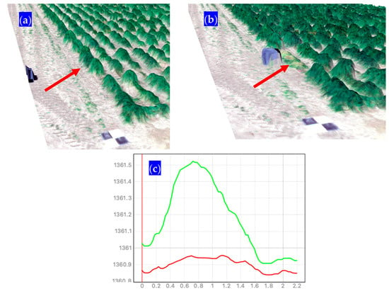
Figure 8.
Sample of a typical DSM collected at the Richmond, UT site with (a) a border plot of IWG selected for forage harvest; (b) the same plot was collected and green matter placed inside tote; and (c) typical grass canopy height (green line) and ground level (red line) used for the volumetric 3D space calculation. Arrows point to the same plot pre and post-harvest.
- We intersected the polygon boundaries for each plot with the DSM;
- The upper level (canopy height per se) equaled the proper DSM values in m.a.s.l.;
- The base level (ground height) was computed as the average elevation (m.a.s.l.) of the plot polygon vertices that intersected the DSM;
- The height profile differences (grass canopy height—ground level height) were extracted at the pixel level;
- A simple volume cut/fill calculation was conducted whereby height differences were multiplied by the area (0.000225 m2) and summed over all pixels within the plot’s polygon.
The volumetric 3D space was added to the median values obtained previously (Section 2.3.4). A modeling matrix was built for each site where rows contain individual observations (plots), and the columns are (a) the response variable to forage yield in kg ha−1 and (b) predictors or independent variables, such as spectral data, vegetation indices, and the volumetric 3D space.
2.4.2. Model Fit—Stratified Cross-Validation (SCV)
Our main goal was to develop a global model that was able to make reasonable predictions across sites, across grass species, and across the different stages of growth of our continuous variable forage yield. In this case, we used a regression model. We chose to evaluate the performance of basic linear regression, as well as a non-parametric modeling approach using random forest [29] regression via a k-fold cross-validation routine. Although the response variable forage yield was standardized, there were a few situations that needed to be dealt with before attempting to find an appropriate model fit:
- Species with dense (i.e., Richmond IWG, and all the grass species at Shandon) and sparse (BBWG at Millville) canopies were included.
- There were three research sites.
- Harvests were conducted multiple times to include variability in plant growth stages.
In light of these situations, we chose to conduct a stratified cross-validation SCV [30] scheme where each of the strata would be left out at each iteration for model validation while the rest of the strata are used for model fit. We believe that such a strategy equalizes opportunities for sites, species, and stages of growth to fully participate in the final model’s fit. We organized the strata by concatenating the site, harvest at each site, and species into an additional attribute in the database (Table 3). Only species with a number (n) equal to or higher than 50 observations were used in the training of the model. Species with n < 50 were used as another set of validation for the developed models. The following sample sizes were available for those species directly used in model training: 61 for orchard grass (Dactylis glomerata), 138 for intermediate wheatgrass IWG (Thinopyrum intermedium), 325 for bluebunch wheatgrass BBWG (Pseudoroegneria spicata), and 457 for tall fescue (Festuca arundinacea).

Table 3.
Sample preparation of the strata to be used during K-fold cross-validation model fit.
The resulting stratum was added to each observation (plot) in the modeling matrix in an additional column containing this string or concatenation of text. This attribute could then be used as a factor for assigning one stratum to each observation.
2.4.3. Fitting and Validating Models for RGB and Multispectral Imagery
We utilized a stratified k-fold cross-validation strategy to find the “best” model in terms of a model structure that balances performance by minimizing the root mean square error RMSE, R2, and mean absolute error MAE. We conducted this process in the following five independent ways:
- A.
- A simple ordinary least square linear OLS regression model used only volumetric 3D space as a predictor. Hereafter, it is referred to as LM-3D.
- B.
- Multiple linear regression models used volumetric 3D space, RGB bands, and related Vis, hereafter referred to as LM-RGB.
- C.
- Multiple linear regression models included using volumetric 3D space, RGB bands and related VIs in addition to the red edge, NIR bands, and related VIs. Hereafter, it is referred to as LM-Multi.
- D.
- The random forest regression model used volumetric 3D space, RGB bands, and related VIs (Table 2), hereafter referred to as RF-RGB.
- E.
- A full random forest model, in addition to volumetric 3D space and RGB spectrum, also included red edge, NIR, and related Vis., hereafter referred to as RF-Multi.
Except for (A) above, the process to select the predictors for use in each one of the model variants was the following:
- (a)
- Fit temporary random forest models with all their available predictors for a particular model variant, as explained above. For instance, for variant (B) above, a temporary random forest model with volumetric 3D space, the three RGB bands, and all the RGB indices (i.e., BI, SCI, GLI, NGRDI, VARI, BGI) were fitted.
- (b)
- For each of these temporary random forest models, we extracted information of variable importance [31,32] to identify the most relevant features or predictor covariates for prediction. At the same time, the variable importance rankings allowed us to filter out low-importance or irrelevant variables to enhance model performance.
- (c)
- From the variable importance plots, we used the mean decrease in predictive accuracy to select the predictors that would participate in each model variant. While there was no consensus [33] in the literature about what threshold to use to select the major predictors, we arbitrarily chose to keep the predictors with the highest scores (>35% in importance).
Five major steps were followed and coded in an R programmatic routine:
- Divide the entire modeling matrix into two sets: (a) one for a model fit with 75% of the observations and (b) the rest of the observations for independent validation. This second set is a completely independent set that was never used during the cross-validation process. We used the splitTools R package [34] with the Species-Site-Harvest strata (Table 3) as an attribute to guarantee that each set (training and validation) would include observations from all available strata.
- We used the R package caret [35] “groupKFold” function to split the data based on groups—using the Species-Site-Harvest attribute. Using this function makes sure one of the groups is not contained in the training and is left out for validation.
- The output object from “groupkFold” was used in caret’s “trainControl” function as an index. This index is the observations (plots) unique identifier in the modeling matrix, and it is used to tell the algorithm which observations are used during each k-fold iteration. In the “trainControl” function, we specified the method to be “cv” or cross-validation.
- We used the train function of the caret package to iteratively run all the k-fold cross-validations and select a model that minimizes the error, as stated earlier. The method selected in this function was “LM” for simple/multiple linear regression and “RF” for random forest regression, the response variable was the forage yield in kg ha−1, and the predictor’s volumetric 3D space, individual spectral bands, and vegetation indices.
- The previous steps were repeated for the simple model LM-3D, the reduced RGB models (LM-RGB and RF-RGB), and the full multispectral models (LM-Multi and RF-Multi). Recall that in the simple LM-3D model, we only included the volumetric 3D space, while in the reduced RGB models, we only included the red, green, and blue RGB bands, associated Vis, and the volumetric 3D space. The full models included all available predictors.
2.4.4. Comparison of the Global Models
The general performance of our SCV global models (LM-3D, LM-RGB, LM-Multi, RF-RGB, and RF-Multi) was assessed using traditional regression metrics, such as RMSE and MAE. In addition, we calculated scores for the Regression Receiver Operating Characteristic (RROC), as proposed by [36] and implemented in the R package auditor [37]. Due to the nature of the SCV models, where each grass species was left out at each iteration, extraction of the RROC on a per-species basis was not feasible, and thus, we conducted the RROC calculation for each global model.
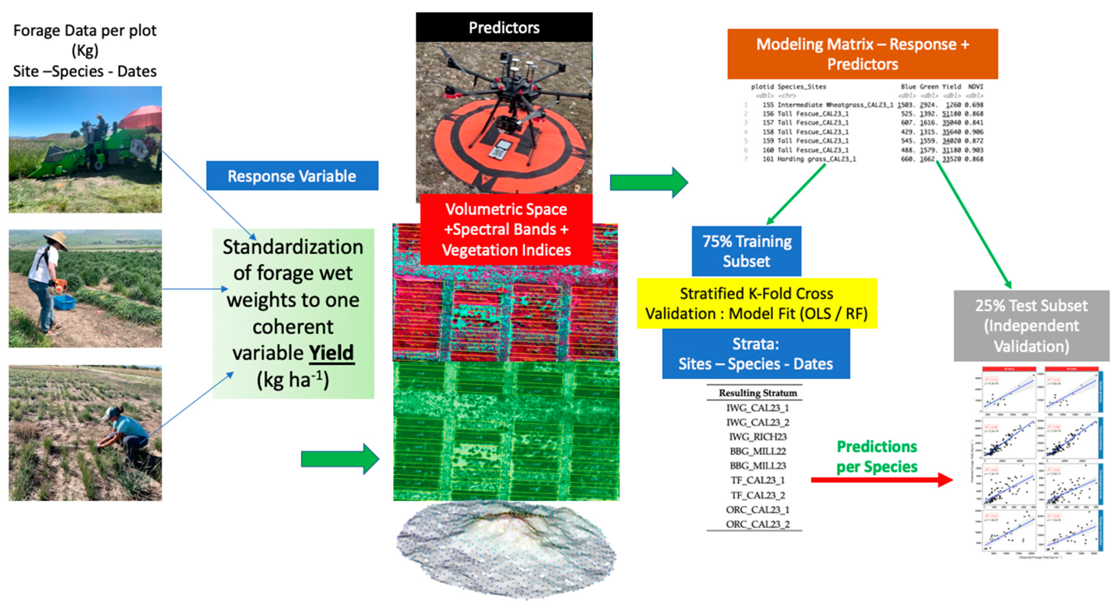
The following schematic (Figure 9) graphically summarizes the Methods section for our research.
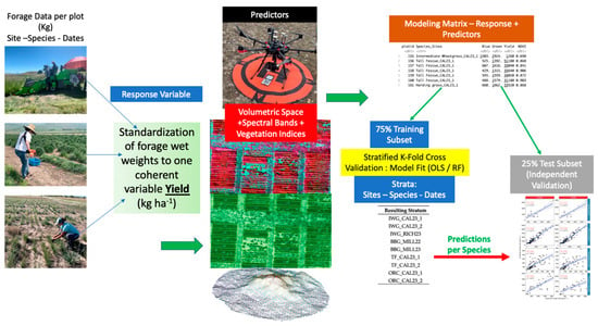
Figure 9.
Graphic summary of the methodology used in this study.
3. Results
3.1. Field Harvest Wet Weights Are a Reasonable Representation of Forage Yield
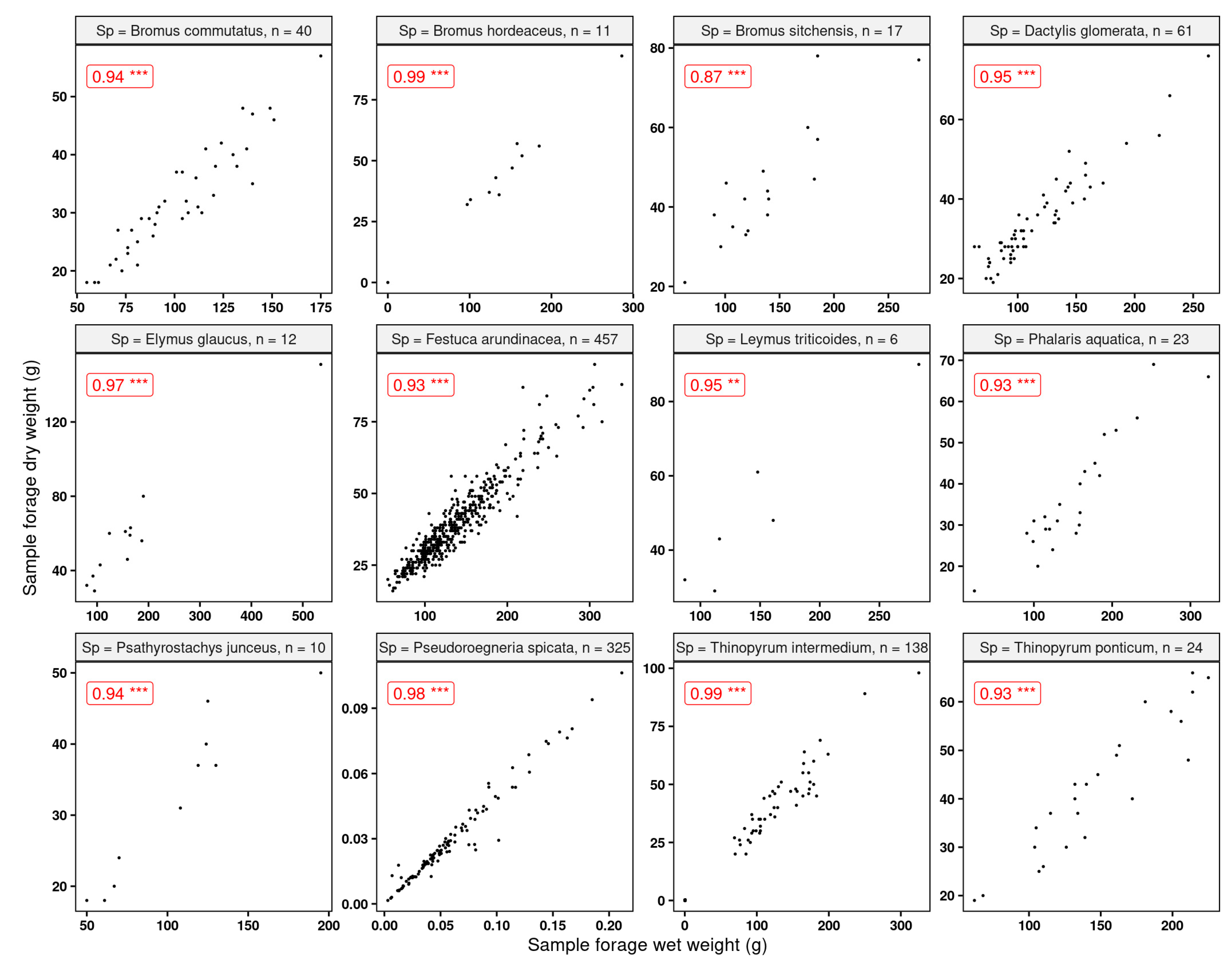
Apart from Bromus sitchensis, we found very good relationships (R > 0.75) between the sample wet and dry weights (Figure 10). This is an indication that modeling the wet weights—or, in our case, the standardized variable forage yield—to make inferences is a reasonable approach.
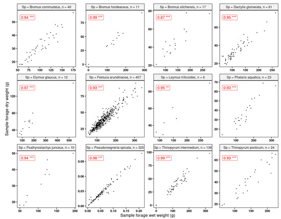
Figure 10.
Correlations between sample wet and dry weights for the grasses used in this study. All correlations were significant at p-value 0.05. “n” indicates the number of observations. Statistical significance: ** p ≤ 0.01, *** p ≤ 0.001.
In addition, collecting the per-plot grass samples provided us with a clear idea of the plant water content variation between species. As can be seen (Table 4), the range of the percentage of moisture content is almost 20%, with a global average of 70.1%. Among the studied species, Elymus glaucus Buckley (blue wildrye) showed the lowest plant moisture content, while Pseudoroegneria spicata (bluebunch wheatgrass) had the highest. Plant moisture content was calculated by dividing the difference between wet and dry weights by the wet weights.

Table 4.
Mean sample wet and dry weights with calculated plant moisture content for the grasses used in this study.
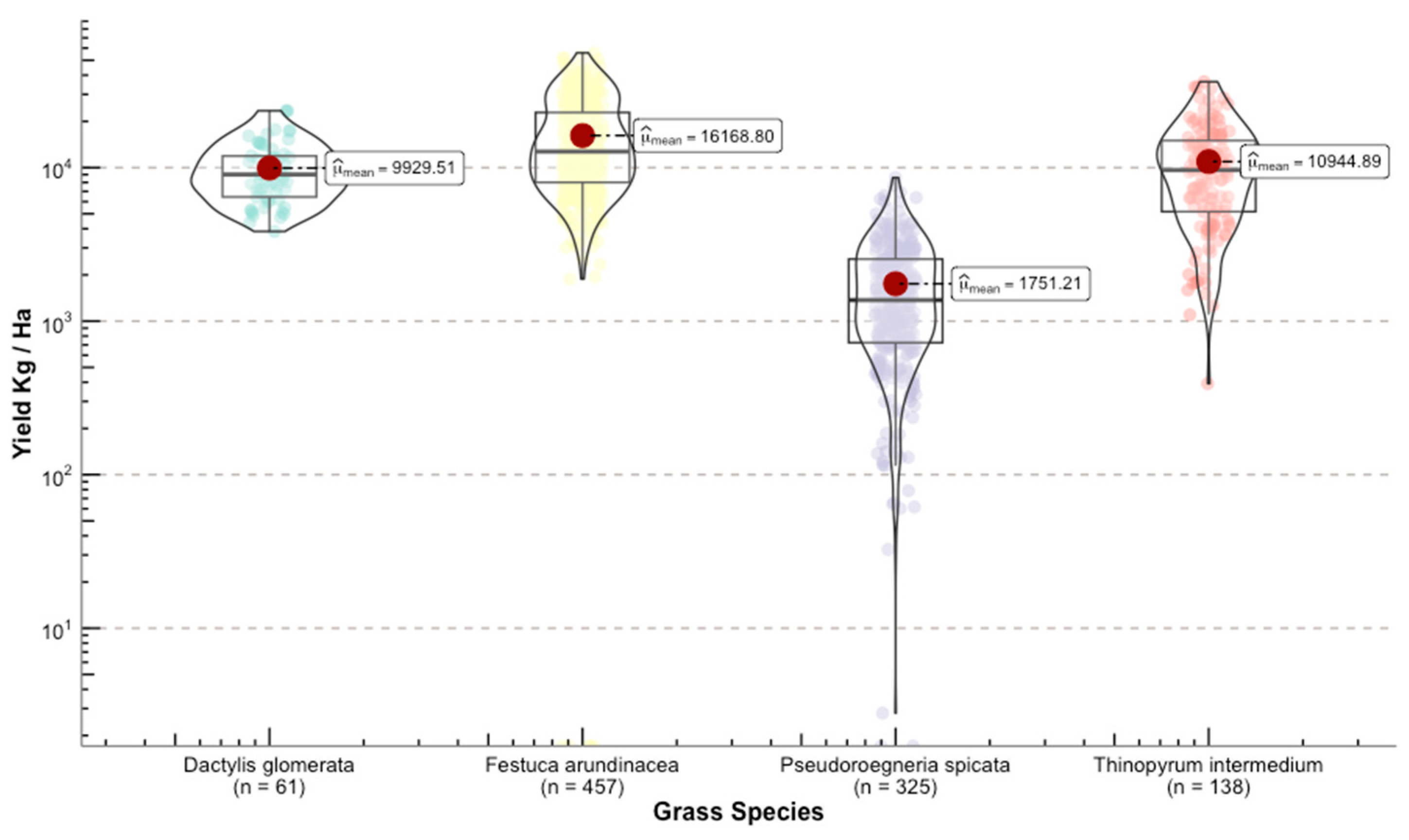
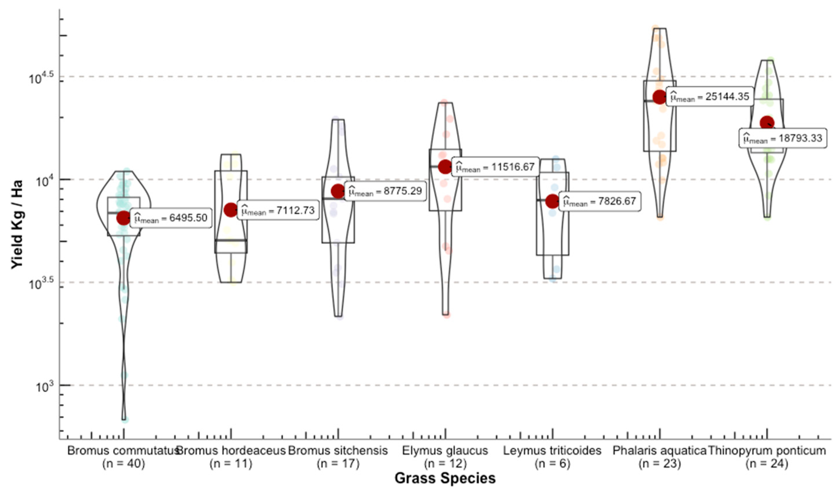
Once we converted the per-plot wet weights to forage yields (kg ha−1), we were able to see the differences in yield among grass species (Figure 11). The range for the calculated means of the standardized variable was 23,393 kg ha−1 between the highest yield Phalaris aquatica L. (bulbous canarygrass) and the lowest Pseudoroegneria spicata (bluebunch wheatgrass BBWG).
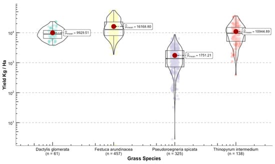
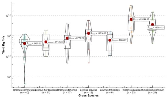
Figure 11.
Distribution of the response variable forage yield between the selected grasses for this study. Upper panel shows the species used for model building. Lower panel depicts grasses that were used for independent validation.
3.2. Photogrammetry-Derived Volumetric 3D Space
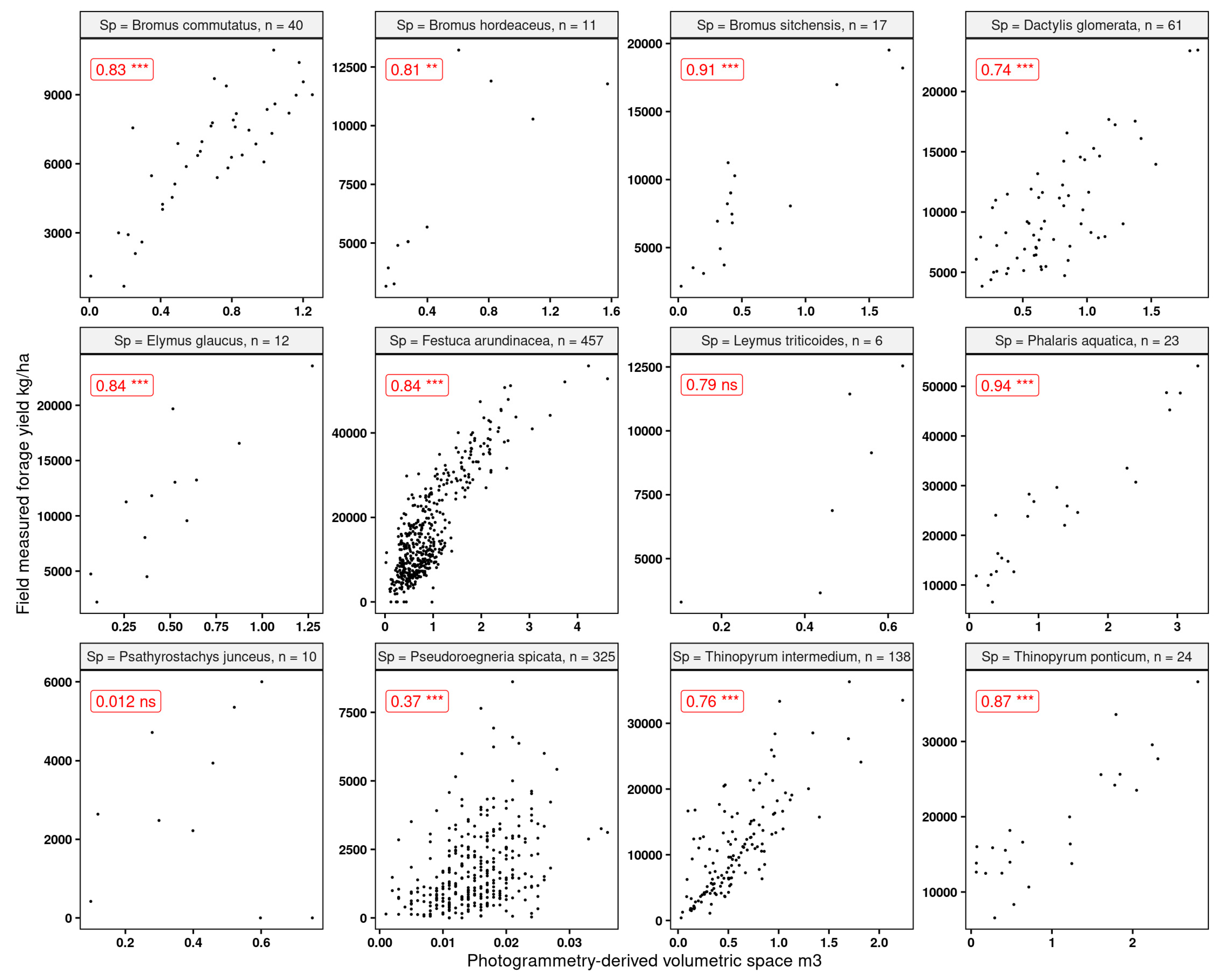
Since one of the main goals of this research was to explore the feasibility of using RGB-based systems, we explored the strength of the relationship between volumetric 3D space (Section 2.4.1) and the forage yield. We expected to find stronger relationships for the denser canopy grasses as opposed to the sparse canopies (i.e., P. spicata). We found (Figure 12) that the strongest linear relationships (R2 > 0.8) were found for Phalaris aquatica and Bromus sitchensis, both of which showed a fuller canopy at the time of harvest. The poorest associations were found for the sparse canopy grasses, where it was very clear that the computed volumetric 3D space struggled to capture the acceptable fit of the measured forage yield.
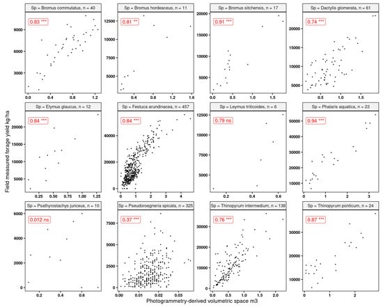
Figure 12.
Linear correlations and Spearman significance between the computed volumetric 3D space and forage yield for the grasses used in this research. “ns” indicates that the correlation was not significant, and the rest were significant at p-values 0.05. “n” indicates the number of observations. Statistical significance: ** p ≤ 0.01, *** p ≤ 0.001.
While these results did not provide much promise for the sparse canopy grasses, they were encouraging for the majority of the dense canopy species. The volumetric 3D space is a relatively straightforward variable to model forage yield. This is quite important since it is a variable that can be generated from either simple RGB sensors or from more complex high-end multispectral sensors. While the volumetric 3D space was not a strong linear predictor for sparse canopies, the rest of the covariates (spectral bands and derived vegetation indices) showed a relatively strong (R2 > 0.7) association with the response variable of forage yield.
3.3. Model Outputs
3.3.1. Chosen Predictor Variables
With the application of the rule that we set up (Section 2.4.3) of only selecting predictors with an importance of 20% or higher, the following covariates were selected:
- We selected five (5) variables for model variants B (LM-RGB) and D (RF-RGB). These were (in order of importance) as follows: volumetric 3D, BI, GLI, SCI, and BGI.
- For model variants C (LM-Multi) and E (RF-Multi), we selected eight (8) predictor variables. These were (in order of importance) as follows: volumetric 3D, GNDVI, RVI, NDVI, NDRE, GLI, BI, and BGI.
We provide variable importance plots for the model variants in the Supplementary Materials (Figure S3).
3.3.2. Linear Regression Models—Validation Dataset
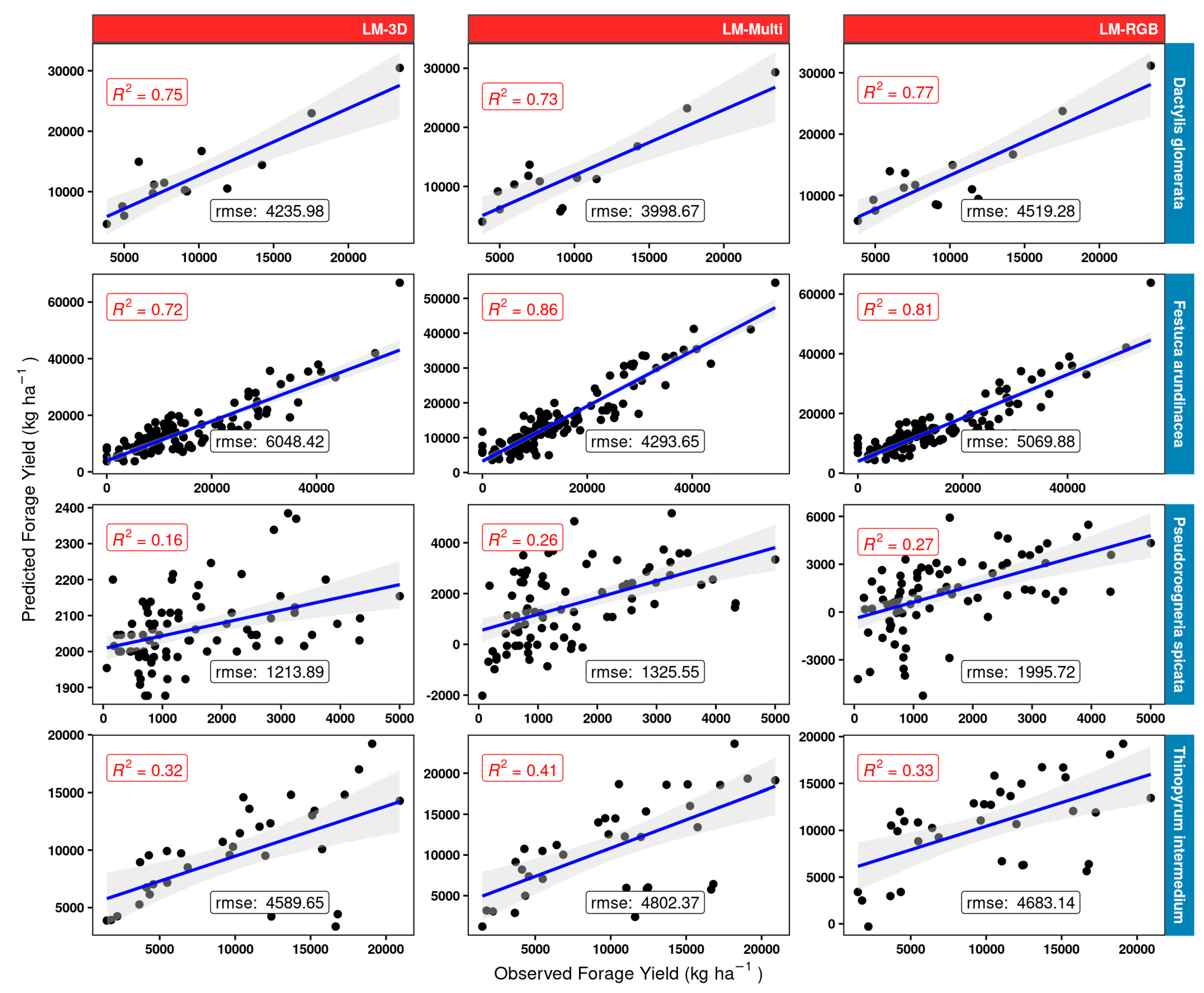
Results (Figure 13) suggest that using only the volumetric 3D space in a very simple linear regression model may be quite sufficient for orchard grass (D. glomerata), as the R2 obtained did not show much variation between the simple model LM-3D and the LM-RGB or multispectral LM-Multi models (R2 in the mid 0.70 s). There was considerable gain, however, between using the LM-3D model and the LM-RGB or LM-Multi model for tall fescue (F. arundinacea). The results show that using RGB + derivatives (LM-RGB) increases the R2 by 0.09 units compared to the simple LM-3D model. The increment in this value increases up to 0.14 when using the entire array of multispectral bands and vegetation indices (LM-Multi). Poor results were obtained for the mostly sparse canopy grass bluebunch wheatgrass (P. spicata) as the best R2 using linear models was 0.27 (LM-RGB model). Here, the LM-RGB was nearly as good as using the full multispectral model (LM-Multi). The best model for IWG (T. intermedium) was the multispectral LM-Multi and gave moderate accuracy (R2 = 0.41). Using the simple LM-3D model or the LM-RGB gave fundamentally the same results (R2 in the low 0.3 s) for IWG.
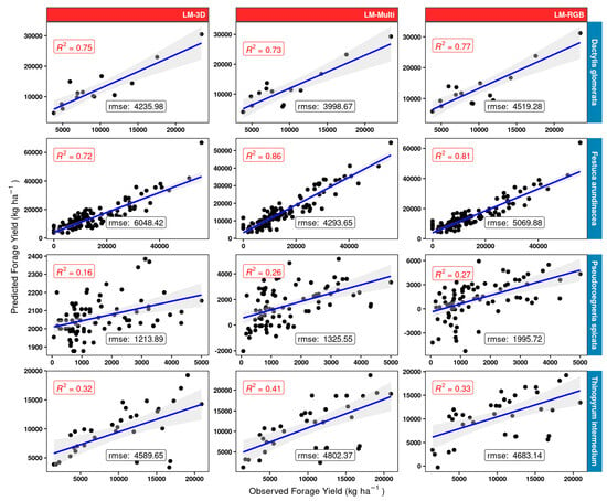
Figure 13.
Linear models LM-3D, LM-RGB, and LM-Multi scatterplots and measures of performance (adjusted R2 and RMSE) for the different model structures (red panels) using the 25% validation subset for four grass species (blue rows) used in model building. “rmse” is given in kg ha −1 units.
3.3.3. Random Forest Regression Models—Validation Dataset
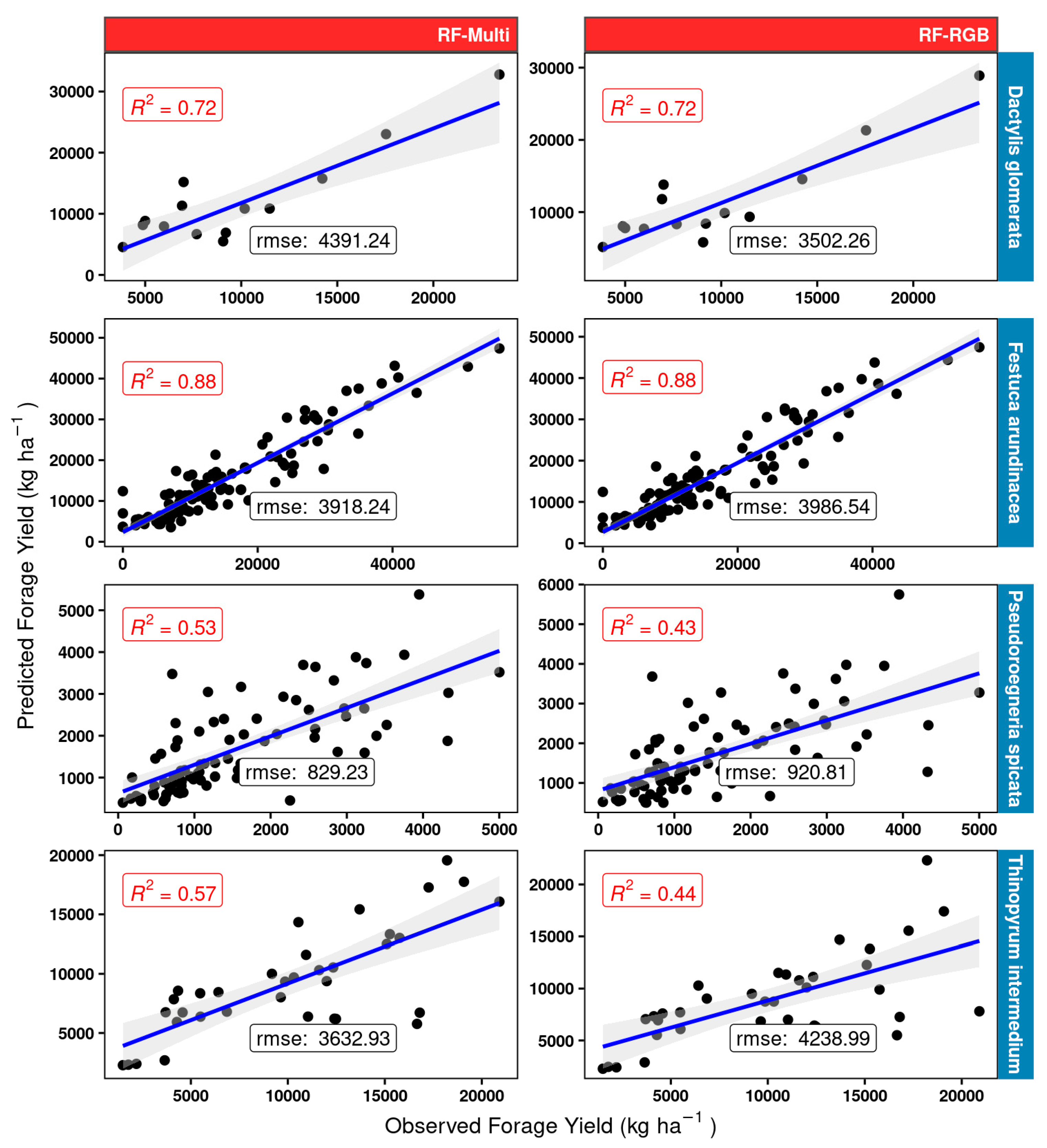
About the RF model fit (Figure 14), the results were very similar to those shown for the linear models (Figure 13) for tall fescue and orchard grass. Considerable gains with respect to the linear model fit were obtained, particularly for bluebunch wheatgrass, however. The best RF model was the one using the multispectral dataset (RF-Multi), which provided a two-fold improvement in accuracy (RF-Multi R2 of 0.53 compared to R2 0.26 for the LM-Multi) for this grass. Furthermore, using the multispectral data resulted in a gain of 0.13 R2 compared to using the RF-RGB model. While not as prominent as the gains observed for BBWG, the RF model using the multispectral data RF-Multi for intermediate wheatgrass IWG resulted in an R2 of 0.57, which is much better than the best linear LM-Multi model (R2 of 0.41).

Figure 14.
Random forest RF model scatterplots and measures of performance (adjusted R2 and RMSE) for the different model structures (red panels) using the 25% validation subset for four grass species (blue rows) used in model building. “rmse” is given in kg ha −1 units.
3.3.4. Regression Models—Exploration of Defoliation Effects
Given the severe defoliation by grasshoppers observed (Figure 5b and Figure S2) at the Millville, UT site for the year 2023, we hypothesized that this was a major element in the poor performance of the simpler models (i.e., LM-3D, LM-RGB, LM-Multi—Figure 13). We explored this effect by fitting a different model structure, where we completely excluded the stratum corresponding to Millville BBWG 2023 while keeping the rest of the strata intact. Coefficients of determination are presented in the next table (Table 5) for this variation in the overall model structure. While quite positive effects are evident for intermediate wheatgrass IWG (highest R2 being 0.65 compared to 0.57—Figure 14) and for bluebunch wheatgrass BBWG (highest R2 being 0.76 compared to 0.53—Figure 14), overall, there were neither negative nor positive effects for tall fescue. The results for orchard grass (D. glomerata) are detrimental; however, regarding the linear models. The highest R2 was obtained using LM-Multi at 0.6 compared to values in the ~0.75 range (Figure 13) for this species. The highest value for this grass was 0.63 using the random forest model with the multispectral datasets RF-Multi.

Table 5.
Coefficients of determination for the different model structures (Linear and RF) using the 25% validation data where the BBWG 2023 stratum was excluded. Bold and underlined entries identify the best model (highest R2).
3.3.5. OLS and Random Forest Regression Models—Unused Grasses
We present (Table 6) the adjusted R2 for the grasses (n < 50) that were left out as a completely independent dataset. Scatter plots can be found in the Supplementary Material (Figures S4 and S5). Based on the coefficients of determination alone, it is shown that the simple LM-3D model structure (linear model with the volumetric 3D space as lone predictor) provides the best fits for three (tall wheatgrass (T. ponticum), meadow brome (B. commutatus), and Alaska brome (B. sitchensis)) out of the seven grasses. While the best model for harding grass (P. aquatica) turned out to be the LM-Multi multispectral, this resulted in a difference of only 0.03 R2 units compared to the simple LM-3D model. Much greater differences were found for brome grass (B. hordeaceus), beardless wildrye (L. triticoides), and blue wildrye (E. glaucus), where it was very clear that using a multispectral dataset LM-Multi provides a significant gain over the LM-RGB or just the volumetric 3D space LM-3D.

Table 6.
Coefficients of determination for the different model structures (Linear and RF) for the grass species that were not used during model building. Bold and underlined entries identify the best model (highest R2).
3.3.6. Global Models’ Performance
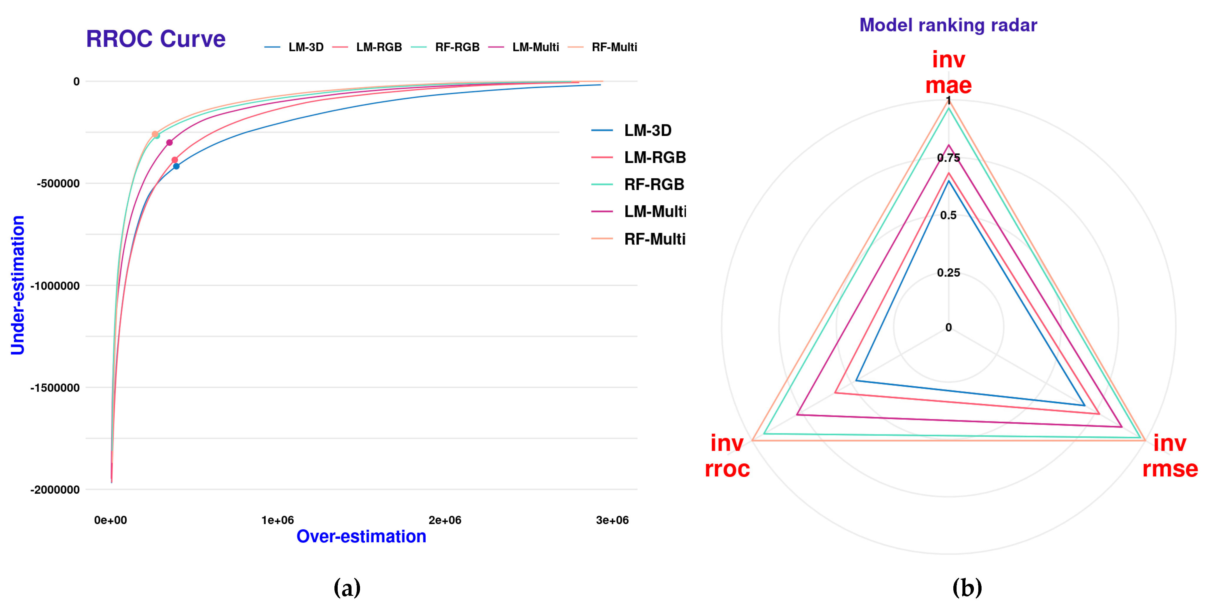
The RROC curves for the different regression models are shown (Figure 15a). This plot shows for each model the magnitude of overestimation (x-axis) and underestimation (y-axis) as defined by [36]. The base of the plot is a shift, which is equivalent to the threshold for traditional ROC curves. The point where the shift equals 0 is represented by a dot. Shifts that are closer to the 0,0 origin (upper-left corner of the plot) are indicative of an overall better model performance. In Figure 15a, we can see that there is a gradual trend in model improvement in the incremental order: LM-3D, LM-RGB, LM-Multi, RF-RGB, and LM-Multi. This trend corresponds quite well with the performances shown for each species in Figure 13 and Figure 14. In addition, we present the scaled (values 0 to 1) scores for the performance metrics (RMSE, MAE, and RROC) in a model ranking radar plot (Figure 15b). In this plot, values closer to one (one) indicate an overall better model performance. It becomes more evident that the non-parametric models (RF-RGB and RF-Multi) outperform the linear regression models in all three calculated metrics.
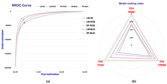
Figure 15.
RROC curves with magnitudes of over and under estimations in predicted values (a) and scaled (0–1) regression performance metrics (b) for the five global SCV models.
4. Discussion
4.1. On the Use of Wet Weights Instead of Dry Weights
Research has shown that using dry weights is more fitting to model forage yield than wet weights due to various reasons that deal with accuracy, reliability, and consistency. Wet weights include the weight of the water in the forage, and these can vary widely depending on the moisture content and environmental conditions. Conversely, dry weights represent the actual mass of the organic matter in the forage and, thus, make it a more direct measure for estimating biomass [38]. Regarding nutrient content, dry weights are a better indicator of forage quality, which is assessed based on the concentration of nutrients, and these are present in higher concentrations in the dry matter of the forage. Therefore, using dry weight allows for a more accurate assessment of the nutritional value of the forage [39]. Furthermore, dry weights are more suitable for comparing forage biomass across different studies or locations because wet weights can be influenced by environmental factors, such as moisture content [40]. In our modeling, there is a fundamental reason to utilize the wet weights. The spectral information that the digital sensors (i.e., RGB, multispectral) captured at the fields is a direct reflection of the grasses’ green matter, which includes the water content at the time of each flight. While there are exceptionally high correlations between wet weights and dry weights for our samples (Figure 10), we did not want to conduct an indirect regression using the dry weights as the response variable since the spectral data and derivatives (i.e., NDVI, NDRE) collected over the green matter plots. Furthermore, using dry weights carries the complexity that samples must be transported and dried in specialized facilities. Drying the full contents of 5 m × 1 m plots (i.e., the dimensions of the Shandon site) was neither practical nor feasible. We considered that the strong correlations between wet and dry weights for the samples support our utilization of wet weights as a transparent proxy for forage yield. Finally, the multispectral imagery provides wall-to-wall spatial coverage of each field plot, not just the bagged sample that was taken to the lab to measure dry weights, and thus, its information can only be related to the wet weights of the plot. We are confident that variability between sites and harvests was minimized by converting all the wet weights to a standardized measure; forage yield allows for more meaningful comparisons and analysis of forage biomass data. While we conducted different harvests, all the values were standardized, as described in the methods; however, our modeling results were not intended to provide additional insights about growth stages.
4.2. Using UAVs to Estimate Forage Yield for Grasses of Semiarid Environments
Our emphasis on testing the ability of reduced RGB datasets and derivatives is justified as several references jointly suggest that RGB imaging is the most commonly used method for estimating aboveground biomass (AGB) in grass systems using UAVs [41,42]. Overall, these papers suggest that RGB imaging is a simple and cost-effective method for estimating forage biomass using UAVs compared to higher-end multispectral sensors, such as the Altum-PT used in this study. While extensive information is found for modeling forage yield in prairie grassland systems, few studies have documented work on the grasses that were the focus of this research. A combination of the plant-normalized difference vegetation index (NDVI) and LiDAR measurements to estimate the biomass of a tall fescue pasture was conducted in Australia. In this study [43], they mounted a LiDAR unit on a vehicle to derive canopy height and used an active optical reflectance sensor to determine NDVI. The measurements of NDVI and pasture height were then combined to estimate biomass. There are reports that satellite imagery has been used to model forage biomass for Phalaris aquatica and Dactylis glomerata. In that study, they used satellite remote sensing and machine learning techniques to quantify the total standing dry matter (TSDM), standing green biomass, and standing dry biomass of these two species [44]. This research demonstrated the use of remote sensing technology, specifically satellite imagery, to model forage biomass. However, no UAV data collection was used, and plots were much larger (~1 ha) than the ones used in our research. We did not find direct evidence in the literature regarding the use of UAV imagery to model forage yields for BBGW or IWG. Studies about biomass partitioning leaf, stem, and inflorescence [45] have been reported for Thinopyrum intermedium, but this study was observational, and no UAV or remote sensing data were used. No references were found either for any of the Bromus spp. or Leymus triticoides (beardless wildrye) grasses. In this context, our research presents pioneer results in forage yield estimates for prominent species used in restoration efforts across the Intermountain United States.
4.3. The Volumetric Space as a Strong Predictor of Forage Yield
The use of metrics such as the 3D volume derived from UAV RGB imagery has been widely documented in modeling forage biomass. Researchers [46] have found that super high-resolution (1 cm/pixel) crop surface models can estimate the fresh and dry biomass of barley (Hordeum vulgare) with high accuracy. In another study [42], the application potential of consumer-grade UAV RGB imagery in estimating maize above-ground biomass was reported, and the results showed that plant height directly derived from UAV RGB point clouds had a high correlation with ground-truth data. A deep learning-based method using UAV-based RGB images was developed [47] to estimate the biomass yield of forage grass species (Panicum maximum Jacq.) with high accuracy in tropical areas. Research on maize [48] that maximized the volumetric space called by the authors BIOVP was found to retain the largest strength effect on biomass estimates. Our research has shown that for most of the grasses (Figure 13 and Table 6), the utilization of the volumetric 3D space as the sole predictor using simple linear models LM-3D rivals those results from more complex data structures (e.g., LM-RGB and LM-Multi) and more powerful modeling algorithms, such as random forests. This was evident for the dense canopy grasses whose wet weights had a very strong linear relationship (Figure 12) with the volumetric 3D space. For dense canopies (e.g., Phalaris aquatica), the digital surface model DSM that can be extracted from the dense point cloud could more accurately represent the 3D space occupied by the leafy material from the soil to the top of the canopy at the field (See Figure S6 on the Supplementary Material). The linear model can easily explain most of the variation in the estimated forage yield due to how well these grasses fill the space and how well this space can be represented by the DSM.
Conversely, poor results using the volumetric 3D space were obtained for sparse canopy grasses, such as bluebunch wheatgrass BBWG (Pseudoroegneria spicata). We hypothesize that two main factors affected the poor performance of the volumetric 3D space in this case. One factor is the severe herbivory attack that was present during the year 2023 (Figure 5b and Figure S2), where defoliation by grasshoppers eliminated vast quantities of green leaf matter. We observed better results for most of the grasses when a newer model structure did not include the year 2023 (Table 5). This clearly indicates the impact of the defoliation by grasshoppers on overall model performance. The second factor is the over-generalization that can occur with the dense point cloud during photogrammetry processing. We illustrate this assumption in the Supplementary Material (Figure S7). A grass such as BBWG projects multiple stems and seedheads in a panicle-shaped canopy that can be represented in the dense point cloud, although not completely due to the size of the stems, which, in most cases, are smaller than the pixel size used in our flights. Furthermore, many of the stems are not captured in the dense point cloud. This situation creates multiple empty spaces in the canopy that cannot be accurately represented in the digital surface model DSM. The density of the point cloud is simply not enough to generate an appropriate interpolation of elevations and 3D volumetric space estimations.
While strong limitations to modeling yield for grasses with sparse canopies using only the volumetric 3D space have been shown in our research, very acceptable results (Figure 14 and Table 6) were obtained for dense canopies. This is quite important as the volumetric 3D space can be estimated using dense point clouds generated from low-end RGB sensors, which are much more affordable than multispectral sensors.
4.4. Differences across Model Structures—How Multispectral Datasets Improve Model Fit
We found that by using the full array of spectral bands (RGB, red edge, and NIR) and vegetation indices, we were able to increase the accuracy of our predictions for sparse canopy grasses (i.e., BBWG). This was possible, however, only when the multispectral dataset was used with the random forest algorithm (i.e., RF-Multi model structure, Figure 14). We observed very poor relationships between the RGB VIs and our response variable (Supplementary Material Figure S8a), while moderately strong correlations were present between forage yield and the multispectral VIs (Supplementary Material Figure S8b). The RF-Multi model variant included covariates, such as NDVI, RVI, BGI, and GLI (Section 3.3.1), which have been heavily used to model biomass and yield (Table 2). Our results showed that the inclusion of these near-infrared vegetation indices (i.e., NDVI, RVI, and NDRE) was far more beneficial in improving the accuracy of forage yield for the sparse than for dense canopy grasses. Studies using hyperspectral canopy reflectance [49] have found that VIs from the visible and near-infrared can be used to estimate yields in water-stressed forages, such as alfalfa (Medicago sativa) and tall wheatgrass (Agropyron elongatum L.). The NDVI and the NDRE are commonly used as proxies for vegetation quantity and quality [50], and the NDRE, in particular, has been used to model biomass in rangelands with significant spatial and temporal variability [51]. Furthermore, scientists [52] have also found that NDRE can outperform the NDVI to model the nitrogen content for switchgrass (Panicum virgatum). And, concordant with our results, this study found that some traits could be modeled using simple linear models, but other traits (N content) required nonlinear approaches.
Our findings clearly suggest that when it is necessary to obtain forage yield estimates for sparse canopy grasses, then a sensor that can collect information on the red edge and NIR parts of the electromagnetic spectrum is necessary to obtain moderately accurate predictions. Nevertheless, even with a multispectral sensor, linear models are outperformed by non-parametric modeling approaches such as random forests. This was distinctly demonstrated with the addition of the Regression Receiver Operating Characteristic RROC curves and the comparison of the scaled regression performance (RMSE, RROC, MAE) metrics for all the global models, as depicted in Figure 15a,b. In both plots, it was evident that the non-parametric global models (RF-RGB and RF-Multi) surpassed all the linear model variants.
4.5. Limitations of the Global Models and Future Work
The models presented in this study only apply to the grasses that were harvested in our three site locations, and due to the utilization of multiple research fields, species, and harvests, we acknowledge that the comparison between species and models is unbalanced. However, we do not consider that this situation creates additional uncertainty in our results. As we indicated earlier (Section 2.4.2), our strategy of using stratified cross-validation (SCV) homologizes the chances of sites, species, and harvests to fully participate in the global model. Using SCV in statistical problems dealing with unbalanced datasets has shown promise [53,54] to prevent model bias toward the class or stratum that has more observations (i.e., grasses such as Festuca arundinaceae and Pseudoroegneria spicata in this research) as SCV guarantees equal representation in both training and validation sets [55]. There certainly is a need to include more species with sparse canopies to evaluate if our assumptions about over-generalizations of the dense point cloud apply to other species with a similar canopy as BBWG (Pseudoroegneria spicata). There is a high likelihood that our models may be biased by not including data from drier years, as the year 2023 was one of the wettest on record for the Western USA, and most grasses responded with vigorous forage production, which is not the norm. Having full canopies with green matter does augment the prediction power of volumetric 3D space, as demonstrated in this research. Nevertheless, herbivory can drastically impact model performance when trying to explain the variation in sparse canopy grasses. We cannot infer whether the models apply to grasses in very dry years, however. We are advocating for simpler RGB sensors from which the 3D volumetric space can be generated. This type of research can be enhanced in the future by testing pure RGB systems as opposed to multispectral sensors, as we used here. If RGB sensors are to be used, the field protocol must include the utilization of hand spectroradiometers to capture samples at the time of flight so that raw digital numbers of the imagery can be converted to percent surface reflectance.
5. Conclusions
We developed models to predict forage yield for grasses that are important in rangeland restoration across the western USA. We used predictors that were generated from multispectral imagery acquired using unmanned aerial vehicles (UAVs), aka “drones”. These models performed quite well for grasses with dense, full canopies but struggled with those that had sparse panicle-type canopies. We hypothesized that this was due to observed defoliation by insects and the over-generalization that can occur when deriving the digital surface model from the photogrammetry-derived dense point cloud. We evaluated the strength of the 3D volumetric space to generate predictions and concluded that for most grasses, the volume was sufficient as a lone predictor and could be used in simple linear regression models. Our results suggest that to generate moderately accurate predictions for sparse canopy grasses, a full dataset (one that includes the RGB, red edge, and NIR spectrum) is required and that this should be used with a more robust non-parametric algorithm, such as random forests. The development of geospatial models that capitalize on high spatial resolution imagery collected using UAVs can provide researchers and managers with rapid and replicable estimates of forage yield, which can contribute to the understanding of ecosystem services provided by grasses. Our workflows are transparent and highly replicable and were developed to foster grass forage yield estimates, which are important in grassland management and for ecological assessments. Grass forage yield estimates are central for ensuring an adequate supply of feed for livestock, sustaining the ecological balance of grasslands, understanding the relationship between climate and forage growth, promoting soil health and carbon sequestration, and optimizing agricultural practices. Accurate and replicable estimates of grass forage yields offer valuable knowledge for land managers, researchers, and farmers, enabling them to make informed decisions and manage grassland ecosystems.
Supplementary Materials
The following supporting information can be downloaded at https://www.mdpi.com/article/10.3390/grasses3020007/s1, Figure S1: Forage harvest activities at the Richmond, UT site in 2023.; Figure S2: Examples of poor canopy conditions due to defoliation by grasshoppers at the Millville, UT site in 2023.; Figure S3: Variable importance plots for the RGB (left panel) and multispectral (right panel) derivatives. Red line indicates the threshold (20%) that was arbitrarily used to choose predictors to include in the stratified cross-validation models.; Figure S4: Linear models LM-3D, LM-RGB, and LM-Multi scatterplots and adjusted R2 for the different model structures (red panels) using the grasses (blue rows) that were not included during model fit using cross-validation.; Figure S5: Random forest RF models scatterplots and adjusted R2 for the different model structures (red panels) using the grasses (blue rows) that were not included during model fit using cross-validation.; Figure S6: Schematic representation of the dense point cloud for a 5 × 1 m plot of a dense, canopy grass Phalaris aquatica with a fraction of the derived digital surface model DSM. A picture taken prior to the first harvest is also included.; Figure S7: Schematic representation of a typical sparse canopy grass Pseudoroegneria spicata that shows the multiple empty spaces that cannot be depicted in the dense point cloud and, thus, in the corresponding digital surface model DSM.; Figure S8: Linear relationships and coefficients of determination between the response variable forage yield: (a) RGB VI, (b) Multispectral red edge and NIR VIs.
Author Contributions
Conceptualization, A.H., K.J., S.L., C.R. and C.S.; methodology, A.H., S.L. and B.J.; software, A.H.; validation, A.H. and S.L.; formal analysis, A.H.; investigation, A.H., K.J., R.L., S.L., B.J. and C.S.; resources, R.L. and B.J.; data curation, A.H., R.L., C.R., B.J. and C.S.; writing—original draft preparation, A.H.; writing—review and editing, A.H., K.J., S.L., R.L. and C.S.; visualization, A.H.; supervision, A.H., K.J. and R.L.; project administration, K.J. and R.L.; funding acquisition, K.J. and S.S. All authors have read and agreed to the published version of the manuscript.
Funding
This research received no external funding.
Data Availability Statement
The field data and R code utilized to conduct the research analyses presented in this paper are available from authors upon request.
Acknowledgments
We are very grateful to Sinton Ranch and the Avenal’s Cattle Company. They provided the land used for the seeding trial, seedbed preparation, mechanization, irrigation, helped with the fencing and they provided livestock when we needed to graze the plots. We also appreciate the support of the University of California Cooperative Extension, and San Luis Obispo County. The county demonstrated support by providing vehicles, UTV, equipment for weed whacking, mowing, and help with fencing.
Conflicts of Interest
The authors declare no conflicts of interest.
References
- Fuglie, K.; Peters, M.; Burkart, S. The Extent and Economic Significance of Cultivated Forage Crops in Developing Countries. Front. Sustain. Food Syst. 2021, 5, 712136. [Google Scholar] [CrossRef]
- Wang, L.; Ma, W.; Zhou, D.; Chen, Q.; Liu, L.; Li, L. Bioclimatic Drivers of Forage Growth and Cover in Alpine Rangelands. Front. Ecol. Evol. 2023, 10, 1076005. [Google Scholar] [CrossRef]
- Soldatov, E.; Dzhibilov, S.; Soldatova, I.; Guluyeva, L. Restoration of Degraded Mountain Pastures of the Central Сaucasus by Targeted Sowing of Seeds of Perennial Grasses. Proc. E3S Web Conf. 2020, 175, 09013. [Google Scholar] [CrossRef]
- Gregory, A.S.; Joynes, A.; Dixon, E.R.; Beaumont, D.A.; Murray, P.J.; Humphreys, M.W.; Richter, G.M.; Dungait, J.A. High-yielding Forage Grass Cultivars Increase Root Biomass and Soil Organic Carbon Stocks Compared with Mixed-species Permanent Pasture in Temperate Soil. Eur. J. Soil Sci. 2022, 73, e13160. [Google Scholar] [CrossRef]
- Mganga, K.Z.; Ndathi, A.J.; Wambua, S.M.; Bosma, L.; Kaindi, E.M.; Kioko, T.; Kadenyi, N.; Musyoki, G.K.; Van Steenbergen, F.; Musimba, N.K. Forage Value of Vegetative Leaf and Stem Biomass Fractions of Selected Grasses Indigenous to African Rangelands. Anim. Prod. Sci. 2021, 61, 1476–1483. [Google Scholar] [CrossRef]
- Grüner, E.; Astor, T.; Wachendorf, M. Biomass Prediction of Heterogeneous Temperate Grasslands Using an SfM Approach Based on UAV Imaging. Agronomy 2019, 9, 54. [Google Scholar] [CrossRef]
- Schirrmann, M.; Giebel, A.; Gleiniger, F.; Pflanz, M.; Lentschke, J.; Dammer, K.-H. Monitoring Agronomic Parameters of Winter Wheat Crops With Low-Cost UAV Imagery. Remote Sens. 2016, 8, 706. [Google Scholar] [CrossRef]
- Guan, S.; Fukami, K.; Matsunaka, H.; Okami, M.; Tanaka, R.; Nakano, H.; Sakai, T.; Nakano, K.; Ohdan, H.; Takahashi, K. Assessing Correlation of High-Resolution NDVI With Fertilizer Application Level and Yield of Rice and Wheat Crops Using Small UAVs. Remote Sens. 2019, 11, 112. [Google Scholar] [CrossRef]
- Domingues Franceschini, M.H.; Becker, R.; Wichern, F.; Kooistra, L. Quantification of Grassland Biomass and Nitrogen Content through UAV Hyperspectral Imagery—Active Sample Selection for Model Transfer. Drones 2022, 6, 73. [Google Scholar] [CrossRef]
- Geipel, J.; Bakken, A.K.; Jørgensen, M.; Korsaeth, A. Forage Yield and Quality Estimation by Means of UAV and Hyperspectral Imaging. Precis. Agric. 2021, 22, 1437–1463. [Google Scholar] [CrossRef]
- Hou, G.; Zheng, J.; Cui, X.; He, F.; Zhang, Y.; Wang, Y.; Li, X.; Fan, C.; Tan, B. Suitable Coverage and Slope Guided by Soil and Water Conservation Can Prevent Non-Point Source Pollution Diffusion: A Case Study of Grassland. Ecotoxicol. Environ. Saf. 2022, 241, 113804. [Google Scholar] [CrossRef] [PubMed]
- Khashij, S.; Karimi, B.; Makhdoumi, P. Phytoremediation With Festuca Arundinacea: A Mini Review. Int. J. Health Life Sci. 2018, 4, e86625. [Google Scholar] [CrossRef]
- Culman, S.W.; Snapp, S.S.; Ollenburger, M.; Basso, B.; DeHaan, L.R. Soil and Water Quality Rapidly Responds to the Perennial Grain Kernza Wheatgrass. Agron. J. 2013, 105, 735–744. [Google Scholar] [CrossRef]
- Clément, C.; Sleiderink, J.; Svane, S.F.; Smith, A.G.; Diamantopoulos, E.; Desbrøll, D.B.; Thorup-Kristensen, K. Comparing the Deep Root Growth and Water Uptake of Intermediate Wheatgrass (Kernza®) to Alfalfa. Plant Soil 2022, 472, 369–390. [Google Scholar] [CrossRef]
- Lanker, M.; Bell, M.; Picasso, V.D. Farmer Perspectives and Experiences Introducing the Novel Perennial Grain Kernza Intermediate Wheatgrass in the US Midwest. Renew. Agric. Food Syst. 2020, 35, 653–662. [Google Scholar] [CrossRef]
- Svejcar, L.N.; Kerby, J.D.; Svejcar, T.J.; Mackey, B.; Boyd, C.S.; Baughman, O.W.; Madsen, M.D.; Davies, K.W. Plant Recruitment in Drylands Varies by Site, Year, and Seeding Technique. Restor. Ecol. 2023, 31, e13750. [Google Scholar] [CrossRef]
- Antonelli, P.M.; Coghill, M.G.; Gardner, W.C.; Fraser, L.H. Semiarid Bunchgrasses Accumulate Molybdenum on Alkaline Copper Mine Tailings: Assessing Phytostabilization in the Greenhouse. SN Appl. Sci. 2021, 3, 747. [Google Scholar] [CrossRef]
- Wilcox, K.R.; Chen, A.; Avolio, M.L.; Butler, E.E.; Collins, S.; Fisher, R.; Keenan, T.; Kiang, N.Y.; Knapp, A.K.; Koerner, S.E.; et al. Accounting for Herbaceous Communities in Process-based Models Will Advance Our Understanding of “Grassy” Ecosystems. Glob. Chang. Biol. 2023, 29, 6453–6477. [Google Scholar] [CrossRef] [PubMed]
- Caldwell, M.M.; Dean, T.J.; Nowak, R.S.; Dzurec, R.S.; Richards, J.H. Bunchgrass Architecture, Light Interception, and Water-Use Efficiency: Assessment by Fiber Optic Point Quadrats and Gas Exchange. Oecologia 1983, 59, 178–184. [Google Scholar] [CrossRef]
- Velásquez-Valle, M.A.; Sánchez-Cohen, I.; Gutiérrez-Luna, R.; Muñoz-Villalobos, J.A.; Macías-Rodríguez, H. Hydrological impact of land-use change from rangeland to buffelgrass (Pennisetum ciliare L.) Pasture. Rev. Chapingo Ser. Zonas Áridas 2014, XIII. Available online: https://www.academia.edu/31326143/HYDROLOGICAL_IMPACT_OF_LAND_USE_CHANGE_FROM_RANGELAND_TO_BUFFELGRASS_Pennisetum_ciliare_L_PASTURE (accessed on 1 September 2023). [CrossRef]
- Jensen, J.R. Remote Sensing of the Environment: An Earth Resource Perspective 2/e; Pearson Education India: Karnataka, India, 2009; ISBN 81-317-1680-5. [Google Scholar]
- Micasense Micasense/Imageprocessing. 2023. Available online: https://github.com/micasense/imageprocessing (accessed on 1 September 2023).
- OpenDroneMap/ODM. 2023. Available online: https://www.opendronemap.org/ (accessed on 1 September 2023).
- R Core Team. R: A Language and Environment for Statistical Computing; R Foundation for Statistical Computing: Vienna, Austria, 2012. [Google Scholar]
- Xue, J.; Su, B. Significant Remote Sensing Vegetation Indices: A Review of Developments and Applications. J. Sens. 2017, 2017, 1353691. [Google Scholar] [CrossRef]
- Huete, A.; Didan, K.; Miura, T.; Rodriguez, E.P.; Gao, X.; Ferreira, L.G. Overview of the Radiometric and Biophysical Performance of the MODIS Vegetation Indices. Remote Sens. Environ. 2002, 83, 195–213. [Google Scholar] [CrossRef]
- Matias, F.I.; Caraza-Harter, M.V.; Endelman, J.B. FIELDimageR: An R Package to Analyze Orthomosaic Images from Agricultural Field Trials. Plant Phenome J. 2020, 3, e20005. [Google Scholar] [CrossRef]
- Baston, D. Exactextractr. 2023. Available online: https://github.com/isciences/exactextract (accessed on 1 September 2023).
- Cutler, D.R.; Edwards, T.C.; Beard, K.H.; Cutler, A.; Hess, K.T.; Gibson, J.; Lawler, J.J. Random Forests for Classification in Ecology. Ecology 2007, 88, 2783–2792. [Google Scholar] [CrossRef] [PubMed]
- Szeghalmy, S.; Fazekas, A. A Comparative Study of the Use of Stratified Cross-Validation and Distribution-Balanced Stratified Cross-Validation in Imbalanced Learning. Sensors 2023, 23, 2333. [Google Scholar] [CrossRef] [PubMed]
- Jiang, F.; Kutia, M.; Sarkissian, A.J.; Lin, H.; Long, J.; Sun, H.; Wang, G. Estimating the Growing Stem Volume of Coniferous Plantations Based on Random Forest Using an Optimized Variable Selection Method. Sensors 2020, 20, 7248. [Google Scholar] [CrossRef] [PubMed]
- Liu, Y.; Zhao, H. Variable Importance-weighted Random Forests. Quant. Biol. 2017, 5, 338–351. [Google Scholar] [CrossRef] [PubMed]
- Cho, H.; Lee, E.H.; Lee, K.-S.; Heo, J.S. Machine Learning-Based Risk Factor Analysis of Necrotizing Enterocolitis in Very Low Birth Weight Infants. Sci. Rep. 2022, 12, 21407. [Google Scholar] [CrossRef] [PubMed]
- Mayer, M. SplitTools. 2023. Available online: https://cran.r-project.org/web/packages/splitTools/splitTools.pdf (accessed on 1 September 2023).
- Kuhn, M. Classification and Regression Training. 2023. Available online: https://cran.r-project.org/web/packages/caret/caret.pdf (accessed on 1 September 2023).
- Hernández-Orallo, J. ROC Curves for Regression. Pattern Recognit. 2013, 46, 3395–3411. [Google Scholar] [CrossRef]
- Gosiewska, A.; Biecek, P. Auditor: An R Package for Model-Agnostic Visual Validation and Diagnostics. arXiv 2020, arXiv:1809.07763. [Google Scholar] [CrossRef]
- Axmanová, I.; Tichý, L.; Fajmonová, Z.; Hájková, P.; Hettenbergerová, E.; Li, C.-F.; Merunková, K.; Nejezchlebová, M.; Otýpková, Z.; Vymazalová, M. Estimation of Herbaceous Biomass from Species Composition and Cover. Appl. Veg. Sci. 2012, 15, 580–589. [Google Scholar] [CrossRef]
- Iqbal, M.A.; Iqbal, A.; Abbas, R.N. Spatio-Temporal Reconciliation to Lessen Losses in Yield and Quality of Forage Soybean (Glycine Max L.) in Soybean-Sorghum Intercropping Systems. Bragantia 2018, 77, 283–291. [Google Scholar] [CrossRef]
- Gogina, M.; Zettler, A.; Zettler, M.L. Weight-to-Weight Conversion Factors for Benthic Macrofauna: Recent Measurements from the Baltic and the North Seas. Earth Syst. Sci. Data Discuss. 2021, 2021, 1–6. [Google Scholar] [CrossRef]
- Bazzo, C.O.G.; Kamali, B.; Hütt, C.; Bareth, G.; Gaiser, T. A Review of Estimation Methods for Aboveground Biomass in Grasslands Using UAV. Remote Sens. 2023, 15, 639. [Google Scholar] [CrossRef]
- Niu, Y.; Zhang, L.; Zhang, H.; Han, W.; Peng, X. Estimating Above-Ground Biomass of Maize Using Features Derived from UAV-Based RGB Imagery. Remote Sens. 2019, 11, 1261. [Google Scholar] [CrossRef]
- Schaefer, M.T.; Lamb, D.W. A Combination of Plant NDVI and LiDAR Measurements Improve the Estimation of Pasture Biomass in Tall Fescue (Festuca Arundinacea var. Fletcher). Remote Sens. 2016, 8, 109. [Google Scholar] [CrossRef]
- Ogungbuyi, M.G.; Guerschman, J.P.; Fischer, A.M.; Crabbe, R.A.; Mohammed, C.; Scarth, P.; Tickle, P.; Whitehead, J.; Harrison, M.T. Quantifying Grassland Biomass and Regenerative Grazing Using Satellite Remote Sensing and Machine Learning. Land 2023, 12, 1142. [Google Scholar] [CrossRef]
- Jungers, J.M.; Frahm, C.S.; Tautges, N.E.; Ehlke, N.J.; Wells, M.S.; Wyse, D.L.; Sheaffer, C.C. Growth, Development, and Biomass Partitioning of the Perennial Grain Crop Thinopyrum Intermedium. Ann. Appl. Biol. 2018, 172, 346–354. [Google Scholar] [CrossRef]
- Bendig, J.; Bolten, A.; Bennertz, S.; Broscheit, J.; Eichfuss, S.; Bareth, G. Estimating Biomass of Barley Using Crop Surface Models (CSMs) Derived from UAV-Based RGB Imaging. Remote Sens. 2014, 6, 10395–10412. [Google Scholar] [CrossRef]
- Castro, W.; Marcato Junior, J.; Polidoro, C.; Osco, L.P.; Gonçalves, W.; Rodrigues, L.; Santos, M.; Jank, L.; Barrios, S.; Valle, C. Deep Learning Applied to Phenotyping of Biomass in Forages with UAV-Based RGB Imagery. Sensors 2020, 20, 4802. [Google Scholar] [CrossRef]
- Han, L.; Yang, G.; Dai, H.; Xu, B.; Yang, H.; Feng, H.; Li, Z.; Yang, X. Modeling Maize Above-Ground Biomass Based on Machine Learning Approaches Using UAV Remote-Sensing Data. Plant Methods 2019, 15, 1–19. [Google Scholar] [CrossRef]
- Poss, J.A.; Russell, W.B.; Grieve, C.M. Estimating Yields of Salt-and Water-Stressed Forages with Remote Sensing in the Visible and near Infrared. J. Environ. Qual. 2006, 35, 1060–1071. [Google Scholar] [CrossRef]
- Garroutte, E.L.; Hansen, A.J.; Lawrence, R.L. Using NDVI and EVI to Map Spatiotemporal Variation in the Biomass and Quality of Forage for Migratory Elk in the Greater Yellowstone Ecosystem. Remote Sens. 2016, 8, 404. [Google Scholar] [CrossRef]
- Sharifi, A.; Felegari, S. Remotely Sensed Normalized Difference Red-Edge Index for Rangeland Biomass Estimation. Aircr. Eng. Aerosp. Technol. 2023, 95, 1128–1136. [Google Scholar] [CrossRef]
- Xu, Y.; Shrestha, V.; Piasecki, C.; Wolfe, B.; Hamilton, L.; Millwood, R.J.; Mazarei, M.; Stewart, C.N. Sustainability Trait Modeling of Field-Grown Switchgrass (Panicum virgatum) Using UAV-Based Imagery. Plants 2021, 10, 2726. [Google Scholar] [CrossRef]
- Risk, C.; James, P.M.A. Optimal Cross-Validation Strategies for Selection of Spatial Interpolation Models for the Canadian Forest Fire Weather Index System. Earth Space Sci. 2022, 9, e2021EA002019. [Google Scholar] [CrossRef]
- Sarinelli, J.M.; Murphy, J.P.; Tyagi, P.; Holland, J.B.; Johnson, J.W.; Mohamed, M.; Mason, R.E.; Babar, A.; Harrison, S.A.; Sutton, R.; et al. Training Population Selection and Use of Fixed Effects to Optimize Genomic Predictions in a Historical USA Winter Wheat Panel. Theor. Appl. Genet. 2019, 132, 1247–1261. [Google Scholar] [CrossRef] [PubMed]
- López, V.; Fernández, A.; Herrera, F. On the Importance of the Validation Technique for Classification with Imbalanced Datasets: Addressing Covariate Shift When Data Is Skewed. Inf. Sci. 2014, 257, 1–13. [Google Scholar] [CrossRef]
Disclaimer/Publisher’s Note: The statements, opinions and data contained in all publications are solely those of the individual author(s) and contributor(s) and not of MDPI and/or the editor(s). MDPI and/or the editor(s) disclaim responsibility for any injury to people or property resulting from any ideas, methods, instructions or products referred to in the content. |
© 2024 by the authors. Licensee MDPI, Basel, Switzerland. This article is an open access article distributed under the terms and conditions of the Creative Commons Attribution (CC BY) license (https://creativecommons.org/licenses/by/4.0/).

