Multiplicity Adjustments for Differences in Proportion Parameters in Multiple-Sample Misclassified Binary Data

Abstract

Generally, following an omnibus (overall equality) test, multiple pairwise comparison (MPC) tests are typically conducted as the second step in a sequential testing procedure to identify which specific pairs (e.g., proportions) exhibit significant differences. In this manuscript, we develop maximum likelihood estimation (MLE) methods to construct three different types of confidence intervals (CIs) for multiple pairwise differences in proportions, specifically in contexts where both types of misclassifications (i.e., over-reporting and under-reporting) exist in multiple-sample binomial data. Our closed-form algorithm is straightforward to implement. Consequently, when dealing with multiple sample proportions, we can readily apply MPC adjustment procedures—such as Bonferroni, Šidák, and Dunn—to address the issue of multiplicity. This manuscript advances the existing literature by extending from scenarios with only one type of misclassification to those involving both. Furthermore, we demonstrate our methods using a real-world data example.

1. Introduction

An omnibus test (e.g., an overall test for the equality of multiple proportions) is a statistical procedure used to assess whether there are any significant differences among a set of parameters of the same type. Examples include tests for equality of means, equality of proportions, equality of multiple regression coefficients, equality (or parallelism) of survival curves or distributions, etc. As part of a sequential testing framework, an omnibus test is often followed by multiple pairwise comparisons (MPCs) to identify which specific pairs (e.g., of proportions) contribute to the overall significance.

MPC procedures involve statistical comparisons between two or more groups (often referred to as treatments) and are widely applied across business, education, and scientific research. The foundational work of Hsu (1996) [1], Edwards and Hsu (1983) [2], Hsu and Edwards (1983) [3], and Hsu (1982) [4] establishes the theoretical framework for MPCs, introduces inferential methods using confidence intervals (CIs), provides real data examples, and highlights approaches enhanced by advanced computational algorithms.

Hence, the purpose of MPC testing is not to re-evaluate overall significance but rather to assess the significance of individual pairwise effects while controlling the experiment-wise error rate at a specified significance level (α). However, the aforementioned foundational works on MPC methods [1,2,3,4] do not account for the presence of misclassification errors (i.e., false positives, false negatives, or both). In contrast, there is a body of literature that addresses misclassified binomial data—both for one-sample and two-sample cases—and considers either one type or both types of misclassifications using Bayesian or frequentist (likelihood-based) approaches. Nonetheless, these studies do not incorporate multiplicity adjustments in the context of MPCs. For instance, Rahardja (2015, 2015, 2019, 2019) [5,6,7,8] provides reviews of such previous research.

Stamey et al. (2004) [9] provided a multiple comparisons method for comparing Poisson rate parameters when count data are subject to misclassification. However, their method is specific to Poisson data and does not extend to binomial data. More recently, Rahardja (2020) [10] introduced MPC methods for binomial data in the presence of a single type of misclassification, either false positives or false negatives, but not both simultaneously.

In this study, we extend the likelihood-based approach introduced by Rahardja (2020) [10], which addressed only a single type of misclassification (either false positives or false negatives), to accommodate both types of misclassifications in binomial data using a double sampling design. We then address the issue of multiplicity by applying three adjustment methods: Bonferroni, Šidák, and Dunn. These methods are employed to control the experiment-wise Type I error rate, ensuring it remains at the nominal significance level (α), avoiding inflation or deflation due to repeated testing across subgroups. Because our algorithm is closed-form, implementing these multiplicity adjustment methods is straightforward.

The manuscript is organized as follows: Section 2, Section 3 and Section 4 present the first stage of our two-stage procedure, followed by a simulation study in Section 5. The second stage is described in Section 6. Section 7 summarizes the key distinction between the previous literature work [10], which only involved one type of binomial misclassification, and this expanded work, which accounts for both types of binomial misclassifications. Finally, Section 8 provides a discussion and conclusion.

In the first stage (see Section 2, Section 3 and Section 4), we develop three likelihood-based (frequentist) methods to compare the difference in proportions between a single pair of independent binomial samples, each represented by distinct variables, in the presence of both types of misclassifications (false positives and false negatives) in binary data. To contextualize this, we revisit the framework presented in Rahardja (2020) [10], where the comparison of gender-based differences in disease prevalence—such as cancer, diabetes, chronic pain, and depression—is of common interest. In such studies, the grouping variable (e.g., male vs. female) is typically recorded without error, while the response variable (e.g., presence or absence of disease) is often subject to misclassification. In cases involving terminal illnesses, under-reporting (false negatives) may occur when an individual (male or female) dies from the disease, but the cause is not accurately reflected in official records. Conversely, in vehicle accident situations, there may be instances of over-reporting (false positives) when drivers mislead police officers by claiming they were wearing a seatbelt, while hospital records indicate otherwise. Building upon the single-type misclassification framework introduced by Rahardja (2020) [10], this work expands to address simultaneously both forms of binomial misclassifications. For example, one might seek to calculate the risk difference for lung cancer (or vehicle accidents) between males and females among different stages of cancer (stages I to IV).

Several researchers, including Bross (1954) [11], Zelen and Haitovsky (1991) [12], and Rahardja and Yang (2015a) [5], have emphasized that failing to account for misclassification—specifically, the presence of false positives and false negatives—can result in severely biased estimates. However, correcting for this bias by incorporating parameters for misclassification into the model introduces a new challenge: the potential for overparameterization, where the number of model parameters exceeds the available sufficient statistics. To address this identifiability issue, we implement a double sampling scheme, which provides additional information and ensures that the model remains both identifiable and unbiased.

Past literature highlights the advantages of using a double-sampling approach (Rahardja et al., 2015 [6]; Rahardja and Yang, 2015 [5]; Tenenbein, 1970 [13]). To integrate the benefits of double sampling into the MPC framework, the concept has already been summarized by Rahardja (2019, 2019, 2020) [7,8,10]. A review of previous related studies is provided in these papers and is therefore not repeated here.

In this manuscript, the first stage (see Section 2, Section 3 and Section 4) focuses on developing maximum likelihood estimation (MLE) based methods to make inferences for MPCs of proportional differences in doubly sampled data subject to both types of misclassifications. This work extends upon the previous studies by Rahardja (2020) [10] by expanding from scenarios with only one type of misclassification to those involving both. We begin by describing the data and then present three MLE-based confidence intervals as part of the first stage. In Section 5, we demonstrate and compare the performance of the three MLE methods developed in Section 2, Section 3 and Section 4 through simulation studies.

In the second stage (see Section 6), we construct adjusted CIs by modifying the CI widths from the first stage (Section 2, Section 3 and Section 4) to account for the multiplicity effects on the differences between all-pair proportion parameters in multiple-sample misclassified binomial data. We then test whether zero falls within each adjusted interval. If zero is included in any interval, the corresponding subgroup pair is not considered to contribute to a significant difference at the adjusted Type I error significance level. Using real data, we illustrate the application of the three MPC methods. In Section 7, we highlight the key distinction between the previous framework of a single type of binary misclassification proposed by Rahardja (2020) [10] and the broader framework introduced in this paper, which encompasses both types of misclassifications. Lastly, in Section 8, we present our findings and wrap up the discussion.

2. Data

Building on the data framework presented in Rahardja (2020) [10], we extend the setting to incorporate both types of misclassifications—false positives and false negatives—rather than only a single type. In this section, we establish the structure of our dataset for both the main study and the sub-study, along with the associated probabilities, as outlined in

Table 1. Data for group i.

		Error-Prone Device
Study	Error-Free Device	0	1	Total
Sub-study	0	ni00	ni01	ni0·
	1	ni10	ni11	ni1·
	Total	ni·0	ni·1	ni
Main	NA	yi	xi	mi

NA: Not available.

and

Table 2. Cell probabilities for group i.

		Error-Prone Device
Study	Error-Free Device	0	1	Total
Sub-study	0	qi (1 − φi)	qi φi	qi
	1	pi θi	pi (1 − θi)	pi
Main	NA	1 − πi	πi	1

NA: Not available.

. Specifically, for each group i (i = 1, 2), we define m_i and n_i as the sample sizes for the main study and sub-study, respectively. The total sample size for group i is thus N_i = m_i + n_i.

Subsequently, for the jth unit in the ith group, where i = 1, 2 and j = 1, …, N_i, let F_ij and T_ij be the binary response variables measured by the error-prone and error-free devices, respectively. We define F_ij = 1 if the error-prone device yields a positive result and F_ij = 0 otherwise. Similarly, T_ij = 1 indicates a truly positive result as measured by the error-free device, and T_ij = 0 otherwise. The variable F_ij is observed for all units in both the main study and sub-study, whereas T_ij is observed for units in the sub-study. Misclassification is said to occur when F_ij ≠ T_ij.

In the main study, let x_i and y_i denote the number of positive and negative classifications, respectively, in group i as determined by the error-prone device. In the sub-study, for i = 1, 2, j = 0, 1, and k = 0, 1, let n_ijk represent the number of units in group i classified as j by the error-free device and as k by the error-prone device. The summary counts for both the main study and sub-study in group i are presented in Table 1.

We now define the relevant parameters for group i, extending the framework from Rahardja (2020) [10] to accommodate both types of misclassifications, false positives and false negatives. Let p_i = Pr(T_ij = 1) denote the true proportion parameter of interest as measured by the error-free device. Let ${\pi }_i=\mathit{Pr}(F_{ij}=1)$ be the proportion parameter of the error-prone device. The false positive rate of the error-prone device is defined as ${\varphi }_i=\mathit{Pr}(F_{ij}=1|T_{ij}=0)$, and the false negative rate of the error-prone device is defined as ${\theta }_i=\mathit{Pr}(F_{ij}=0|T_{ij}=1)$. It is important to note that π_i is not an independent parameter; rather, it is a function of the other parameters. Specifically, by the law of total probability:

$$\begin{gathered} { \pi }_i=\mathit{Pr}(T_{ij}=1)\mathit{Pr}(F_{ij}=1|T_{ij}=1)+\mathit{Pr}(T_{ij}=0)\mathit{Pr}(F_{ij}=1|T_{ij}=0) \\ =p_i(1-{\theta }_i)+q_i{\varphi }_i, \end{gathered}$$

(1)

where q_i = 1 − p_i. The corresponding cell probabilities for the summary counts in Table 1 are presented in Table 2.

First, we aim to conduct statistical inference on the difference in proportions between a single pair of groups—specifically, between group 1 and group 2—within a setting that may involve multiple groups (g). Second, we extend the method to incorporate three multiplicity adjustment techniques, Bonferroni, Šidák, and Dunn, for use in MPCs. We denote the proportion difference for the pair of interest as follows:

$$\delta =p_1-p_2.$$

(2)

3. Model

In this section, we conduct statistical inference regarding the difference in proportions outlined in Equation (2). Our objective is to develop both point estimates and CIs for the proportion difference in Equation (2).

The data being examined are displayed in Table 1. For group i, the observed counts $(n_{i00}, n_{i01}, n_{i10},n_{i11})$ from the sub-study are modeled with a quadrinomial distribution, having a total sample size of n_i. The corresponding probabilities are listed in the upper right 2 × 2 submatrix of Table 2. Specifically,

$$(n_{i00}, n_{i01}, n_{i10}, n_{i11})|p_i,{q_i,\varphi }_i,{\theta }_i~\mathrm{Quad} \left[n_i,\left(q_i\left(1-{\varphi }_i\right),q_i{\varphi }_i,p_i{\theta }_i,p_i\left(1-{\theta }_i\right)\right)\right].$$

Furthermore, the recorded counts (x_i, y_i) in the main study follow this binomial distribution:

$$(x_i, y_i)|p_i,q_i,{\varphi }_i,{\theta }_i~\mathrm{Bin} \left[m_i,\left({\pi }_i,1-{\pi }_i\right)\right]$$

Given that $(n_{i00}, n_{i01}, n_{i10}, n_{i11})$ and $(x_i, y_i)$ are independent within group i and these cell counts are also independent among different groups, the full likelihood function can be expressed, up to a constant, as follows:

$$L\left(\mathit{\eta }\right)\propto \prod _{i=1}^g\left\{{\left[q_i\left(1-{\varphi }_i\right)\right]}^{n_{i00}}{\left[q_i{\varphi }_i\right]}^{n_{i01}}{\left[p_i{\theta }_i\right]}^{n_{i10}}{\left[p_i\left(1-{\theta }_i\right)\right]}^{n_{i11}}{\pi }_i^{x_i}{\left(1-{\pi }_i\right)}^{y_i}\right\},$$

(3)

where $\mathit{\eta }=\left(p_1,{q_i,\varphi }_1,{\theta }_1,\dots ,p_g,q_g,{\varphi }_g,{\theta }_g\right)$.

Directly maximizing (3) with respect to η is not a simple task, as it necessitates the use of iterative numerical methods. Instead of direct enumeration, we employ a reparameterization of η, which allows us to derive a closed-form solution. In this context, we particularly define new parameters as follows:

$${\lambda }_{i1}={\displaystyle \frac{p_i\left(1-{\theta }_i\right)}{{\pi }_i}}, \mathrm{and} {\lambda }_{i2}={\displaystyle \frac{p_i{\theta }_i}{1-{\pi }_i}}.$$

(4)

Then, the new parameter set is represented as $\mathsf{\gamma }=\left({\lambda }_{11},{\lambda }_{12},{\pi }_1,\dots ,{\lambda }_{g1},{\lambda }_{g2},{\pi }_g\right)$. By applying Equation (3), the full log likelihood function in terms of γ is given by the following:

$$\begin{gathered} l(\mathit{\gamma })\propto \sum _{i=1}^g\left[n_{i11}\mathit{log}{\lambda }_{i1}+n_{i01}\mathit{log}\left(1-{\lambda }_{i1}\right)+n_{i10}\mathit{log}{\lambda }_{i2}+n_{i00}\mathit{log}\left(1-{\lambda }_{i2}\right)+\right. \\ \left.\left(x_i+n_{i•1}\right)\mathit{log}{\pi }_i+\left(y_i+n_{i•0}\right)\mathit{log}\left(1-{\pi }_i\right)\right]. \end{gathered}$$

The associated score vector can be expressed as follows:

$$\begin{gathered} \left({\displaystyle \frac{n_{111}}{{\lambda }_{11}}}-{\displaystyle \frac{n_{101}}{1-{\lambda }_{11}}},{\displaystyle \frac{n_{110}}{{\lambda }_{12}}}-{\displaystyle \frac{n_{100}}{1-{\lambda }_{12}}},{\displaystyle \frac{x_1+n_{1•1}}{{\pi }_1}}-{\displaystyle \frac{y_1+n_{1•0}}{1-{\pi }_1}},\dots ,\right. \\ \left.{\displaystyle \frac{n_{g11}}{{\lambda }_{g1}}}-{\displaystyle \frac{n_{g01}}{1-{\lambda }_{g1}}},{\displaystyle \frac{n_{g10}}{{\lambda }_{g2}}}-{\displaystyle \frac{n_{g00}}{1-{\lambda }_{g2}}},{\displaystyle \frac{x_g+n_{g•1}}{{\pi }_g}}-{\displaystyle \frac{y_g+n_{g•0}}{1-{\pi }_g}}\right). \end{gathered}$$

(5)

By equating the aforementioned score vector to 0, the MLE for γ can be found as ${\widehat{\lambda }}_{i1}=n_{i11}/n_{i•1}$, ${\widehat{\lambda }}_{i2}=n_{i10}/n_{i•0}$, and ${\widehat{\pi }}_i=(x_i+n_{i•1})/N_i$. By solving Equations (1) and (4), along with considering the invariance property of the MLE, we obtain the MLE for η as ${\widehat{p}}_i={\widehat{\pi }}_i{\widehat{\lambda }}_{i1}+(1-{\widehat{\pi }}_i){\widehat{\lambda }}_{i2}$, ${\widehat{\varphi }}_i=(1-{\widehat{\lambda }}_{i1}){\widehat{\pi }}_i/{\widehat{q}}_i$, and ${\widehat{\theta }}_i={\widehat{\lambda }}_{i2}(1-{\widehat{\pi }}_i)/{\widehat{p}}_i$.

By applying Equation (5) presented earlier, the expected Fisher information matrix $\mathit{I}\left(\gamma \right)$ is a diagonal matrix with the following diagonal elements:

$$\left({\displaystyle \frac{n_1{\pi }_1}{{\lambda }_{11}(1-{\lambda }_{11})}},{\displaystyle \frac{n_1(1-{\pi }_1)}{{\lambda }_{12}(1-{\lambda }_{12})}},{\displaystyle \frac{N_1}{{\pi }_1(1-{\pi }_1)}},\dots ,{\displaystyle \frac{n_g{\pi }_g}{{\lambda }_{g1}(1-{\lambda }_{g1})}},{\displaystyle \frac{n_g(1-{\pi }_g)}{{\lambda }_{g2}(1-{\lambda }_{g2})}},{\displaystyle \frac{N_g}{{\pi }_g(1-{\pi }_g)}}\right).$$

The regularity conditions can be verified and are met with this model. Consequently, the MLE $\widehat{\mathsf{\gamma }}=\left({\widehat{\lambda }}_{11},{\widehat{\lambda }}_{12},{\widehat{\pi }}_1,\dots ,{\widehat{\lambda }}_{g1},{\widehat{\lambda }}_{g2},{\widehat{\pi }}_g\right)$ follows an asymptotic multivariate normal distribution with a mean of γ and a covariance matrix represented by ${\mathit{I}}^{-1}\left(\mathsf{\gamma }\right)$. This covariance matrix is diagonal, with its diagonal elements specified as follows:

$$\left({\displaystyle \frac{{\lambda }_{11}(1-{\lambda }_{11})}{n_1{\pi }_1}},{\displaystyle \frac{{\lambda }_{12}(1-{\lambda }_{12})}{n_1(1-{\pi }_1)}},{\displaystyle \frac{{\pi }_1(1-{\pi }_1)}{N_1}},\dots ,{\displaystyle \frac{{\lambda }_{g1}(1-{\lambda }_{g1})}{n_g{\pi }_g}},{\displaystyle \frac{{\lambda }_{g2}(1-{\lambda }_{g2})}{n_g(1-{\pi }_g)}},{\displaystyle \frac{{\pi }_g(1-{\pi }_g)}{N_g}}\right)$$

Consequently, in the asymptotic sense, we have the following:

$$\begin{gathered} V\left({\widehat{\lambda }}_{i1}\right)={\lambda }_{i1}(1-{\lambda }_{i1})/\left(n_i{\pi }_i\right), V\left({\widehat{\lambda }}_{i2}\right)={\lambda }_{i2}(1-{\lambda }_{i2})/\left[n_i\right(1-{\pi }_i\left)\right], \mathrm{and} \\ V\left({\widehat{\pi }}_i\right)={\pi }_i(1-{\pi }_i)/N_i. \end{gathered}$$

Furthermore, ${\widehat{\lambda }}_{11},{\widehat{\lambda }}_{12},{\widehat{\pi }}_1,\dots ,{\widehat{\lambda }}_{g1},{\widehat{\lambda }}_{g2},{\widehat{\pi }}_g$ are asymptotically independent.

Given that ${\widehat{p}}_i={\widehat{\pi }}_i{\widehat{\lambda }}_{i1}+(1-{\widehat{\pi }}_i){\widehat{\lambda }}_{i2}$ and that ${\widehat{\lambda }}_{i1},{\widehat{\lambda }}_{i2},{\widehat{\pi }}_i$ are asymptotically independent, we can use the Delta method to express the variance of ${\widehat{p}}_i$ as follows:

$${\sigma }_i^2={\displaystyle \frac{{\pi }_i{\lambda }_{i1}(1-{\lambda }_{i1})}{n_i}}+{\displaystyle \frac{(1-{\pi }_i){\lambda }_{i2}(1-{\lambda }_{i2})}{n_i}}+{\displaystyle \frac{{({\lambda }_{i1}-{\lambda }_{i2})}^2{\pi }_i(1-{\pi }_i)}{N_i}}.$$

A consistent estimator of ${\sigma }_i^2$ is the following:

$${\widehat{\sigma }}_i^2={\displaystyle \frac{{\widehat{\pi }}_i{\widehat{\lambda }}_{i1}(1-{\widehat{\lambda }}_{i1})}{n_i}}+{\displaystyle \frac{(1-{\widehat{\pi }}_i){\widehat{\lambda }}_{i2}(1-{\widehat{\lambda }}_{i2})}{n_i}}+{\displaystyle \frac{{({\widehat{\lambda }}_{i1}-{\widehat{\lambda }}_{i2})}^2{\widehat{\pi }}_i(1-{\widehat{\pi }}_i)}{N_i}}$$

Given ${\sigma }_{\delta }^2\equiv V\left({\widehat{p}}_1-{\widehat{p}}_2\right)={\sigma }_1^2+{\sigma }_2^2,$ a consistent estimator for ${\sigma }_{\delta }^2$ is ${\widehat{\sigma }}_{\delta }^2={\widehat{\sigma }}_1^2+{\widehat{\sigma }}_2^2.$ A naïve 100(1 − α)% Wald (nWald) CI for δ is $\widehat{\delta }\pm Z_{\alpha /2}{\widehat{\sigma }}_{\delta },$ with $Z_{\alpha /2}$ representing the upper α/2th quantile of the standard normal distribution. We refer to this CI as the naïve Wald CI, as this CI can extend beyond the range of −1 to 1 and often results in an unnecessarily narrow width when applied to small sample sizes.

To enhance the naïve Wald test, we introduce a transformation denoted as $\tau =\mathrm{logit} \left[\right(\delta +1)/2].$ The MLE for $\tau$ is $\widehat{\tau }=\mathrm{logit} \left[\right(\widehat{\delta }+1)/2].$ By employing the Delta method, we obtain ${\sigma }_{\tau }^2\equiv V\left(\widehat{\tau }\right)\approx 4({\sigma }_1^2+{\sigma }_2^2)/(1-{\delta }^2{)}^2.$ Then, a consistent estimator for ${\sigma }_{\tau }^2$ is ${\widehat{\sigma }}_{\tau }^2=4({\widehat{\sigma }}_1^2+{\widehat{\sigma }}_2^2)/(1-{\widehat{\delta }}^2{)}^2.$

Consequently, a 100(1 − α)% CI for $\tau$ is represented by $\widehat{\tau }\pm Z_{\alpha /2}{\widehat{\sigma }}_{\tau }.$ Finally, a 100(1 ˗ α)% CI for δ is derived by applying function g to $\widehat{\tau }\pm Z_{\alpha /2}{\widehat{\sigma }}_{\tau },$ where $g\left(\tau \right)=(\mathit{exp}(\tau )-1)/(\mathit{exp}(\tau )+1)$ represents the inverse transformation. We refer to this CI as the modified Wald (mWald) CI.

When dealing with small sample sizes, Wald-type confidence intervals are known to exhibit under-nominal coverage. A common solution is to add small counts to the dataset and then compute Wald intervals based on the adjusted data. The method of adding these small counts can vary depending on the specific dataset. In 1998, Agresti and Coull [14] performed a similar analysis and suggested adding a count of two to the cells for one-sample binomial problems. They determined this count by exploring the connection between Wald confidence intervals (CIs) and Score CIs. In a related study on one-sample misclassified binary data affected by a single type of misclassification, Lee and Byun in 2008 [15] also confirmed the validity of adding either one or two to the cell counts. Our rationale for incorporating this small addition to the cell counts in our study aligns with the reasoning presented by Lee and Byun in 2008 [15]. As a result, we refer to this method as the mWald.2 approach.

4. Example

This section presents a real-data application to demonstrate the proposed methodology. We use the traffic accident dataset introduced by Hochberg (1977) [16], which simultaneously includes both types of misclassification errors, to estimate the proportion difference described in Equation (2). The objective is to compare injury risk between males with high car damage (Group A) and females with high car damage (Group B), as both groups experienced similar levels of accident severity. Accidents are classified as either involving injuries (coded as 1) or not involving injuries (coded as 0).

The main study is based on 1974 police reports of automobile accidents in North Carolina, with the police classification (report) serving as the error-prone device. Non-police reports (the error-free device) are drawn from a sub-study conducted during a brief, unspecified period in early 1975 in the same region.

Table 3. Traffic accident dataset.

			Error-Prone Device
Group	Study	Error-Free Device	0	1
A (Male and High Car Damage)	Validation	0	353	16
		1	75	132
	Original	NA	19,631	7329
B (Female and High Car Damage)	Validation	0	117	6
		1	61	87
	Original	NA	7692	4004
C (Male and Low Car Damage)	Validation	0	522	7
		1	59	39
	Original	NA	25,542	1886
D (Female and Low Car Damage)	Validation	0	242	7
		1	43	30
	Original	NA	12,461	1539

NA: Not available.

presents the dataset used in this example.

In this example, we denote p₁ and p₂ as the probabilities of injuries for males and females (both with high car damage), respectively.

Table 4. nWald, mWald, and mWald.2 90% CIs and CI lengths (between the Group A–B pair) for the traffic accident dataset.

Method	CI (for AB Pair)	Length
nWald	(−0.2241, −0.1275)	0.0966
mWald	(−0.2236, −0.1271)	0.0965
mWald.2	(−0.2233, −0.1268)	0.0965

shows the 90% CI for the proportion difference δ, as estimated by all three likelihood-based methods. As displayed in Table 4, all three methods yield similar CIs for the Group A–B comparison in this dataset.

5. Simulations

We conducted a series of simulations to evaluate and compare the performance of the three CI methods under various conditions. Performance was assessed using two key metrics: coverage probabilities (CPs) and average lengths (ALs) of two-sided 90% CIs. For simplicity, we assumed equal overall sample sizes (N₁ = N₂ = N), equal sub-study sample sizes (n₁ = n₂ = n), equal false positive rates (ϕ₁ = ϕ₂ = ϕ), and equal false negative rates (θ₁ = θ₂ = θ).

In our simulations, the performance of all CI methods was evaluated by varying the following conditions:

• Misclassification rates: False positive rate ϕ = 0.1 and false negative rate θ = 0.1.
• Sub-study proportion: The ratio of sub-study to total sample size was at s = n/N = 0.2.
• Total sample sizes: N ranged from 100 to 400, in increments of 10.
• True proportion parameters: Two pairs were considered—(p₁, p₂) = (0.4, 0.6) and (0.1, 0.2)—corresponding to true proportion differences of –0.2 and –0.1, respectively.

For each simulation setting, defined by a fixed combination of (p₁, p₂), ϕ, θ, n/N, and N, we generated K = 10,000 simulated datasets.

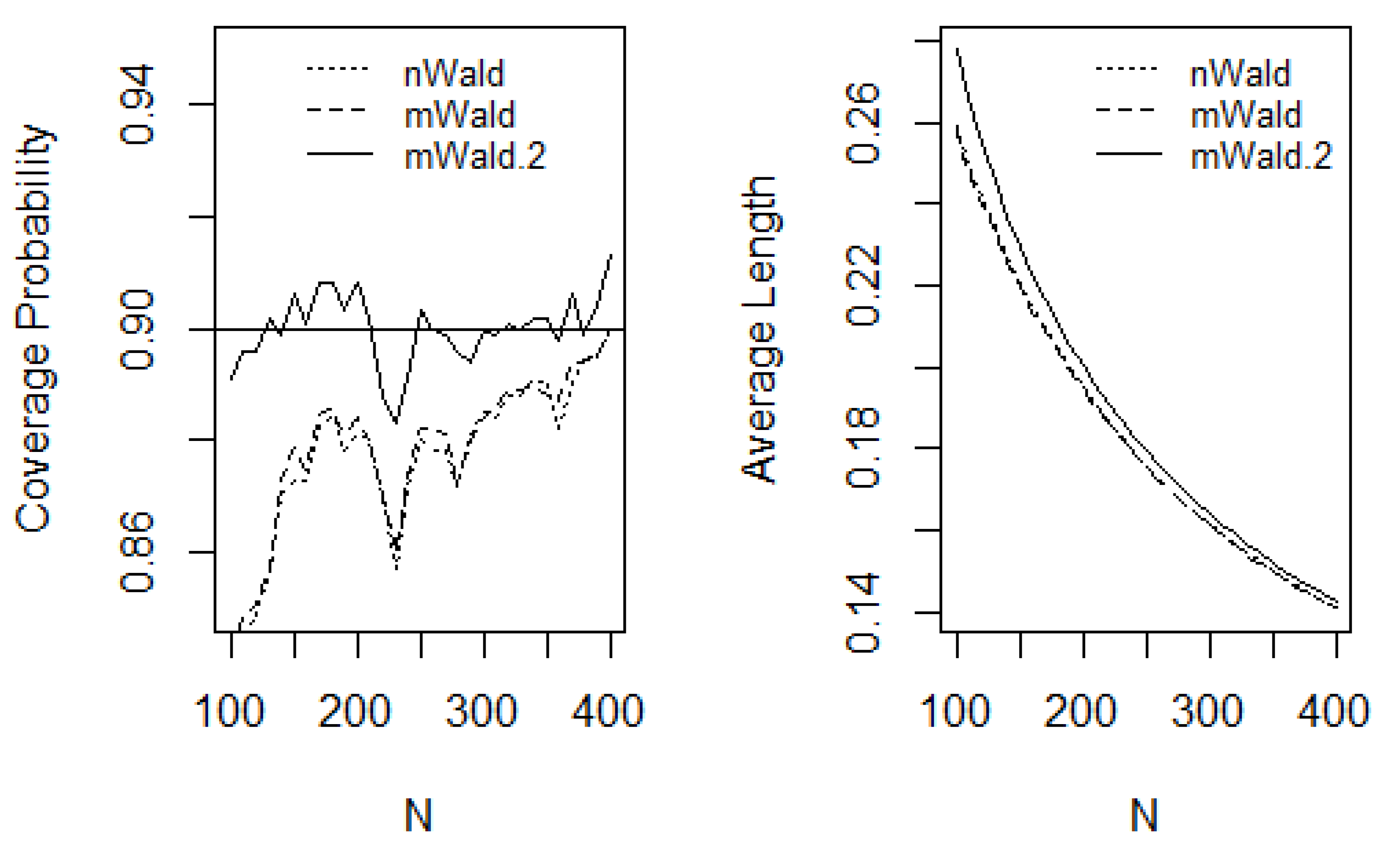
Figure 1 and Figure 2 display the plots of CPs and ALs for all CI methods as functions of N for the scenarios (p₁, p₂) = (0.4, 0.6) and (p₁, p₂) = (0.1, 0.2), respectively. When the true proportions are closer to 0.5—as in the case of (p₁, p₂) = (0.4, 0.6)—the underlying binomial distributions tend to be approximately symmetric around their means. This symmetry represents a “best-case” or “fair-coin” scenario in which the CI methods are generally expected to perform well. Persistently, across the entire range of sample sizes considered, Figure 1 shows that all three CI methods maintain CPs close to the nominal level, with the mWald.2 method performing particularly well. The nWald and mWald methods appear more conservative, as they converge more slowly to the nominal 90% CP—only reaching it at around N = 275. In terms of ALs, all three methods exhibit similar performance. In contrast, when the true proportion parameters are farther from the “fair-coin” case—as in (p₁, p₂) = (0.1, 0.2)—the binomial distributions become increasingly skewed, and their behavior becomes less favorable for inference. Under such conditions, particularly for small sample sizes, the CI methods are not expected to perform as reliably, and coverage may deviate from the nominal level.

The plots in Figure 2 illustrate that both the nWald and mWald CIs exhibit poor CPs when sample sizes are small. Their CPs approach the nominal level only as sample sizes become large. Remarkably, the mWald.2 method maintains consistently strong coverage across all sample sizes, with its CPs fluctuating closely around the nominal 90% level—even when N is as low as 100. For all three methods, the ALs are comparable throughout the sample size range.

The following provides guidance on the sample size ranges for which the three CI methods yield valid coverage. For the mWald.2 CI, when (p₁, p₂) = (0.4, 0.6), representing a “fair-coin” or best-case scenario, the CPs remain close to the nominal level, ranging approximately between 89% and 91%, even with total sample sizes as low as N > 100. Similarly, for the more challenging case of (p₁, p₂) = (0.1, 0.2), where the proportions are farther from 0.5, the mWald.2 method still maintains reasonable coverage (approximately 88% to 91%) for sample sizes N > 100.

For the other two CI methods, nWald and mWald, achieving coverage probabilities close to the nominal 90% level (approximately between 87% and 91%) requires larger sample sizes. When (p₁, p₂) = (0.4, 0.6), both methods require at least N > 250. In the more challenging case of (p₁, p₂) = (0.1, 0.2), acceptable coverage is attained only when N > 300.

Our simulations indicate that the mWald.2 CI method outperforms the other two methods, as it consistently maintains coverage probabilities close to the nominal level, even for relatively smaller sample sizes. Therefore, our findings align with the recommendations and conclusions of Agresti and Coull (1998) [14] and Lee and Byun (2008) [15].

6. Multiple Pairwise Comparisons (MPCs) in the Presence of Misclassified Binomial Data

When misclassified binomial data (including both false positives and false negatives) are present in pairwise comparisons involving more than two groups, as outlined in Section 2, Section 3, Section 4 and Section 5, a multiplicity issue arises. This issue, whether related to hypothesis testing or confidence intervals, stems from the repeated comparisons made between each pair of g groups. Therefore, it is essential to address this multiplicity problem. The typical objective is to control the family-wise error rate (FWER). This refers to the likelihood of committing at least one Type I error among the multiple pairwise comparisons. Consequently, it is essential to keep the FWER at a specified overall threshold, known as α. Numerous methods for MPC procedures, such as Bonferroni, Šidák, and Dunn, are available in the literature to achieve this control. These MPC adjustment techniques vary in how they modify the α value to account for the effects of multiple comparisons.

In this manuscript, we utilize three adjustment techniques—Bonferroni, Šidák, and Dunn—to account for differences in proportion parameters while considering both types of misclassifications (false positives and false negatives) in multiple-sample binomial data during the final calculation of CIs.

It is important to note that given there are g groups, the unique number of comparison pairs (combinations, not permutations) is as follows:

$$m=\left({\displaystyle \genfrac{}{}{0pt}{}{g}{2}}\right)=g(g-1)/2.$$

(6)

Additionally, it is essential to note that when we compare with a control group, the number of comparisons conducted is limited to the following:

$$m=\left(g-1\right).$$

(7)

As a result, when $m$ ≠ 1 for the pairs (and m is a positive integer), testing each pair at an overall significance level of α = 0.05 is no longer a fair or valid comparison (i.e., too lenient) because when we perform hypothesis testing multiple times (over and over again), it will be progressively easier for such multiple tests to be significant, and hence the overall α level should be penalized more stringently. Each pair must have its α significance level adjusted accordingly. The methods for the adjustment are outlined below.

6.1. Bonferroni Adjustment of CI for Misclassified Binomial Data

In the realm of machine learning, Salzberg (1997) [17] identifies the Bonferroni correction technique as a general approach to addressing the issue of multiple testing, with references to Hochberg (1988) [18], Holland (1991) [19], and Hommel (1988) [20], who also discuss this method. Salzberg points out that while the Bonferroni correction is the earliest and simplest method for understanding multiple testing, it tends to be overly conservative, making it slow to reject the null hypothesis of equality tests, and it may produce weak results due to its reliance on the assumption of independence among hypotheses. Nevertheless, we have opted to use the Bonferroni correction first when dealing with over-reported and/or under-reported binomial data. This correction operates as a single-step procedure, meaning that all CIs are compared against the same CI threshold across the m-adjusted intervals (Holland and Copenhaver, 1987 [21]; Hochberg and Tamhane, 1987 [22]).

To achieve an overall confidence level of (1 − α) × 100%, the Bonferroni adjustment procedure applied in a single step for each of the m individual CIs for δ is as follows:

$$\left(1-{\displaystyle \frac{\alpha }{m}}\right)\times 100\mathrm{\%},$$

(8)

where m is derived from Equation (6). If zero lies within the (adjusted) interval defined in Equation (8), we do not reject the equality of the pair’s proportions. Conversely, if zero is outside the (adjusted) interval (8), it indicates a significant difference between the pair’s proportions at each significance level of α/m (Bonferroni adjusted).

Using the Bonferroni adjustment outlined in Equation (8), with m specified in Equation (6), we analyze the North Carolina Traffic Data categorized into g = 4 groups (A = Male High Damage, B = Female High Damage, C = Male Low Damage, and D = Female Low Damage). This results in m = 6 (mWald.2) CIs, which are presented in

Table 5. mWald.2 method for overall 90% CIs (i.e., Bonferroni 98.33% CI or Sidak 98.26% CI for each group’s pair) for the traffic accident misclassified dataset.

Adjustment	Group’s Pair	CI	Zero in CI?	Significantly Different?
Bonferroni	AB	(−0.2448, −0.1044)	No	Yes
(98.33% CI)	AC	(0.169, 0.263)	No	Yes
	AD	(0.0850, 0.2062)	No	Yes
	BC	(0.323, 0.457)	No	Yes
	BD	(0.242, 0.397)	No	Yes
	CD	(−0.1270, −0.0137)	No	Yes
Sidak	AB	(−0.2443, −0.1049)	No	Yes
(98.26% CI)	AC	(0.170, 0.263)	No	Yes
	AD	(0.0854, 0.2058)	No	Yes
	BC	(0.324, 0.457)	No	Yes
	BD	(0.243, 0.396)	No	Yes
	CD	(−0.1266, −0.0141)	No	Yes

.

Table 5 illustrates that, when applying the Bonferroni adjustment method outlined in Equation (8), significant differences are identified in all pairs, as zero falls outside the Bonferroni-adjusted intervals for all these pairs. To attain an overall 90% CI with α = 0.1, the single-step Bonferroni adjustment method yields a Bonferroni CI of 98.33% for all of the m = 6 (mWald.2) CIs.

6.2. Šidák Adjustment of CI for Misclassified Binomial Data

Like the Bonferroni correction, the Šidák correction introduced in 1967 [23] is another widely used single-step method for adjusting multiple tests to control the FWER. However, this method is applicable only when the tests are independent or positively dependent. As with other single-step procedures, it involves comparing all CIs to the same CI threshold across each of the m-adjusted intervals for every zero tested.

To achieve an overall confidence level of (1 − α) × 100%, the single-step Šidák adjustment or correction technique for each m individual CI for δ is formulated as follows:

$$\left({\left(1-\alpha \right)}^{1/m}\right)\times 100\mathrm{\%},$$

(9)

where m is from Equation (6). If zero falls within the adjusted interval in Equation (9), we do not reject the equality of the pair’s proportions. Conversely, if zero is not included in the adjusted interval (9), it indicates a significant difference between the pair’s proportions at each significance level adjusted by Šidák, specifically at the $\left(1-{\left(1-\alpha \right)}^{1/m}\right)$ level.

By using the Šidák adjustment in Equation (9), along with m from Equation (6), for the North Carolina Traffic Data categorized into g = 4 groups (A = Male High Damage, B = Female High Damage, C = Male Low Damage, and D = Female Low Damage), we derive m = 6 (mWald.2) CIs, as presented in Table 5.

Table 5 illustrates that when applying the Šidák adjustment method as outlined in Equation (9), significant differences are found in all pairs. In this case involving traffic data, the results align with those obtained using the Bonferroni adjustment method detailed in Equation (8). To achieve an overall 90% CI (or α = 0.1), the single-step Šidák adjustment method yields a Šidák CI of 98.26% for each of the m = 6 (mWald.2) CIs.

6.3. Dunn Adjustment of CI for Misclassified Binomial Data

A widely used single-step adjustment method for corrections is the Dunn method (Dunn, 1961 [24]), which manages the family-wise error rate (FWER) by dividing α by m, the total number of comparisons conducted, where m is specified in Equation (7). This approach involves selecting one group as the control and comparing all other groups against it. The remainder of this procedure is straightforward to apply, as it follows the same protocol as the previously mentioned Bonferroni method outlined in Equation (8) of Section 6.1 but utilizes m from Equation (7) instead.

In this manuscript, we do not implement this adjustment or correction method to the traffic data because we do not designate any of the four groups (A, B, C, or D) as a control (placebo) group, akin to the typical approach taken in drug development (pharmaceutical studies).

7. Key Distinction of the Expanded Framework

In this section, we emphasize the key distinctions between the single-type misclassification framework proposed by Rahardja (2020) [10] and the broader expanded framework introduced in this paper, which simultaneously includes both types of misclassifications. The differences are outlined as follows:

• The former “NA” in the upper right 2 × 2 submatrix of Table 1 from Rahardja (2020) [10] has now been replaced with a subsample size of n_i10, leading to a change in the column total to n_i∙0.
• Similarly, the previous “NA” in the upper right 2 × 2 submatrix of the corresponding Table 2 from Rahardja (2020) [10] has been substituted with p_i θ_i.
• Previously, Equation (1) from Rahardja (2020) [10] depended solely on three parameters (p_i, q_i, ${\varphi }_i)$. It has now been expanded to include an additional parameter, ${\theta }_i,$ transforming it into a function of four parameters (p_i, q_i, ${\varphi }_i,$ ${\theta }_i$). Correspondingly, all subsequent equations derived are now functions of four parameters, along with the narratives that explain these newly derived equations in the manuscript.
• The former model described in Section 3 of Rahardja (2020) [10] utilized a trinomial distribution, whereas the enhanced model adopts a quadrinomial distribution. Consequently, the enhanced model includes two reparameterization formulas, as shown in Equation (4), compared to only one in the earlier model.
• The example in Section 4 of Rahardja (2020) [10] illustrated a single type of misclassification involving three parameters. In contrast, the example presented in this paper demonstrates both types of misclassifications involving four parameters.
• Additionally, the simulation in Section 5, which previously involved three parameters, now incorporates four parameters.
• Consequently, the previous adjustment level mentioned in Section 6, which solely addressed a single type of misclassification (one-sided level), has now accounted for both types of misclassifications (two-sided level) in multiple-sample binomial data.

8. Discussion and Conclusions

In this manuscript, we first develop three MLE methods (presented in the first stage, Section 2, Section 3 and Section 4) to estimate the proportion difference between two independent binomial samples in the presence of misclassifications. In Section 5, we conduct simulations to demonstrate the performance of these three MLE methods under binomial misclassifications. In the second stage (Section 6), we adjust the interval width to account for the multiplicity effect in MPCs. Subsequently, we highlight the key differences in Section 7 between the former framework of a single type of binary misclassification introduced in the previous literature [10] and the expanded framework developed in this paper, which includes both types of binomial misclassifications.

In the first stage (Section 2, Section 3 and Section 4), we employ a double sampling scheme to obtain additional information, ensure model identifiability, and reduce bias. During this process, we reparametrize the original full likelihood function, leading to a closed-form likelihood function that is computationally feasible. Without this reparameterization, such a closed-form expression would be computationally unattainable. As a result, the MLE and the corresponding three CI methods—nWald, mWald, and mWald.2—can be computed when evaluating the proportion difference.

In Section 5, during the simulations for the first stage, we apply the three CI methods to the large sample dataset from Hochberg (1977) [16] (shown in Table 4), focusing on Group A (Male, High Car Damage) and Group B (Female, High Car Damage). As expected, the three methods produce similar CIs due to the large sample sizes in the Hochberg dataset. It is worth noting that previous studies by Agresti and Coull (1998) [14] and Lee and Byun (2008) [15] have shown that adding one or two counts to the cell counts in small sample binomial data can help correct bias. This explains why, among the three likelihood-based methods, the mWald.2 method performs the best—its CPs consistently stay closest to the nominal values across all simulated scenarios, even with small sample sizes.

In the second stage (Section 6), to address the multiplicity effect in MPCs, we incorporate three adjustment methods—Bonferroni, Sidak, and Dunn—into the calculation of adjusted CIs for the differences in proportion parameters. These adjustments account for both types of misclassifications in multiple-sample binomial data.

As an illustration of the second stage, we apply the adjustment methods to the pairwise comparisons using MPCs on the large sample dataset from Hochberg (1977) [16], which includes four groups: Group A (Male and High Car Damage), Group B (Female and High Car Damage), Group C (Male and Low Car Damage), and Group D (Female and Low Car Damage). In this example, both the Bonferroni and Sidak adjustment methods reveal significant differences across all pairs.

As a recap, Section 7 pointed out the key distinctions between the single-type binomial misclassification framework introduced by Rahardja (2020) [10] and the broader framework discussed in this manuscript, which simultaneously accounts for both types of misclassifications.

In conclusion, we propose likelihood-based estimation methods to obtain confidence intervals (CIs) for comparing pairwise proportion differences under three multiplicity adjustment methods (Bonferroni, Sidak, and Dunn) in the context of misclassified multiple-sample binomial data using a double sampling scheme. These MPC methods will be valuable tools for practitioners and researchers working in the field of binomial misclassification.