Communication

Modeling Sea Level Rise Using Ensemble Techniques: Impacts on Coastal Adaptation, Freshwater Ecosystems, Agriculture and Infrastructure

by
Sambandh Bhusan Dhal
1,†,
Rishabh Singh
2,†,
Tushar Pandey
3,†,
Sheelabhadra Dey
4,†,
Stavros Kalafatis
1 and
Vivekvardhan Kesireddy
5,*
1
Department of Electrical and Computer Engineering, Texas A&M University, College Station, TX 77843, USA
2
Department of Biological and Agricultural Engineering, Texas A&M University, College Station, TX 77843, USA
3
Department of Mathematics, Texas A&M University, College Station, TX 77843, USA
4
Department of Computer Science and Engineering, Texas A&M University, College Station, TX 77843, USA
5
Department of Petroleum Engineering, Texas A&M University, College Station, TX 77843, USA
*
Author to whom correspondence should be addressed.
These authors contributed equally to this work.
Analytics 2024, 3(3), 276-296; https://doi.org/10.3390/analytics3030016
Submission received: 6 May 2024 / Revised: 9 June 2024 / Accepted: 26 June 2024 / Published: 5 July 2024

Abstract

:
Sea level rise (SLR) is a crucial indicator of climate change, primarily driven by greenhouse gas emissions and the subsequent increase in global temperatures. The impact of SLR, however, varies regionally due to factors such as ocean bathymetry, resulting in distinct shifts across different areas compared to the global average. Understanding the complex factors influencing SLR across diverse spatial scales, along with the associated uncertainties, is essential. This study focuses on the East Coast of the United States and Gulf of Mexico, utilizing historical SLR data from 1993 to 2023. To forecast SLR trends from 2024 to 2103, a weighted ensemble model comprising SARIMAX, LSTM, and exponential smoothing models was employed. Additionally, using historical greenhouse gas data, an ensemble of LSTM models was used to predict real-time SLR values, achieving a testing loss of 0.005. Furthermore, conductance and dissolved oxygen (DO) values were assessed for the entire forecasting period, leveraging forecasted SLR trends to evaluate the impacts on marine life, agriculture, and infrastructure.

1. Introduction

The steady rise in global sea levels (SLR) is a prominent consequence of climate change, closely linked to the increase in global temperatures [1]. This phenomenon primarily results from the expansion of ocean waters due to warming temperatures and the melting of glaciers and polar ice caps. However, the impact of SLR varies regionally due to complex interactions between oceanic features and various contributing factors. This variability introduces uncertainties, leading to divergent regional sea level patterns that deviate from the global average [2,3].
This paper aims to illuminate the multifaceted dynamics governing sea levels across various spatial scales, delving into the intricacies and the inherent uncertainties that define them. A comprehensive predictive model has been introduced, meticulously crafted to forecast SLR trajectories in response to greenhouse gas emissions [4]. This model not only predicts future trends but also vividly illustrates the potential consequences of SLR, with a particular focus on salinity and Biological Oxygen Demand—key indicators that shape oceanic habitats and, by extension, the ocean economy [5,6].
In the past, various modeling approaches have been employed to forecast SLR based on historical data and future scenarios. One commonly used technique involves the utilization of numerical models, which simulate the physical processes driving SLR. These models incorporate factors such as thermal expansion of seawater, melting of polar ice caps and glaciers, and changes in land ice dynamics [7,8,9]. By assimilating data from satellites, tide gauges, and oceanographic measurements, these models can accurately simulate past SLR trends and provide projections for future scenarios under different climate change scenarios [10,11].
Statistical models have played a significant role in predicting SLR. By analyzing historical data, these models identify trends and patterns in sea level variability, allowing researchers to establish statistical relationships between SLR and factors such as greenhouse gas emissions, global temperature, and oceanic conditions. Extrapolating these relationships into the future enables statistical models to forecast SLR trends and assess the likelihood of various scenarios [12,13,14,15].
In addition, machine learning (ML) techniques, including artificial neural networks (ANNs) and ensemble methods, have emerged as powerful tools for SLR prediction [16]. These models can capture complex non-linear relationships between diverse climate variables and SLR, resulting in more accurate and robust predictions. By training on large datasets of historical climate and sea level data, ML models can learn to forecast SLR patterns and identify the key drivers of future sea level projections.
Overall, predictive models have been instrumental in advancing our understanding of SLR dynamics and informing decision-making processes related to climate change adaptation and mitigation [17,18]. By integrating data-driven modeling approaches with physical principles and climate scenarios, researchers can develop more accurate and reliable predictions of future SLR trends, helping to guide policymakers, planners, and coastal communities in their efforts to prepare for and respond to the impacts of climate change.
Beyond the realm of physical science, this approach encompasses the socio-economic dimensions of SLR, incorporating factors such as population density and the resilience of infrastructural networks [19]. This integrative methodology provides a more nuanced projection, enabling stakeholders in coastal regions to engage in proactive management and adaptation strategies [20,21]. The cornerstone of this research is the rigorous analysis of historical data, which, combined with contemporary monitoring and data acquisition, refines the predictive models and enhances the understanding of sea level behavior [22].
The primary aim of this analysis is to examine the historical patterns of SLR and discern the human influence on climatic systems [23]. Through predictive modeling, the study aims to uncover patterns and trends, providing insights into the implications of SLR for both human settlements and ecological networks [24,25]. To achieve this, the research maps the communities at the forefront of these transformations.
Looking beyond the immediate horizon, the research aims to harness data-driven methodologies to enhance predictive capabilities and develop robust strategies to mitigate the impacts of climate change on humanity and the natural world.

2. Materials and Methods

2.1. Construction of the Dataset
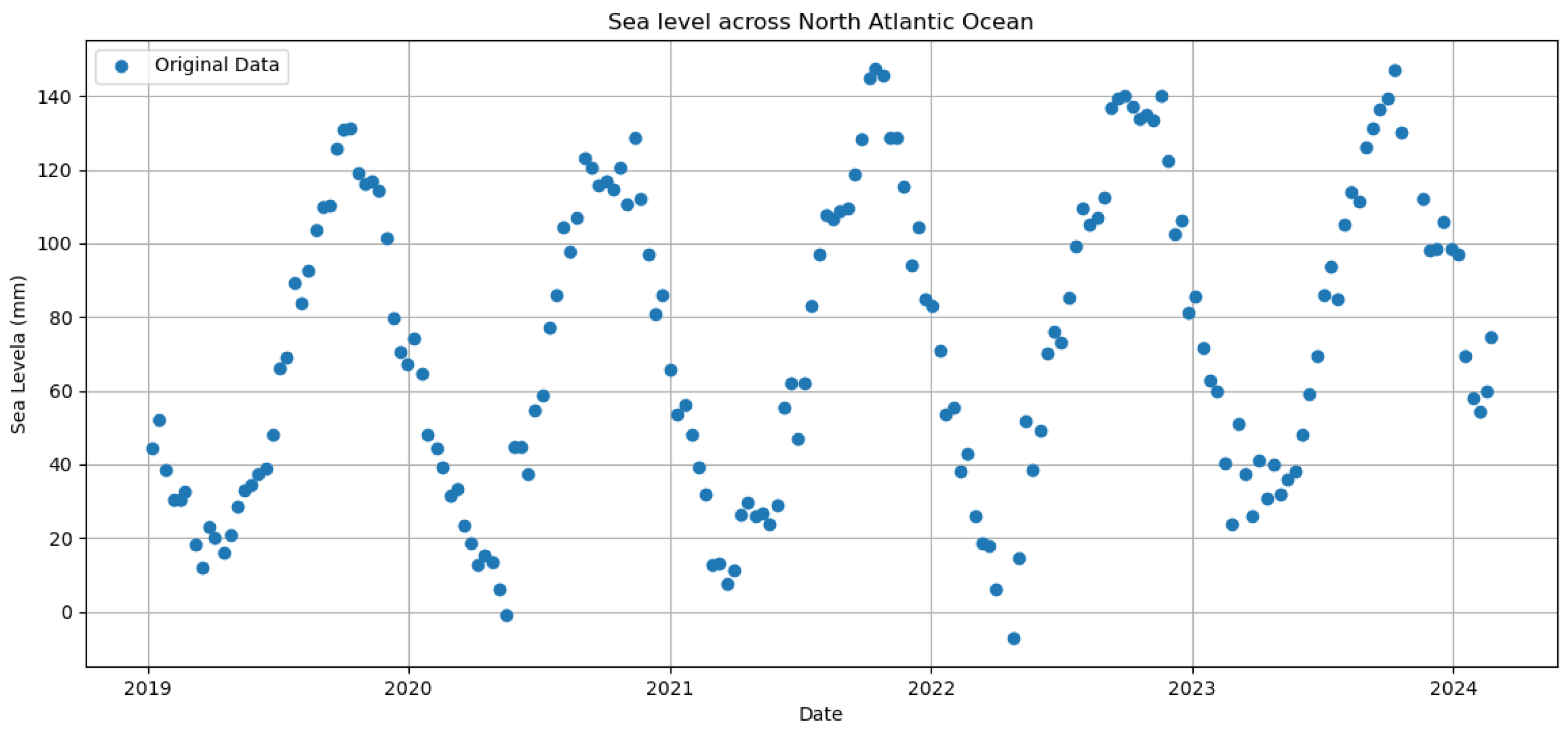
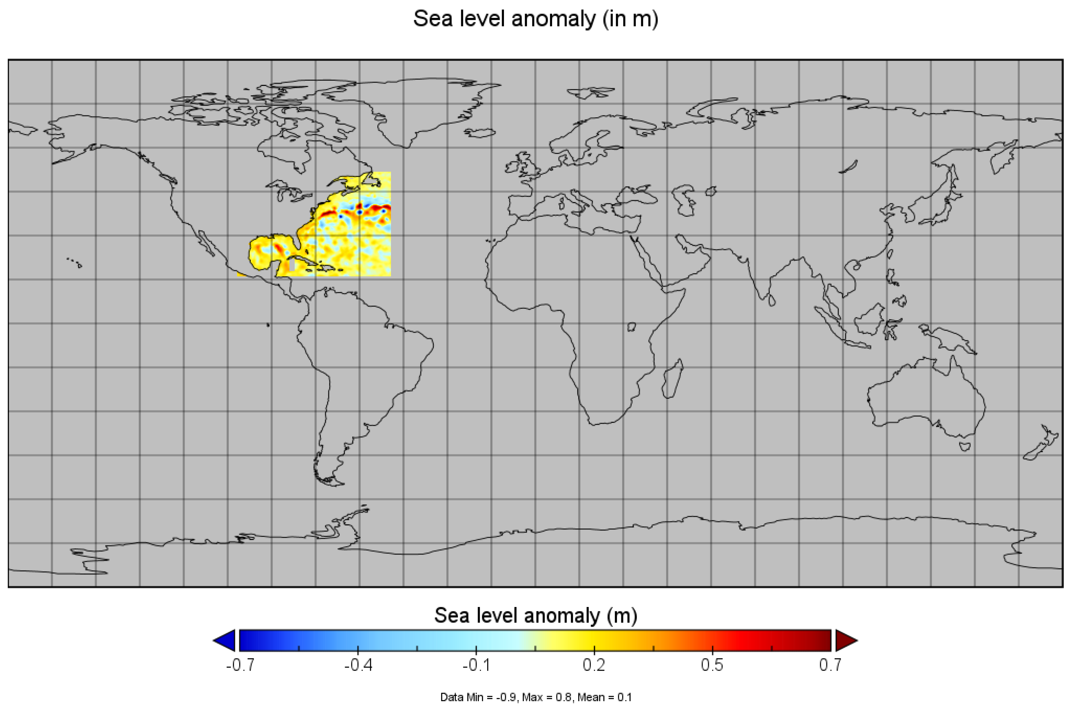
2.1.1. Study Area

The study area comprises the states of Texas, Louisiana, Mississippi, Alabama, Florida, Georgia, North Carolina, South Carolina, Virginia, Delaware, New Jersey, New York, Connecticut, Rhode Island, Massachusetts, Maine, and Pennsylvania. The states encompass the Gulf of Mexico and the Eastern Coast of the Contiguous United States (CONUS) adjacent to the North Atlantic Ocean. Low-lying coastal areas are among the most vulnerable to the effects of sea level rise, with a total population of almost 300 million living along the coasts of the globe, including 20 of the 33 megacities [26]. With dense population and development along the coastline, these states, at present, are highly vulnerable to coastal flooding [27]. SLR is predominantly driven by the thermal expansion of seawater due to global warming and the melting of ice caps and glacier sheets, leading to increased sea levels. While several short-term responses and adaptation options exist, it was imperative to consider long-term strategies for both public infrastructure and private development. The coastline used in this study has been depicted in Figure 1.
Prior to delving into the detailed analysis of SLR, it was essential to examine the seasonal trends in sea levels. To achieve this, a five-year period (2019–2024) was selected, and seasonal variations along the North Atlantic Ocean region have been observed, as depicted in Figure 2.
From Figure 2, it was observed that the seasonal fluctuations in sea levels are markedly pronounced, with winter months exhibiting notably lower sea levels, while summer months consistently present elevated levels. The annual cycle reached its lowest sea levels in March, characterizing the seasonal minima, and ascended to its peak during August and September, marking the seasonal maxima. This cyclical pattern underscored the significant impact of seasonal changes on marine water levels and is expected to be this way for a few more decades.

2.1.2. Sea Level Rise

SLR data were sourced from the National Oceanic and Atmospheric Administration’s (NOAA)/NESDIS/STAR Laboratory for Satellite Altimetry website, encompassing data from all altimeter missions including Copernicus (Sentinel-6A, Sentinel-3A), Jason-3, and Topex/Poseidon. The dataset covered the period from 1993 to 2023 and was obtained in netCDF format for analysis in ArcGIS Pro. Additional visualization data were acquired from Copernicus Climate Change (C3) Services. The variables “Absolute Dynamic Topography (ADT)” and “Sea Level Anomaly (SLA)” for the same period were utilized to examine SLR trends in the Gulf of Mexico and North Atlantic Ocean along the Southeastern and Eastern US Coast.
SLR represented by ADT denotes the gradual, long-term elevation in the average level of the ocean’s surface, primarily driven by climate-change-induced phenomena such as thermal expansion and melting ice caps. It is a global phenomenon with significant implications for coastal regions worldwide. Conversely, SLA refers to short-term fluctuations in sea level, deviating from the average at specific locations and times due to various factors like ocean currents, atmospheric pressure, and gravitational effects. While SLR poses a persistent threat to coastal communities and ecosystems, SLAs can cause temporary fluctuations that may impact coastal infrastructure and maritime activities.
The plots for ADT and SLA are shown in Figure 3 and Figure 4, respectively.

2.1.3. Greenhouse Gases Contributing to SLR

Before analyzing the impact of SLR, it was important to gauge the different factors contributing to the rise in sea level. For this, the different pollutants emitted from industrial processes, power plants, vehicle exhausts, and biomass burning were visualized. The initial dataset which was used contained greenhouse gas data like Sulfur Dioxide (SO2), Carbon Monoxide (CO), Carbon Dioxide (CO2), particulate matter 10 (PM10), and particulate matter (PM2.5), and their cumulative concentrations over the years; which are as shown in Figure 5. As these pollutants contribute to increasing global warming and SLR, the reasons for selecting these pollutants have been shown in Table 1.

2.1.4. Specific Conductance

The Coastal Data and Analysis Tool for Water Resources Management (CDAT-WRM) provided specific conductance data for visualizations related to coastal water management. This tool integrates features from two U.S. Geological Survey websites: the Water Level and Salinity Analysis Mapper and the Coastal Salinity Index [28]. The specific conductance values were aggregated from daily readings and represent the mean value.

2.1.5. Dissolved Oxygen (DO)

From the globally gridded dataset of DO in surface water for the period 1993–2010, monthly observations were downloaded from The World Bank Data Catalog [29] for Chesapeake Bay, which is the largest estuary in the United States.

2.2. Preprocessing of Dataset

Various interpolation techniques were employed on the SLR datasets to construct a chronological series, facilitating the development of a predictive model. For this analysis, the counties with populations exceeding 100,000 were prioritized along the coastline. Missing values were imputed using the arithmetic mean method, applying percentages rather than aggregate figures [30]. The temporal scope of the greenhouse gas datasets was standardized to align with the SLR data. Subsequently, multiple datasets were amalgamated, focusing on features and effects correlated with SLR to support future visualization efforts.

2.3. Analysis of the Dataset

Initially, the influence of greenhouse gases on SLR was investigated. For this, an ensemble of 5 LSTM models was used to find the most optimal model in predicting SLR (along the East Coast and Gulf of Mexico) based on their testing accuracy [31]. This model was instrumental in determining the predictive weights for future SLR projections, contingent upon variable greenhouse gas levels influenced by governmental policies and strategies. A weighted hybrid model combining Long Short-Term Memory (LSTM) and Seasonal Autoregressive Integrated Moving Average with Exogenous Regressors (SARIMAX) methodologies [32] was used exclusively for SLR projections to anticipate the future impact on land and water resources in coastal counties. Extensive visualizations were generated, including representations of GDP percentage shifts within specific economic sectors across multiple eastern coastal counties. Network analysis was conducted, culminating in the creation of a dynamic 3D graph [33] featuring searchable nodes and highlighting capabilities. This analysis aimed to elucidate the correlation between SLR trends and regional pollutants over time. Ultimately, leveraging this model, an interactive tool was designed capable of predicting SLR outcomes based on user-inputted pollutant levels, projecting up to the year 2103. This comprehensive project offered insights into the potential ramifications of climate policy on global warming, with a particular focus on SLR, thereby enabling predictions regarding its subsequent effects on biodiversity, water salinity, and agricultural conditions [34].

3. Results

Before conducting a detailed analysis, Figure 6 presents a schematic that explains the various predictive models used for real-time prediction of SLR as well as for forecasting SLR trends from 2024 to 2103. Details about each of the predictive models used are explained in detail in the sub-sections below.

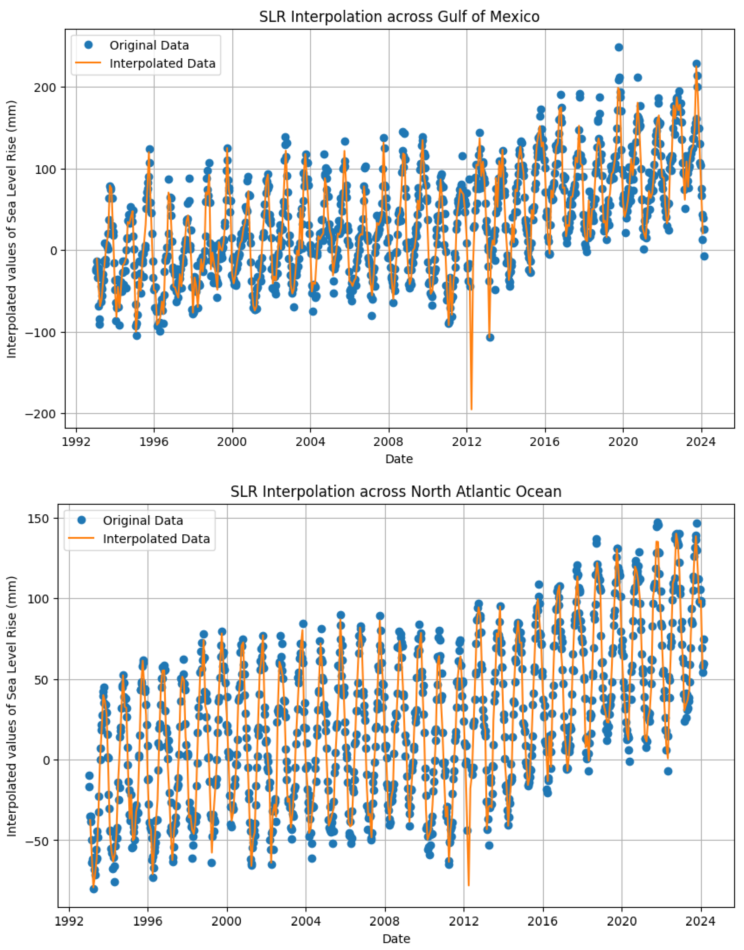
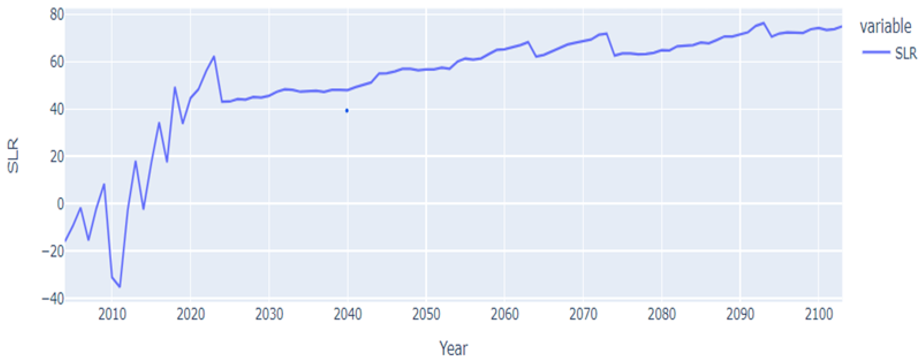
3.1. Sea Level Rise Modeling

One of the important parameters while trying to gauge the effects of SLR was to estimate it itself for the course of the next century. For that, the data that was used were available for the period from 1993 to 2023. As the data were recorded for roughly 45 days at irregular intervals for each year, it was imperative to interpolate the data points before carrying out the prediction analysis. To interpolate the data, it was decided to use a cubic-spline-based interpolation technique, as the dataset used was non-linear and exhibited seasonality. To have a better estimate of the interpolation, the dataset was divided into regions surrounding the Gulf of Mexico and the East Coast (i.e., the North Atlantic Ocean). The interpolated SLR data along the Gulf of Mexico and the East Coast have been depicted in Figure 7.
However, to predict the trend of the SLR over the course of the century, the average interpolated data over the Gulf of Mexico and the North Atlantic Ocean was used to design the approach. In this case, a combined forecast was generated by using an ensemble of a two-layered LSTM model, a SARIMA model, and an exponential smoothing model by assigning weights to each of their forecasts. The details of the weighted model used for forecasting the values have been depicted in Table 2.
The prediction analysis was performed as follows: The data from 1993 to 2023 were used to predict the SLR data from 2023 to 2043. After this, the predicted data until 2033 were appended to the original dataset, and the predictions were made from 2033 to 2053. This process was repeated until the SLR data were predicted until 2103. In this process, the data were averaged twice over every prediction period to obtain an estimate of the SLR trend over the next century. The major advantage of this technique was that as the data were predicted twice over every time period, the average of the data to obtain the forecasting trend gave a more accurate estimate. The predicted values of SLR from 2023 to 2103 have been shown in Figure 8.

3.2. Root Cause SLR Predictions

Before analyzing the impact of SLR, it was important to gauge the different factors contributing to the rise in sea level. For this, the different pollutants emitted from industrial processes, power plants, vehicle exhausts, and biomass burning were modelled. The initial dataset which was used contained greenhouse gas data like Sulfur Dioxide (SO2), Carbon Monoxide (CO), Carbon Dioxide (CO2), particulate matter 10 (PM10), and particulate matter (PM2.5). The pairwise correlation between these pollutants have been shown in Figure 9.
As the pairwise correlation between CO-CO2 and PM10-PM2.5 was very high (more than 80%), it was decided that PM2.5 and CO2 should be dropped before proceeding further with the regression analysis.
In this study, regression analysis was conducted using two distinct models. To predict SLR along the Gulf of Mexico, monthly predictor data spanning counties surrounding the Gulf from 1993 to 2023 were analyzed. Similarly, data from surrounding counties were utilized to predict SLR along the East Coast.
As the dataset at hand had monthly time-series data for all of the counties, it was decided to use an LSTM framework for prediction. However, due to the non-linear nature of the dataset, it was decided to use an ensemble approach comprising five LSTM models, and the best LSTM model was determined based on the model that had the lowest testing loss. In this case, the dataset was divided into training, validation, and testing at a ratio of 60:20:20.
The details of the LSTM model used are as follows:
  • Input layer (64 input neurons);
  • Three intermediate layers (64, 64, and 32 neurons, respectively);
  • One dense unit at the output;
  • Dropout of 0.2 after each layer followed by batch normalization;
  • Optimizer = ‘adam’, Loss = ‘mean squared error’.
The training, testing, and validation loss details of the LSTM model have been shown in Figure 10.
As observed from Figure 10, in order to predict the values of SLR along the Gulf of Mexico, model 2 was considered as it had the lowest test loss (0.0073). Similarly, to predict the values of SLR along the East Coast, an ensemble of the LSTM models was considered as the average testing loss was comparable at 0.005.

3.3. Analyzing the Effects of Sea Level Rise

3.3.1. Projected Conductivity

Based on the projected SLR trend (Figure 8), the trend of specific conductance was forecasted at three representative locations: (1) Collier County, Florida; (2) Cameron Parish County, Louisiana; and (3) Chester County, Pennsylvania, as illustrated in Figure 11. In these areas, freshwater conductivity, indicated by specific conductance, has shown an upward trend in recent years (solid blue lines). Assuming a proportional increase in freshwater conductivity with rising sea levels, the trends suggest that conductivity—and thus salinity—will likely rise in the coming decades (dotted orange line). This projected increase poses a significant challenge necessitating comprehensive management strategies. Addressing this issue proactively through monitoring, regulation, and investment in treatment technologies, alongside public education, will be crucial to mitigate the multifaceted impacts on the state’s environment, public health, agriculture, infrastructure, and economy.

3.3.2. Projected Dissolved Oxygen

SLR indirectly impacts biological oxygen demand (BOD) and dissolved oxygen (DO) through various factors such as increased organic matter input from erosion, altered hydrology affecting nutrient dynamics, habitat loss or shifts, changes in salinity, nutrient loading, and the promotion of hypoxic/anoxic conditions. These effects can lead to lower DO levels, harming aquatic life and ecosystem health in coastal areas. Understanding these interactions is crucial for managing the consequences of SLR on water quality and coastal environments.
The analysis presented in Figure 12 includes dissolved oxygen (DO) predictions influenced by the SLR trends in Chesapeake Bay, the largest estuary in the USA, and the Gulf of Mexico. Based on earlier SLR predictions, a notable decrease in DO is projected, reaching 1.4 mg/L in the Gulf of Mexico and 1.09 mg/L in Chesapeake Bay (East Coast) over 100 years. Chesapeake Bay stands out as one of the most vulnerable regions in the nation to the impacts of rising sea levels.
These are the reference levels for dissolved oxygen (DO).
  • Good Water Quality: DO levels above 8 mg/L are considered indicative of good water quality.
  • Moderate Water Quality: DO levels between 3 mg/L and 8 mg/L may indicate moderate pollution.
  • Poor Water Quality: DO levels below 3 mg/L suggest poor water quality and significant pollution.

4. Discussion

The electrical conductivity of water is a crucial measure of its ability to conduct electricity, which is directly influenced by the presence of dissolved salts and inorganic materials such as chlorides, sulfates, and bicarbonate ions [35]. High conductivity in water often indicates a high level of dissolved salts, which can have significant implications for water quality. For instance, the United States Geological Survey (USGS) highlights the importance of monitoring conductivity as an indicator of water quality, noting its impact on ecosystem health and water usability (USGS, Water Quality Information by Topic, 2023) [36]. Similarly, the Environmental Protection Agency (EPA) underscores conductivity as a key water quality parameter, particularly in the context of assessing the impact of pollution and urban runoff on aquatic environments (EPA, Conductivity: Electrical Conductivity in Water, 2023) [37].

4.1. Impact on Freshwater Aquatic Ecosystems

Most aquatic organisms can tolerate a specific range of salinity. The salinity of their surroundings shapes their physiological adaptation. Certain species, such as sea stars and sea cucumbers, are intolerant of low salinity levels and are typically absent from many estuaries. Additionally, some aquatic organisms are sensitive to the specific ionic composition of water. Even if salinity levels remain within an acceptable range, an influx of particular salts can adversely affect these species.
The tolerance of organisms to salinity depends on their osmotic processes. Freshwater organisms, characterized by low conductivity, are hyperosmotic, meaning they can expel water and retain ions, maintaining higher internal ionic concentrations than the surrounding water. Any alteration in the conductivity of the environment, such as changes in salt levels or types of ions, can negatively impact the metabolic functions of these organisms [38,39].

4.2. Impact on Agriculture

SLR contributes to increased soil electrical conductivity (EC) due to seawater intrusion into coastal soils, leading to higher salinity levels. This elevated soil salinity adversely affects agricultural productivity by impairing plant water uptake, resulting in reduced crop yields and compromised food security. Addressing this challenge requires innovative agricultural techniques and food processing methods to ensure food safety and quality.
To address increased soil salinity, precision agriculture can play a crucial role in managing soil health [40,41,42]. Techniques such as hydroponics and aquaponics, which control salinity and nutrient levels without relying on soil, offer viable alternatives for crop production under high-salinity conditions. These methods can mitigate the negative impacts of soil salinity on crop yields and contribute to sustainable food production [43,44,45,46,47,48,49,50].
Investigating solutions for food safety, non-thermal processing techniques, such as ozone treatment [51], present promising methods for ensuring the safety and quality of food products affected by high salinity levels. Ozone has demonstrated effective pathogen inactivation and reduction of contaminants such as biofilms, antibiotics, and aflatoxins in food products, while preserving their quality parameters. This positions ozone as a valuable tool for maintaining food safety amidst environmental changes induced by SLR. Additionally, advanced treatment technologies like atmospheric pressure cold plasma [52] and pulsed electric field techniques [53] can efficiently eliminate heavy metals from food products. These methods safeguard food safety and quality, addressing environmental contamination and disruptions affecting food production due to rising sea levels.
The valorization of agricultural and food waste presents another avenue for enhancing food security and sustainability. By extracting valuable bioactive compounds from agri-food waste, industries can create cost-effective, sustainable products that improve food quality and safety. Techniques such as ultrasound-assisted extraction and supercritical fluid extraction are particularly effective in isolating these compounds, aligning with the principles of a circular economy [54,55].
In summary, the increase in SLR and subsequent rise in soil conductivity and salinity pose significant challenges to food security. However, innovative agricultural practices, non-thermal food processing techniques, and the valorization of agri-food waste offer viable solutions to mitigate these impacts and ensure the continued safety and quality of food products.

4.3. Impact on Drinking Water

Conductivity in drinking water, indicative of its salinity level, has direct implications for human health and the palatability of water. High conductivity levels, resulting from elevated concentrations of dissolved salts and minerals, can lead to water tasting salty, which may discourage consumption and lead to dehydration or the consumption of less healthy alternatives [56,57,58]. More critically, certain dissolved ions, such as sodium and chloride, at high concentrations can pose health risks, particularly for individuals with hypertension or heart disease, as they can exacerbate these conditions. The World Health Organization (WHO) has established guidelines for the maximum concentrations of various dissolved ions in drinking water to safeguard public health. Ensuring that drinking water meets these guidelines requires monitoring and potentially treating water to remove excess salts, which can be costly but is essential for maintaining the health and well-being of communities.

4.4. Impact on Infrastructure

The impact of conductivity/salinity in water on infrastructure is significant and multifaceted. High levels of salinity in water can lead to corrosion and deterioration of infrastructure materials, including metals and concrete. This corrosion can compromise the structural integrity of buildings, bridges, and pipelines, leading to costly repairs and replacements. For instance, salt accelerates steel reinforcement corrosion in concrete, a process known as chloride-induced corrosion, which is a major concern for coastal and marine structures [59,60]. Additionally, salinity can affect the efficiency of water treatment plants by increasing the cost and complexity of water purification processes. These impacts underscore the importance of monitoring and managing salinity levels in water to protect and extend the lifespan of infrastructure.

5. Conclusions

In this study, an analysis of sea level rise (SLR) data was conducted along the East Coast and the Gulf of Mexico spanning from 1993 to 2023. Our primary objective was to develop accurate predictive models for real-time SLR values, considering greenhouse gas emissions as the primary drivers of global warming. To achieve this, an ensemble of Long Short-Term Memory (LSTM) models was employed, known for their ability to capture temporal dependencies in sequential data.
Subsequently, a weighted forecasting model comprising SARIMAX, LSTM, and exponential smoothing techniques was constructed to project SLR trends from 2024 to 2103. Additionally, this analysis extended to forecasting trends in conductance and dissolved oxygen (DO) values, which are critical factors influenced by SLR that significantly impact marine life. Beyond these environmental factors, the potential impacts of SLR on freshwater aquatic ecosystems, agriculture, drinking water, and infrastructure were also accessed.
Expanding on this analysis of SLR along the East Coast and the Gulf of Mexico, it is evident that greenhouse gas emissions are the primary drivers of global warming, consequently influencing SLR trends. To effectively mitigate SLR, it is imperative to implement targeted measures to reduce greenhouse gas emissions. One recommendation is to transition to renewable energy sources such as solar and wind power; meanwhile, enhancing energy efficiency in industries, transportation, and residential sectors can significantly curb emissions.
Moreover, coastal protection and adaptation strategies, such as mangrove restoration and robust coastal infrastructure, are crucial for mitigating the impacts of SLR. SLR increases soil salinity, which negatively affects agricultural productivity and food security. Innovative agricultural techniques, such as hydroponics and aquaponics, can help manage soil salinity. Additionally, non-thermal food processing methods, such as ozone treatment, ensure food safety. Advanced technologies like atmospheric pressure cold plasma and pulsed electric fields further enhance food safety by eliminating contaminants. To promote sustainability, agricultural waste can be valorized using techniques such as ultrasound-assisted and supercritical fluid extraction.
However, constructing accurate forecasting models with limited data poses several challenges. Insufficient data points hinder accurate pattern recognition, while limited data variability affects the generalization ability of the models. Moreover, the risk of overfitting increases with smaller sample sizes, and complex models built on limited data can become unstable, making feature selection challenging and hindering model validation and testing.
To address these challenges, future work could explore various strategies such as simplification, regularization, and careful feature engineering techniques. Different ensemble methods, data augmentation, and Bayesian approaches could also be utilized to improve model robustness and quantify uncertainty. Nonetheless, it is essential to acknowledge the inherent limitations of working with limited data and interpret the forecasts cautiously, considering potential inaccuracies and uncertainties in the predictions, and their subsequent impacts.

Author Contributions

Conceptualization, S.B.D., R.S., T.P., S.D., S.K., and V.K.; methodology, S.B.D., R.S., T.P., S.D., and V.K.; software, S.B.D., R.S., T.P., S.D., and V.K.; validation, S.B.D., R.S., T.P., S.D., and V.K.; formal analysis, S.B.D., R.S., T.P., S.D., S.K., and V.K.; investigation, S.B.D., R.S., T.P., S.D., S.K., and V.K.; resources, S.B.D., R.S., T.P., S.D., and V.K.; data curation, S.B.D., R.S., T.P., S.D., and V.K.; writing—original draft preparation, S.B.D., R.S., T.P., S.D., and V.K.; writing—review and editing, S.B.D., R.S., T.P., S.D., and V.K.; visualization, S.B.D., R.S., T.P., S.D., and V.K.; supervision, S.B.D., R.S., T.P., S.D., S.K., and V.K.; project administration, S.B.D., R.S., T.P., S.D., S.K., and V.K.; funding acquisition, S.B.D., R.S., T.P., S.D., and V.K. All authors have read and agreed to the published version of the manuscript.

Funding

This research received no external funding.

Institutional Review Board Statement

Not Applicable.

Informed Consent Statement

Not Applicable.

Data Availability Statement

All relevant data and code files have been made available at https://github.com/Sambandh/TAMIDS2024/tree/master (accessed on 5 May 2024).

Acknowledgments

The work was carried out as a part of the 2024 annual Data Science Competition organized by the Institute of Data Science, Texas A&M University.

Conflicts of Interest

The authors declare no conflicts of interest.

References

  1. Lumpkin, R.L. Climate Change: Global Sea Level. Reviewed By Rick. Available online: https://www.climate.gov/news-features/understanding-climate/climate-change-global-sea-level?utm_source=twitter.com&utm_medium=social&utm_campaign=sealevelrise%2Bwebsite (accessed on 5 May 2024).
  2. Wachler, B.; Seiffert, R.; Rasquin, C.; Kösters, F. Tidal response to sea level rise and bathymetric changes in the German Wadden Sea. Ocean. Dyn. 2020, 70, 1033–1052. [Google Scholar] [CrossRef]
  3. Jakobsson, M.; Mayer, L.A. Polar region bathymetry: Critical knowledge for the prediction of global sea level rise. Front. Mar. Sci. 2022, 8, 788724. [Google Scholar] [CrossRef]
  4. Garner, G.; Hermans, T.H.J.; Kopp, R.; Slangen, A.; Edwards, T.; Levermann, A.; Nowicki, S.; Palmer, M.D.; Smith, C.; Fox-Kemper, B.; et al. IPCC AR6 WGI Sea Level Projections; World Data Center for Climate (WDCC): Hamburg, Germany, 2022. [Google Scholar]
  5. Stramma, L.; Schmidtko, S. Tropical deoxygenation sites revisited to investigate oxygen and nutrient trends. Ocean. Sci. 2021, 17, 833–847. [Google Scholar] [CrossRef]
  6. Ashrafuzzaman, M.; Gomes, C.; Guerra, J. Climate justice for the southwestern coastal region of Bangladesh. Front. Clim. 2022, 4, 881709. [Google Scholar] [CrossRef]
  7. Notz, D. Challenges in simulating sea ice in Earth System Models. Wiley Interdiscip. Rev. Clim. Chang. 2012, 3, 509–526. [Google Scholar] [CrossRef]
  8. Allison, I.; Paul, F.; Colgan, W.; King, M. Ice sheets, glaciers, and sea level. In Snow and Ice-Related Hazards, Risks, and Disasters; Elsevier: Amsterdam, The Netherlands, 2021; pp. 707–740. [Google Scholar]
  9. Van Der Veen, C.J.; Payne, A.J. Modelling land-ice dynamics. In Mass Balance of the Cryosphere Observations and Modelling of Contemporary and Future Changes; Cambridge University Press: Cambridge, UK, 2004; pp. 169–219. [Google Scholar]
  10. Pickering, M.D.; Horsburgh, K.J.; Blundell, J.R.; Hirschi, J.M.; Nicholls, R.J.; Verlaan, M.; Wells, N.C. The impact of future sea-level rise on the global tides. Cont. Shelf Res. 2017, 142, 50–68. [Google Scholar] [CrossRef]
  11. Ponte, R.M.; Carson, M.; Cirano, M.; Domingues, C.M.; Jevrejeva, S.; Marcos, M.; Mitchum, G.; Van De Wal, R.S.W.; Woodworth, P.L.; Ablain, M.; et al. Towards comprehensive observing and modeling systems for monitoring and predicting regional to coastal sea level. Front. Mar. Sci. 2019, 6, 437. [Google Scholar] [CrossRef]
  12. Tebaldi, C.; Strauss, B.H.; Zervas, C.E. Modelling sea level rise impacts on storm surges along US coasts. Environ. Res. Lett. 2012, 7, 014032. [Google Scholar] [CrossRef]
  13. Lentz, E.E.; Thieler, E.R.; Plant, N.G.; Stippa, S.R.; Horton, R.M.; Gesch, D.B. Evaluation of dynamic coastal response to sea-level rise modifies inundation likelihood. Nat. Clim. Chang. 2016, 6, 696–700. [Google Scholar] [CrossRef]
  14. Plant, N.G.; Thieler, E.R.; Passeri, D.L. Coupling centennial-scale shoreline change to sea-level rise and coastal morphology in the Gulf of Mexico using a Bayesian network. Earth’s Future 2016, 4, 143–158. [Google Scholar] [CrossRef]
  15. Hauer, M.E.; Evans, J.M.; Mishra, D.R. Millions projected to be at risk from sea-level rise in the continental United States. Nat. Clim. Chang. 2016, 6, 691–695. [Google Scholar] [CrossRef]
  16. Bahari, N.A.A.B.S.; Ahmed, A.N.; Chong, K.L.; Lai, V.; Huang, Y.F.; Koo, C.H.; Ng, J.L.; El-Shafie, A. Predicting sea level rise using artificial intelligence: A review. Arch. Comput. Methods Eng. 2023, 30, 4045–4062. [Google Scholar] [CrossRef]
  17. Hall, J.A.; Weaver, C.P.; Obeysekera, J.; Crowell, M.; Horton, R.M.; Kopp, R.E.; Marburger, J.; Marcy, D.C.; Parris, A.; Sweet, W.V.; et al. Rising sea levels: Helping decision-makers confront the inevitable. Coast. Manag. 2019, 47, 127–150. [Google Scholar] [CrossRef] [PubMed]
  18. Nicholls, R.J.; Hanson, S.E.; Lowe, J.A.; Slangen, A.B.A.; Wahl, T.; Hinkel, J.; Long, A.J. Integrating new sea-level scenarios into coastal risk and adaptation assessments: An ongoing process. Wiley Interdiscip. Rev. Clim. Chang. 2021, 12, e706. [Google Scholar] [CrossRef]
  19. Khojasteh, D.; Haghani, M.; Nicholls, R.J.; Moftakhari, H.; Sadat-Noori, M.; Mach, K.J.; Fagherazzi, S.; Vafeidis, A.T.; Barbier, E.; Shamsipour, A.; et al. The evolving landscape of sea-level rise science from 1990 to 2021. Commun. Earth Environ. 2023, 4, 257. [Google Scholar] [CrossRef]
  20. Titheridge, H.; Parikh, P. Selected Conference Proceedings: 3rd International Conference on Urban Sustainability and Resilience; UCL: London, UK, 2017. [Google Scholar]
  21. Avron, L.A. Knowing and Responding: Localizing Climate Predictions in Florida; Cornell University: Ithaca, NY, USA, 2021. [Google Scholar]
  22. Tur, R.; Tas, E.; Haghighi, A.T.; Mehr, A.D. Sea level prediction using machine learning. Water 2021, 13, 3566. [Google Scholar] [CrossRef]
  23. Ranasinghe, R. Climate Change 2021: Summary for All. 2022. Available online: https://ris.utwente.nl/ws/portalfiles/portal/294260489/IPCC_AR6_WGI_SummaryForAll.pdf (accessed on 5 May 2024).
  24. Adshead, D.; Akay, H.; Duwig, C.; Eriksson, E.; Höjer, M.; Larsdotter, K.; Svenfelt, Å.; Vinuesa, R.; Nerini, F.F. A mission-driven approach for converting research into climate action. npj Clim. Action 2023, 2, 13. [Google Scholar] [CrossRef]
  25. Sebestyén, V.; Czvetkó, T.; Abonyi, J. The applicability of big data in climate change research: The importance of system of systems thinking. Front. Environ. Sci. 2021, 9, 619092. [Google Scholar] [CrossRef]
  26. Griggs, G.; Reguero, B.G. Coastal adaptation to climate change and sea-level rise. Water 2021, 13, 2151. [Google Scholar] [CrossRef]
  27. Crossett, K.M. Population Trends along the Coastal United States: 1980–2008; US Department of Commerce, National Oceanic and Atmospheric Administration, National Ocean Service, Management and Budget Office, Special Projects: Washington, DC, USA, 2004; Volume 55. [Google Scholar]
  28. Inventory and Appraisal of Glaciers in the St. Elias Mountains, Alaska and Yukon Territory, Canada, and Selected other Glaciers in Alaska: Description of Digital Geospatial Database. U.S. Geological Survey. Available online: https://pubs.usgs.gov/publication/70221055 (accessed on 5 May 2024).
  29. World Bank. Data Catalog. World Bank. Available online: https://datacatalog.worldbank.org/ (accessed on 5 May 2024).
  30. Sangari, S.; Ray, H.E. Evaluation of imputation techniques with varying percentage of missing data. arXiv 2021, arXiv:2109.04227. [Google Scholar]
  31. Petković, T.; Petrović, L.; Marković, I.; Petrović, I. Ensemble of lstms and feature selection for human action prediction. In International Conference on Intelligent Autonomous Systems; Springer International Publishing: Cham, Switzerland, 2021; pp. 429–441. [Google Scholar]
  32. Achmadi, G.R.; Saikhu, A.; Amaliah, B. Cryptocurrency Price Movement Prediction Using the Hybrid SARIMAX-LSTM Method. In Proceedings of the 2023 International Conference on Advanced Mechatronics, Intelligent Manufacture and Industrial Automation (ICAMIMIA), Mataram City, Indonesia, 14–15 November 2023; IEEE: Piscataway, NJ, USA, 2023; pp. 711–716. [Google Scholar]
  33. Oulhaj, Z.; Carrière, M.; Michel, B. Differentiable mapper for topological optimization of data representation. arXiv 2024, arXiv:2402.12854. [Google Scholar]
  34. Priestley, R.K.; Heine, Z.; Milfont, T.L. Public understanding of climate change-related sea-level rise. PLoS ONE 2021, 16, e0254348. [Google Scholar] [CrossRef] [PubMed]
  35. Yoon, T.J.; Patel, L.A.; Vigil, M.J.; Maerzke, K.A.; Findikoglu, A.T.; Currier, R.P. Electrical conductivity, ion pairing, and ion self-diffusion in aqueous NaCl solutions at elevated temperatures and pressures. J. Chem. Phys. 2019, 151, 224504. [Google Scholar] [CrossRef]
  36. Harvey, J.W.; Conaway, C.H.; Dornblaser, M.M.; Gellis, A.C.; Stewart, A.R.; Green, C.T. (Eds.) Knowledge Gaps and Opportunities in Water-Quality Drivers of Aquatic Ecosystem Health; Open-File Report, no. 2023-1085; U.S. Geological Survey: Reston, VA, USA, 2024. [Google Scholar] [CrossRef]
  37. Draft Field-Based Methods for Developing Aquatic Life Criteria for Specific Conductivity 2016. Water Quality Criteria. U.S. EPA. 2016. Available online: https://archive.epa.gov/epa/sites/production/files/2016-12/documents/field-based-conductivity-report.pdf (accessed on 5 May 2024).
  38. Welker, A.F.; Moreira, D.C.; Campos, É.G.; Hermes-Lima, M. Role of Redox Metabolism for Adaptation of Aquatic Animals to Drastic Changes in Oxygen Availability. Comp. Biochem. Physiol. Part A Mol. Integr. Physiol. 2013, 165, 384–404. [Google Scholar] [CrossRef] [PubMed]
  39. Pörtner, H.O.; Langenbuch, M.; Michaelidis, B. Synergistic Effects of Temperature Extremes, Hypoxia, and Increases in CO2 on Marine Animals: From Earth History to Global Change. J. Geophys. Res. Ocean. 2005, 110, C9. [Google Scholar] [CrossRef]
  40. Dhal, S.; Wyatt, B.M.; Mahanta, S.; Bhattarai, N.; Sharma, S.; Rout, T.; Saud, P.; Acharya, B.S. Internet of Things (IoT) in Digital Agriculture: An Overview. Agron. J. 2024, 116, 1144–1163. [Google Scholar] [CrossRef]
  41. Qian, Q.; Yu, K.; Yadav, P.K.; Dhal, S.; Kalafatis, S.; Thomasson, J.A.; Hardin, R.G., IV. Cotton Crop Disease Detection on Remotely Collected Aerial Images with Deep Learning. In Autonomous Air and Ground Sensing Systems for Agricultural Optimization and Phenotyping VII; SPIE: Orlando, FL, USA, 2022; Volume 12114, pp. 23–31. [Google Scholar]
  42. Dhal, S.B.; Kalafatis, S.; Braga-Neto, U.; Gadepally, K.C.; Landivar-Scott, J.L.; Zhao, L.; Nowka, K.; Landivar, J.; Pal, P.; Bhandari, M. Testing the Performance of LSTM and ARIMA Models for In-Season Forecasting of Canopy Cover (CC) in Cotton Crops. Remote Sens. 2024, 16, 1906. [Google Scholar] [CrossRef]
  43. Dhal, S.B.; Jungbluth, K.; Lin, R.; Sabahi, S.P.; Bagavathiannan, M.; Braga-Neto, U.; Kalafatis, S. A Machine-Learning-Based IoT System for Optimizing Nutrient Supply in Commercial Aquaponic Operations. Sensors 2022, 22, 3510. [Google Scholar] [CrossRef]
  44. Sharma, N.; Acharya, S.; Kumar, K.; Singh, N.; Chaurasia, O.P. Hydroponics as an Advanced Technique for Vegetable Production: An Overview. J. Soil Water Conserv. 2018, 17, 364–371. [Google Scholar] [CrossRef]
  45. Dhal, S.B.; Bagavathiannan, M.; Braga-Neto, U.; Kalafatis, S. Nutrient Optimization for Plant Growth in Aquaponic Irrigation Using Machine Learning for Small Training Datasets. Artif. Intell. Agric. 2022, 6, 68–76. [Google Scholar] [CrossRef]
  46. Shrestha, A.; Dunn, B. Oklahoma Cooperative Extension Service. Hydroponics. 2010. Available online: https://shareok.org/bitstream/handle/11244/50283/oksd_hla_6442_2010-03.pdf?sequence=1 (accessed on 5 May 2024).
  47. Dhal, S.B.; Mahanta, S.; Gumero, J.; O’Sullivan, N.; Soetan, M.; Louis, J.; Gadepally, K.C.; Mahanta, S.; Lusher, J.; Kalafatis, S. An IoT-Based Data-Driven Real-Time Monitoring System for Control of Heavy Metals to Ensure Optimal Lettuce Growth in Hydroponic Set-Ups. Sensors 2023, 23, 451. [Google Scholar] [CrossRef] [PubMed]
  48. Dhal, S.B.; Bagavathiannan, M.; Braga-Neto, U.; Kalafatis, S. Can Machine Learning Classifiers Be Used to Regulate Nutrients Using Small Training Datasets for Aquaponic Irrigation?: A Comparative Analysis. PLoS ONE 2022, 17, e0269401. [Google Scholar] [CrossRef]
  49. Dhal, S.B.; Mahanta, S.; Gadepally, K.C.; He, S.; Hughes, M.; Moore, J.; Nowka, K.J.; Kalafatis, S. CNN-Based Real-Time Prediction of Growth Stage in Soybeans Cultivated in Hydroponic Set-Ups. In Proceedings of the SoutheastCon 2023, Orlando, FL, USA, 14–16 April 2023; IEEE: Piscataway, NJ, USA, 2023; pp. 193–197. [Google Scholar]
  50. Mahanta, S.; Habib, M.R.; Moore, J.M. Effect of High-Voltage Atmospheric Cold Plasma Treatment on Germination and Heavy Metal Uptake by Soybeans (Glycine max). Int. J. Mol. Sci. 2022, 23, 1611. [Google Scholar] [CrossRef] [PubMed]
  51. Vashisht, P.; Verma, D.; Pradeep Raja Charles, A.; Singh Saini, G.; Sharma, S.; Singh, L.; Mahanta, S.; Mahanta, S.; Singh, K.; Gaurav, G. Ozone Processing in the Dairy Sector: A Review of Applications, Quality Impact and Implementation Challenges. ChemRxiv 2023. [Google Scholar] [CrossRef]
  52. Habib, M.R.; Mahanta, S.; Jolly, Y.N.; Moore, J.M. Alleviating Heavy Metal Toxicity in Milk and Water through a Synergistic Approach of Absorption Technique and High Voltage Atmospheric Cold Plasma and Probable Rheological Changes. Biomolecules 2022, 12, 913. [Google Scholar] [CrossRef] [PubMed]
  53. Vashisht, P.; Singh, L.; Mahanta, S.; Verma, D.; Sharma, S.; Saini, G.S.; Sharma, A.; Chowdhury, B.; Awasti, N.; Gaurav; et al. Pulsed Electric Field Processing in the Dairy Sector: A Review of Applications, Quality Impact and Implementation Challenges. Int. J. Food Sci. Technol. 2024, 59, 2122–2135. [Google Scholar] [CrossRef]
  54. Yadav, S.; Malik, K.; Moore, J.M.; Kamboj, B.R.; Malik, S.; Malik, V.K.; Arya, S.; Singh, K.; Mahanta, S.; Bishnoi, D.K. Valorisation of Agri-Food Waste for Bioactive Compounds: Recent Trends and Future Sustainable Challenges. Molecules 2024, 29, 2055. [Google Scholar] [CrossRef] [PubMed]
  55. Tropea, A. Food Waste Valorization. Fermentation 2022, 8, 168. [Google Scholar] [CrossRef]
  56. Mohsin, M.; Safdar, S.; Asghar, F.; Jamal, F. Assessment of Drinking Water Quality and Its Impact on Residents’ Health in Bahawalpur City. Int. J. Humanit. Soc. Sci. 2013, 3, 114–128. [Google Scholar]
  57. Khan, S.; Shahnaz, M.; Jehan, N.; Rehman, S. Tahir Shah, and Islamud Din. Drinking Water Quality and Human Health Risk in Charsadda District, Pakistan. J. Clean. Prod. 2013, 60, 93–101. [Google Scholar] [CrossRef]
  58. Garg, V.K.; Suthar, S.; Singh, S.; Sheoran, A.; Garima; Meenakshi; Jain, S. Drinking Water Quality in Villages of Southwestern Haryana, India: Assessing Human Health Risks Associated with Hydrochemistry. Environ. Geol. 2009, 58, 1329–1340. [Google Scholar] [CrossRef]
  59. Glass, G.K.; Buenfeld, N.R. Chloride-Induced Corrosion of Steel in Concrete. Prog. Struct. Eng. Mater. 2000, 2, 448–458. [Google Scholar] [CrossRef]
  60. Khan, M.U.; Ahmad, S.; Al-Gahtani, H.J. Chloride-Induced Corrosion of Steel in Concrete: An Overview on Chloride Diffusion and Prediction of Corrosion Initiation Time. Int. J. Corros. 2017, 2017, 5819202. [Google Scholar] [CrossRef]
Figure 1. States under consideration for monitoring sea level rise.
Analytics 03 00016 g001
Figure 2. Seasonal trend in sea levels across the North Atlantic ocean region near the USA.
Analytics 03 00016 g002
Figure 3. Absolute dynamic topography (ADT) of SLR along the Gulf of Mexico and East Coast (1993 and 2023) (top to bottom).
Analytics 03 00016 g003aAnalytics 03 00016 g003b
Figure 4. Sea level anomaly (SLA) of SLR along the Gulf of Mexico and East Coast (1993 and 2023) (top to bottom).
Analytics 03 00016 g004aAnalytics 03 00016 g004b
Figure 5. Cumulative concentration of greenhouse pollutants in ppm (1993, 2008, and 2023) (top to bottom).
Analytics 03 00016 g005aAnalytics 03 00016 g005b
Figure 6. Flowchart of the predictive models used for forecasting values of SLR in real-time as well as its trend analysis from 2024 to 2103.
Analytics 03 00016 g006
Figure 7. Interpolated sea level rise data along the Gulf of Mexico and the North Atlantic Ocean (top to bottom).
Analytics 03 00016 g007
Figure 8. Predicted values of SLR (mm) from 2024 to 2103.
Analytics 03 00016 g008
Figure 9. Correlation matrix between the pollutants contributing to SLR.
Analytics 03 00016 g009
Figure 10. SLR prediction using greenhouse gases along the Gulf of Mexico and the East Coast (top to bottom).
Analytics 03 00016 g010aAnalytics 03 00016 g010b
Figure 11. Values of projected conductance/conductivity in Florida, Louisiana, and Pennsylvania (top to bottom).
Analytics 03 00016 g011
Figure 12. Values of projected DO along Gulf of Mexico and Chesapeake Bay (top to bottom).
Analytics 03 00016 g012
Table 1. Name of the pollutant and its role in impacting global warming and sea level rise.
PollutantContribution to Global Warming and Sea Level Rise (SLR)
SO2Forms sulfate aerosols, reflecting sunlight but also absorbing radiation, leading to warming. Contributes to melting of polar ice caps and glaciers, resulting in thermal expansion of ocean water.
COExtends the lifespan of greenhouse gases, amplifying the greenhouse effect and warming. Accelerates polar ice melt, leading to increased water volume in the oceans.
PM10Absorbs solar radiation, reduces ice reflectivity, and accelerates melting and warming. Reduces albedo of ice and snow surfaces, leading to faster melting and subsequent sea level rise.
NO2Acts as a precursor to ozone and absorbs solar radiation, contributing to global warming. Accelerates the melting of glaciers and polar ice caps, adding water volume to the oceans.
CO2Traps heat in the atmosphere, causing overall warming and thermal expansion of oceans. Causes thermal expansion of ocean water as temperatures rise, contributing to SLR.
PM2.5Absorbs solar radiation, influences cloud formation, reduces ice reflectivity, and contributes to global warming. Contributes to ice melt acceleration, increasing water volume in the oceans.
Table 2. Specifications of the weighted model used for prediction of SLR (2024–2103).
Model NameModel SpecificationsWeights
SARIMA modelOrder = (1,1,1), Seasonal Order = (1,1,1,12), Max iterations = 10000.4
LSTM modelNeurons in input layer = 50, Neurons in intermediate layer = 50, Number of dense units = 1, Optimizer = ‘adam’0.4
Exponential SmoothingSeasonal periods = 120.2
Disclaimer/Publisher’s Note: The statements, opinions and data contained in all publications are solely those of the individual author(s) and contributor(s) and not of MDPI and/or the editor(s). MDPI and/or the editor(s) disclaim responsibility for any injury to people or property resulting from any ideas, methods, instructions or products referred to in the content.

