Abstract
Global optimization is widely adopted presently in a variety of practical and scientific problems. In this context, a group of widely used techniques are evolutionary techniques. A relatively new evolutionary technique in this direction is that of Giant-Armadillo Optimization, which is based on the hunting strategy of giant armadillos. In this paper, modifications to this technique are proposed, such as the periodic application of a local minimization method as well as the use of modern termination techniques based on statistical observations. The proposed modifications have been tested on a wide series of test functions available from the relevant literature and compared against other evolutionary methods.
1. Introduction
Global optimization aims to discover the global minimum of an optimization problem by searching in the domain range of the problem. Typically, a global optimization method aims to discover the global minimum of a continuous function and hence the global optimization problem is formulated as follows:
The set S is defined as:
The vectors a and b stand for the left and right bounds, respectively, for the point x. A review of the optimization procedure can be found in the paper by Rothlauf [1]. Global optimization refers to techniques that seek the optimal solution to a problem, mainly using traditional mathematical methods, for example, methods that try to locate either maxima or minima [2,3,4]. Every optimization problem contains its decision variables, a possible series of constraints, and the definition of the objective function [5]. Every optimization method targets the discovery of appropriate values for the decision variables to minimize the objective function. The optimization methods are commonly divided into deterministic and stochastic approaches [6]. The techniques used in most cases for the first category are the interval methods [7,8]. In interval methods, the set S is divided through several iterations into subareas that may contain the global minimum using some criteria. On the other hand, stochastic optimization methods are used in most cases because they can be programmed faster than deterministic ones, and they do not depend on any previously defined information about the objective function. Such techniques may include Controlled Random Search methods [9,10,11], Simulated Annealing methods [12,13], Clustering methods [14,15,16], etc. Systematic reviews of stochastic methods can be located in the paper by Pardalos et al. [17] or in the paper by Fouskakis et al. [18]. Also, due to the widespread use of parallel computing techniques, a series of methods have been presented that exploit such architectures [19,20].
A group of stochastic programming techniques that have been proposed to tackle optimization problems are evolutionary techniques. These techniques are biologically inspired, heuristic, and population-based [21,22]. Some techniques that belong to evolutionary techniques are, for example, Ant Colony Optimization methods [23,24], Genetic Algorithms [25,26,27], Particle Swarm Optimization (PSO) methods [28,29], Differential Evolution techniques [30,31], evolutionary strategies [32,33], evolutionary programming [34], genetic programming [35], etc. These methods have found success in a series of practical problems from many fields, for example biology [36,37], physics [38,39], chemistry [40,41], agriculture [42,43], and economics [44,45].
Metaheuristic algorithms, from their appearance in the early 1970s to the late 1990s, have seen significant developments. Metaheuristic algorithms have gained much attention in solving difficult optimization problems and are paradigms of computational intelligence [46,47,48]. Metaheuristic algorithms are grouped into four categories based on their behavior: evolutionary algorithms, algorithms based on considerations derived from physics, algorithms based on swarms, and human-based algorithms [49].
Recently, Alsayyed et al. [50] introduced a new bio-inspired algorithm that belongs to the group of metaheuristic algorithms. This new algorithm is called Giant-Armadillo Optimization (GAO) and aims to replicate the behavior of giant armadillos in the real world [51]. The new algorithm is based on the giant armadillo’s hunting strategy of heading toward prey and digging termite mounds.
Owaid et al. presented a method [52] concerning the decision-making process in organizational and technical systems management problems, which also uses giant-armadillo agents. The article presents a method for maximizing decision-making capacity in organizational and technical systems using artificial intelligence. The research is based on giant-armadillo agents that are trained with the help of artificial neural networks [53,54], and in addition, a genetic algorithm is used to select the best one.
The GAO optimizer can also be considered to be a method based on Swarm Intelligence [55]. Some of the reasons why methods based on Swarm Intelligence are used in optimization problems are their robustness, scalability, and flexibility. With the help of simple rules, simple reactive agents such as fish and birds exchange information with the basic purpose of finding an optimal solution [56,57]. This article focuses on enhancing the effectiveness and the speed of the GAO algorithm by proposing some modifications and, more specifically:
- The application of termination rules, which are based on asymptotic considerations and are defined in the recent bibliography. This addition will achieve early termination of the method and will not waste computational time on iterations that do not yield a better estimate of the global minimum of the objective function.
- A periodic application of a local search procedure. Using local optimization, the local minima of the objective function will be found more efficiently, which will also lead to a faster discovery of the global minimum.
The current method was applied to a series of objective problems found in the literature of global optimization, and it is compared against an implemented Genetic Algorithm and a variant of the PSO technique.
The rest of this paper is divided into the following sections: in Section 2, the proposed modifications are fully described. In Section 3, the benchmark functions are listed, accompanied by the experimental results, and finally, in Section 4, some conclusions and guidelines for future work are provided.
2. The Proposed Method
The GAO algorithm is based on processes inspired by nature and initially generates a population of candidate solutions that are possible solutions to the objective problem. The GAO algorithm aims to evolve the population of solutions through iterative steps. The algorithm has two major phases: the exploration phase, where the candidate solutions are updated with a process that mimics the attack of armadillos on termite mounds, and the exploitation phase, where the solutions are updated similarly to digging in termite mounds. The basic steps of the GAO algorithm are presented below:
- 1.
- Initialization step
- Define as as number of armadillos in the population.
- Define as the number of allowed iterations.
- Initialize randomly the armadillos in S.
- Set iter = 0.
- Set the local search rate.
- 2.
- Evaluation step
- For do Set .
- end for
- 3.
- Computation step
- For do
- (a)
- Phase 1: Attack on termite mounds
- –
- Create a set that contains the termites as
- –
- Select the termite mound for armadillo i.
- –
- Create a new position for the armadillo according to the formula: where are random numbers in and are random numbers in and
- –
- Update the position of the armadillo i according to:
- (b)
- Phase 2: Digging in termite mounds
- –
- Create a new trial positionwhere are random numbers in .
- –
- Update the position of the armadillo i according to:
- (c)
- Local search. Pick a random number . If , then a local optimization algorithm is applied to . Some local search procedures found in the optimization literature are the BFGS method [58], the Steepest Descent method [59], the L-Bfgs method [60] for large-scaled optimization, etc. A BFGS modification proposed by Powell [61] was used in the current work as the local search optimizer. Using the local optimization technique ensures that the outcome of the global optimization method will be one of the local minima of the objective function. This ensures maximum accuracy in the end result.
- end for
- 4.
- Termination check step
- Set iter = iter + 1.
- For the valid termination of the method, two termination rules that have recently appeared in the literature are proposed here, and they are based on stochastic considerations. The first stopping rule will be called DoubleBox in the conducted experiments, and it was introduced in the work of Tsoulos in 2008 [62]. The steps for this termination rule are as follows:
- (a)
- Define as the variance of located global miniumum at iteration iter.
- (b)
- Terminate when
where is the iteration where a new and better estimation for the global minimum was first found.The second termination rule was introduced in the work of Charilogis et al. [63] and will be called Similarity in the experiments. In the Similarity stopping rule, at every iteration k, the absolute difference between the current located global minimum and the previous best value is calculated:If this difference is zero for a predefined number of consecutive generations , the method terminates. - If the termination criteria are not held, then go to step 3.
The steps of the proposed method are also outlined in Figure 1.
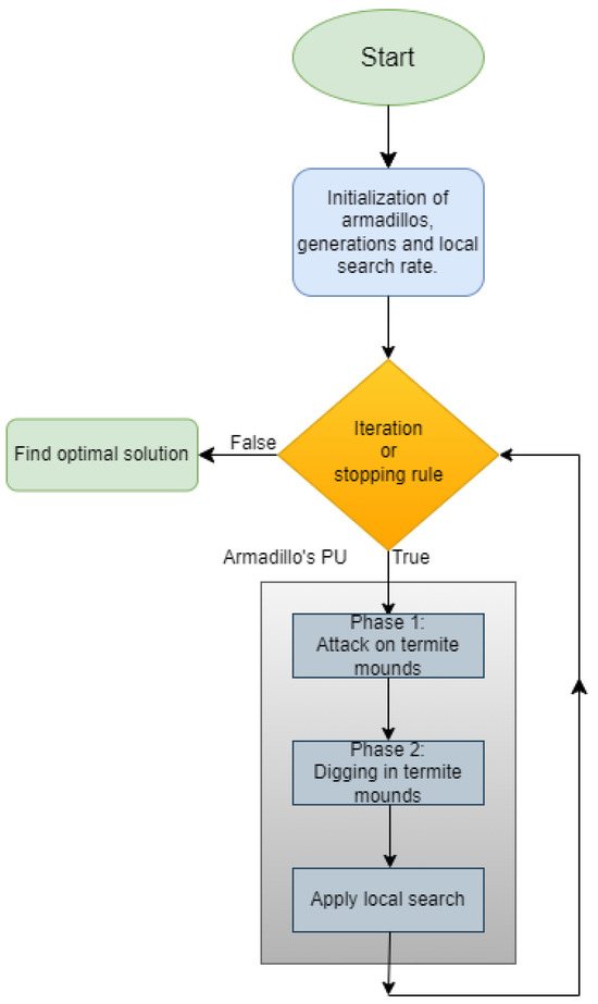
Figure 1.
A schematic representation of the current method.
3. Experiments
This section will begin by detailing the functions that will be used in the experiments. These functions are widespread in the modern global optimization literature and have been used in many research works. Next, the experiments performed using the current method will be presented, and a comparison will be made with methods that are commonly used in the literature of global optimization.
3.1. Experimental Functions
The functions used in the conducted experiments can be found in the related literature [64,65]. The definitions for the functions are listed as follows.
- Bf1 function, defined as:
- Bf2 function, defined as:
- Branin function, defined as: .
- Camel function defined as:
- Easom defined as:
- Exponential function defined as:In the current work, the following values were used for the conducted experiments: .
- Gkls function [66]. The is defined as a function with w local minima, and the dimension of the function was n. For the conducted experiments, the cases of and were used.
- Goldstein and Price function
- Griewank2 function, that has the following definition:
- Griewank10 function defined as:with .
- Hansen function. , .
- Hartman 3 function defined as:with and and
- Hartman 6 function given by:with and and
- Potential function, the well-known Lennard–Jones potential [67] defined as:is adopted as a test case here with .
- Rastrigin function defined as:
- Rosenbrock function.For the conducted experiments, the values were utilized.
- Shekel 7 function.
- Shekel 5 function.
- Shekel 10 function.
- Sinusoidal function defined as:For the current series of experiments the values and were used.
- Test2N function defined as:The function has local minima, and for the conducted experiments, the cases of were used.
- Test30N function defined as:where . This function has local minima, and for the conducted experiments, the cases were used.
3.2. Experimental Results
The software used in the experiments was coded in ANSI-C++. Also, the freely available Optimus optimization environment was incorporated. The software can be downloaded from https://github.com/itsoulos/GlobalOptimus/ (accessed on 14 April 2024). Optimus is entirely written in ANSI-C++ and was prepared using the freely available QT library. All the experiments were executed on an AMD Ryzen 5950X with 128 GB of RAM. The operating system used was Debian Linux. In all experimental tables, the numbers in cells denote average function calls for 30 runs. In each run, a different seed for the random number generator was used. The decimal numbers enclosed in parentheses represent the success rate of the method in finding the global minimum of the corresponding function. If this number does not appear, then the method managed to discover the global minimum in each run. The simulation parameters for the used optimization techniques are listed in Table 1. The values for these parameters were chosen to strike a balance between the expected efficiency of the optimization methods and their speed. All techniques used uniform distribution to initialize the corresponding population.

Table 1.
The experimental values for each parameter used in the conducted experiments.
The results from the conducted experiments are outlined in Table 2. The following applies to this table:
- 1.
- The column PROBLEM denotes the objective problem.
- 2.
- The column GENETIC stands for the average function calls for the Genetic algorithm. The same number of armadillos and chromosomes and particles was used in the experiments conducted to make a fair comparison between the algorithms. Also, the same number of maximum generations and the same stopping criteria were utilized among the different optimization methods.
- 3.
- The column PSO stands for the application of a Particle Swarm Optimization method in the objective problem. The number of particles and the stopping rule in the PSO method are the same as in the proposed method.
- 4.
- The column GWO stands for the application of Gray Wolf Optimizer [68] on the benchmark functions.
- 5.
- The column PROPOSED represents the experimental results for the Gao method with the suggested modifications.
- 6.
- The final row, denoted as SUM, stands for the sum of the function calls and the average success rate for all the used objective functions.
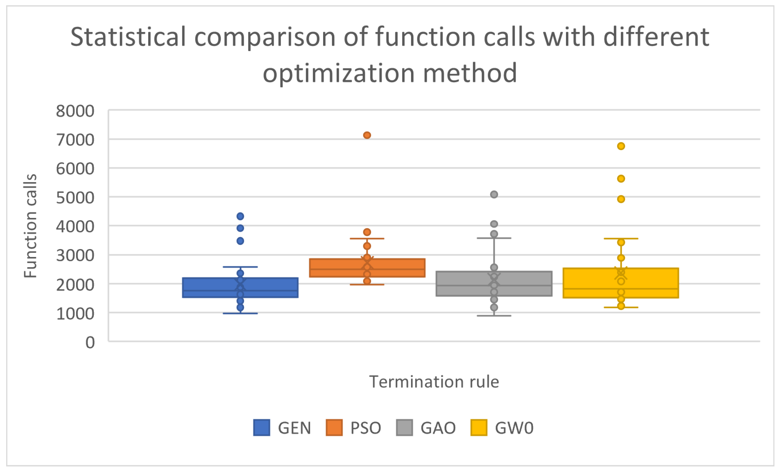
The statistical comparison for the previous experimental results is depicted in Figure 2. The previous experiments and their subsequent statistical processing demonstrate that the proposed method significantly outperforms Particle Swarm Optimization when a comparison is conducted for the average number of function calls since it requires 20% fewer function calls on average to efficiently find the global minimum. In addition, the proposed method appears to have similar efficiency in terms of required function calls to that of the Genetic Algorithm.
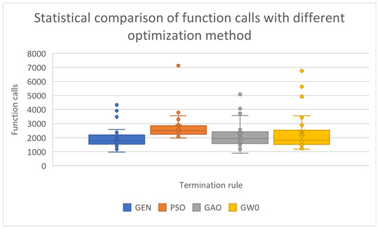
Figure 2.
A statistical comparison using the number of function calls. The test was performed for three different optimization methods.

Table 2.
Experimental results and comparison against other methods. The stopping rule used is the Similarity stopping rule.
Table 2.
Experimental results and comparison against other methods. The stopping rule used is the Similarity stopping rule.
| PROBLEM | Genetic | PSO | GWO | PROPOSED |
|---|---|---|---|---|
| BF1 | 2179 | 2364 (0.97) | 2927 | 2239 |
| BF2 | 1944 | 2269 (0.90) | 2893 | 1864 |
| BRANIN | 1177 | 2088 | 2430 | 1179 |
| CAMEL | 1401 | 2278 | 1533 | 1450 |
| EASOM | 979 | 2172 | 2074 (0.93) | 886 |
| EXP4 | 1474 | 2231 | 1640 | 1499 |
| EXP8 | 1551 | 2256 | 2392 | 1539 |
| EXP16 | 1638 | 2165 | 3564 | 1581 |
| EXP32 | 1704 | 2106 | 5631 | 1567 |
| GKLS250 | 1195 | 2113 | 1407 | 1292 |
| GKLS350 | 1396 (0.87) | 1968 | 1889 | 1510 |
| GOLDSTEIN | 1878 | 2497 | 1820 | 1953 |
| GRIEWANK2 | 2360 (0.87) | 3027 (0.97) | 1914 | 2657 |
| GRIEWANK10 | 3474 (0.87) | 3117 (0.87) | 3427 (0.13) | 4064 (0.97) |
| HANSEN | 1761 (0.97) | 2780 | 2290 (0.60) | 1885 |
| HARTMAN3 | 1404 | 2086 | 1497 | 1448 |
| HARTMAN6 | 1632 | 2213 (0.87) | 1616 (0.53) | 1815 |
| POTENTIAL3 | 2127 | 3557 | 1520 | 1942 |
| POTENTIAL5 | 3919 | 7132 | 2544 | 3722 |
| RASTRIGIN | 2438 (0.97) | 2754 | 1858 | 2411 |
| ROSENBROCK4 | 1841 | 2909 | 4925 | 2690 |
| ROSENBROCK8 | 2570 | 3382 | 5662 | 3573 |
| ROSENBROCK16 | 4331 | 3780 | 6752 | 5085 |
| SHEKEL5 | 1669 (0.97) | 2700 | 1297 (0.53) | 1911 |
| SHEKEL7 | 1696 | 2612 | 1472 (0.60) | 1930 |
| SHEKEL10 | 1758 | 2594 | 1224 (0.57) | 1952 |
| TEST2N4 | 1787 (0.97) | 2285 | 1680 (0.80) | 1840 (0.83) |
| TEST2N5 | 2052 (0.93) | 2368 (0.97) | 1791 (0.73) | 2029 (0.63) |
| TEST2N6 | 2216 (0.73) | 2330 (0.73) | 1710 (0.53) | 2438 (0.80) |
| TEST2N7 | 2520 (0.73) | 2378 (0.63) | 1631 (0.47) | 2567 (0.60) |
| SINU4 | 1514 | 2577 | 1241 (0.70) | 1712 |
| SINU8 | 1697 | 2527 | 1184 (0.83) | 1992 |
| SINU16 | 2279 (0.97) | 2657 | 1296 (0.67) | 2557 |
| TEST30N3 | 1495 | 3302 | 1527 | 1749 |
| TEST30N4 | 1897 | 3817 | 2520 | 2344 |
| SUM | 68,953 (0.97) | 95,391 (0.97) | 82,778 (0.85) | 74,982 (0.97) |
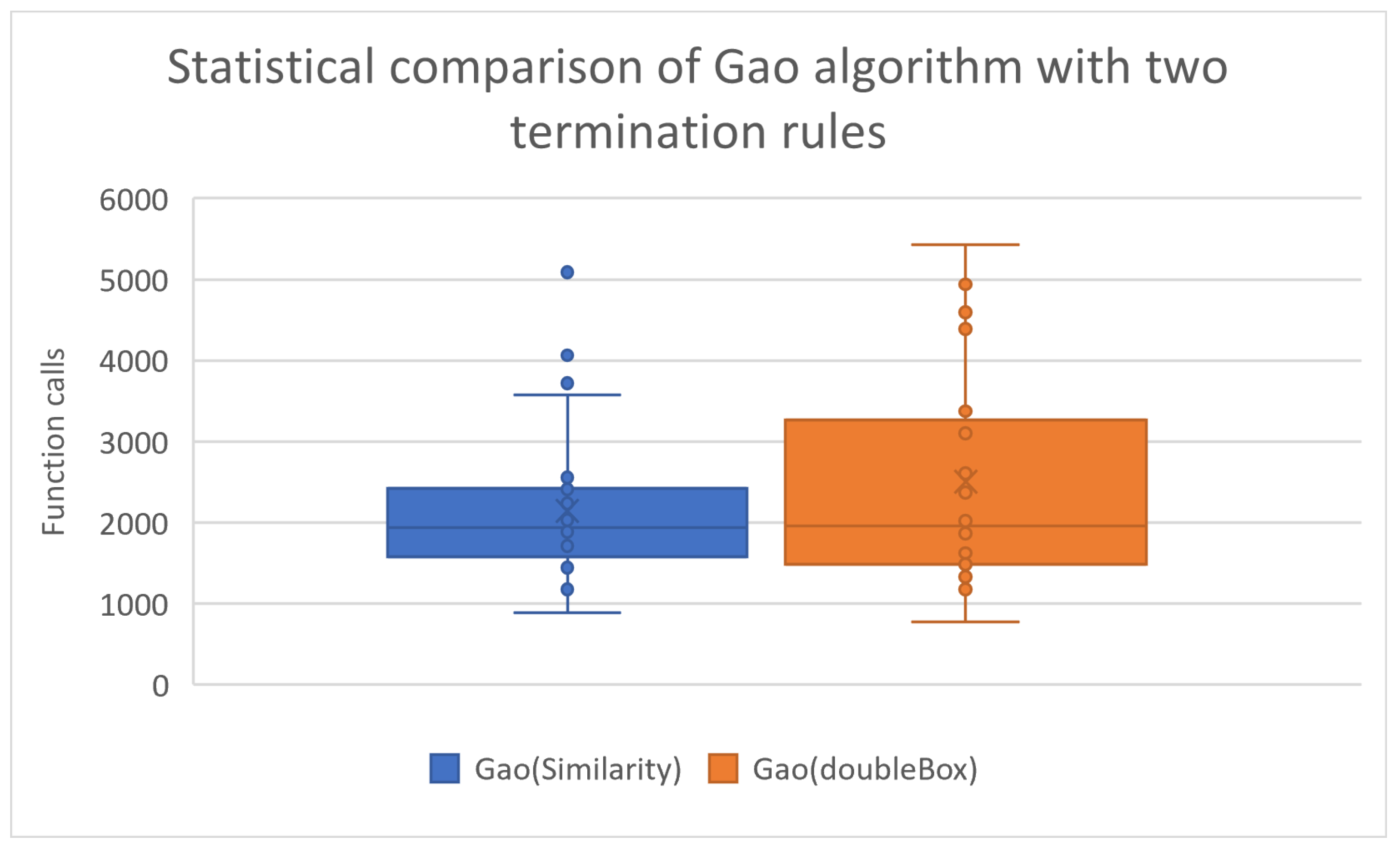
The reliability of the termination techniques was tested with one more experiment, in which both proposed termination rules were used, and the produced results for the benchmark functions are presented in Table 3. Also, the statistical comparison for the experiment is shown graphically in Figure 3.

Table 3.
Average number of function calls for the proposed method using the two suggested termination rules.
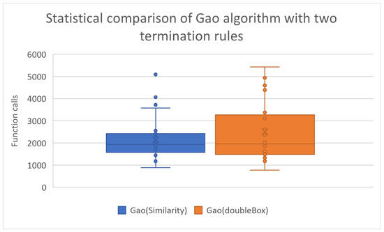
Figure 3.
Comparison of Gao algorithm with two termination rules.
From the statistical processing of the experimental results, one can find that the termination method using the Similarity criterion demands a lower number of function calls than the DoubleBox stopping rule to achieve the goal, which is to effectively find the global minimum. Furthermore, there is no significant difference in the success rate of the two termination techniques, as reflected in the success rate in finding the global minimum, which remains high for both techniques (around 97%).
Moreover, the effect of the application of the local search technique is explored in the experiments shown in Table 4, where the local search rate increases from 0.5% to 5%.

Table 4.
Experimental results using different values for the local search rate and the proposed method.
As expected, the success rate in discovering the global minimum increases as the rate of application of the local minimization technique increases. For the case of the current method, this rate increases from 92% to 97% in the experimental results. This finding demonstrates that if this method is combined with effective local minimization techniques, it can lead to a more efficient finding of the global minimum for the objective function.
Also, to measure the time complexity of the proposed work, the ELP (High Elliptic Function) function was employed with arbitrary dimensions. The function is defined as:
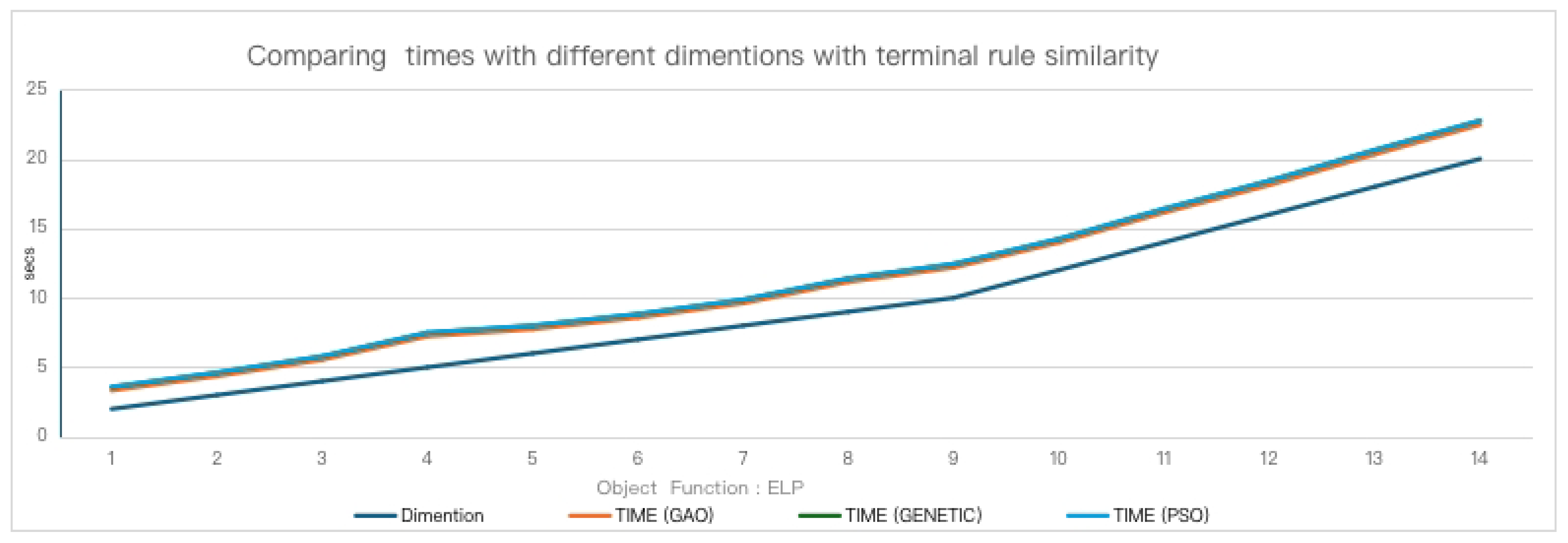
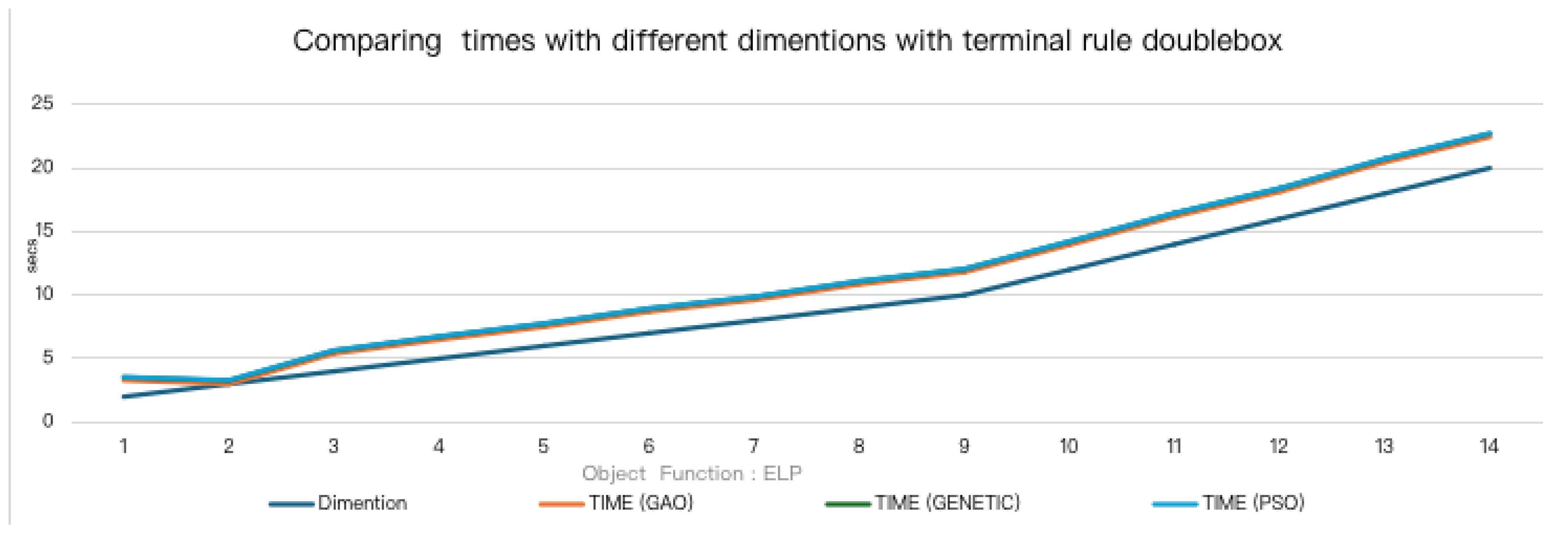
In this test, the dimension of the function (n) increased from 1 to 15, and the average execution time was measured. The results obtained for the similarity termination rule are outlined in Figure 4, and the results for the DoubleBox termination rule are graphically shown in Figure 5.
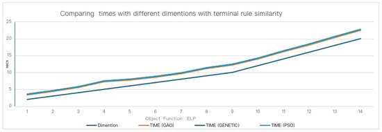
Figure 4.
Representation of the average execution times for the ELP objective function, using the similarity stopping rule.
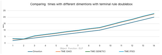
Figure 5.
Representation of the average execution times for the ELP objective function, using the DoubleBox stopping rule.
As expected, the execution time increases as the dimensions of the function increase, but there are no significant differences between the execution times of the three optimization methods.
Furthermore, as a practical application, consider the training of an artificial neural network for classification or data fitting problems [69,70]. Neural networks are non-linear parametric tools with many applications in real-world problems [71,72,73]. Neural networks can be defined as functions . The vector represents the input pattern, while the vector represents the weight vector of the neural network that should be estimated. Optimization methods can be used to estimate the set of weights by minimizing the following equation:
The quantity of Equation (3) was minimized using the mentioned algorithm of this work for the BK dataset [74], which is used to estimate the points in a basketball game. The average test error using the four methods presented in this article is shown graphically in Figure 6. To validate the results, the well-known ten-fold cross method was applied. The current work has the same performance as the PSO algorithm and significantly outperforms the Genetic algorithm.
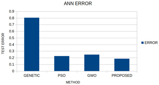
Figure 6.
Comparison of test error between the mentioned global optimization algorithms for the BK dataset.
4. Conclusions
Two modifications for the Giant-Armadillo Optimization method were suggested in this article. These modifications aimed to improve the efficiency and the speed of the underlying global optimization algorithm. The first modification suggested the periodic application of a local optimization procedure to randomly selected armadillos from the current population. The second modification utilized some stopping rules from the recent bibliography to stop the more efficient optimization method and to avoid unnecessary iterations when the global minimum was already discovered. The modified global optimization method was tested against two other global optimization methods from the relevant literature and, more specifically, an implementation of the Genetic Algorithm and a Particle Swarm Optimization variant on a series of well-known test functions. To make a fair comparison between these methods, the same number of test solutions (armadillo or chromosomes) and the same termination rule were used. The present technique, after comparing the experimental results, clearly outperforms particle optimization and has a similar behavior to that of the genetic algorithm. Also, after a series of experiments, it was shown that the Similarity termination rule outperforms the DoubleBox termination rule in terms of function calls without reducing the effectiveness of the proposed method in the task of locating the global minimum.
Since the experimental results have been shown to be extremely promising, further efforts can be made to develop the technique in various fields. For example, an extension could be to develop a termination rule that exploits the particularities of the particular global optimization technique. Among the future extensions of the application may be the use of parallel computing techniques to speed up the optimization process, such as the incorporation of the MPI [75] or the OpenMP library [76]. For example, in this direction, it could be investigated to parallelize the technique in a similar way as genetic algorithms using islands [77,78].
Author Contributions
G.K., V.C. and I.G.T. conceived of the idea and the methodology, and G.K. and V.C. implemented the corresponding software. G.K. conducted the experiments, employing objective functions as test cases, and provided the comparative experiments. I.G.T. performed the necessary statistical tests. All authors have read and agreed to the published version of the manuscript.
Funding
This research has been financed by the European Union: Next Generation EU through the Program Greece 2.0 National Recovery and Resilience Plan, under the call RESEARCH–CREATE–INNOVATE, project name “iCREW: Intelligent small craft simulator for advanced crew training using Virtual Reality techniques” (project code: TAEDK-06195).
Institutional Review Board Statement
Not applicable.
Informed Consent Statement
Not applicable.
Data Availability Statement
The original contributions presented in the study are included in the article, further inquiries can be directed to the corresponding author.
Conflicts of Interest
The authors declare no conflicts of interest.
References
- Rothlauf, F.; Rothlauf, F. Optimization problems. In Design of Modern Heuristics: Principles and Application; Springer: Berlin/Heidelberg, Germany, 2011; pp. 7–44. [Google Scholar]
- Horst, R.; Pardalos, P.M.; Van Thoai, N. Introduction to Global Optimization; Springer Science & Business Media: Berlin/Heidelberg, Germany, 2000. [Google Scholar]
- Weise, T. Global optimization algorithms-theory and application. Self-Publ. Thomas Weise 2009, 361, 153. [Google Scholar]
- Ovelade, O.N.; Ezugwu, A.E. Ebola Optimization Search Algorithm: A new nature-inspired metaheuristic algorithm for global optimization problems. In Proceedings of the 2021 International Conference on Electrical, Computer and Energy Technologies (ICECET), Cape Town, South Africa, 9–10 December 2021; IEEE: New York, NY, USA, 2021; pp. 1–10. [Google Scholar]
- Deb, K.; Sindhya, K.; Hakanen, J. Multi-objective optimization. In Decision Sciences; CRC Press: Boca Raton, FL, USA, 2016; pp. 161–200. [Google Scholar]
- Liberti, L.; Kucherenko, S. Comparison of deterministic and stochastic approaches to global optimization. Int. Trans. Oper. Res. 2005, 12, 263–285. [Google Scholar] [CrossRef]
- Casado, L.G.; García, I.; Csendes, T. A new multisection technique in interval methods for global optimization. Computing 2000, 65, 263–269. [Google Scholar] [CrossRef]
- Zhang, X.; Liu, S. Interval algorithm for global numerical optimization. Eng. Optim. 2008, 40, 849–868. [Google Scholar] [CrossRef]
- Price, W. Global optimization by controlled random search. J. Optim. Theory Appl. 1983, 40, 333–348. [Google Scholar] [CrossRef]
- Křivỳ, I.; Tvrdík, J. The controlled random search algorithm in optimizing regression models. Comput. Stat. Data Anal. 1995, 20, 229–234. [Google Scholar] [CrossRef]
- Ali, M.M.; Törn, A.; Viitanen, S. A numerical comparison of some modified controlled random search algorithms. J. Glob. Optim. 1997, 11, 377–385. [Google Scholar] [CrossRef]
- Aarts, E.; Korst, J.; Michiels, W. Simulated annealing. In Search Methodologies: Introductory Tutorials in Optimization and Decision Support Techniques; Springer: Berlin/Heidelberg, Germany, 2005; pp. 187–210. [Google Scholar]
- Nikolaev, A.G.; Jacobson, S.H. Simulated annealing. In Handbook of Metaheuristics; Springer: Berlin/Heidelberg, Germany, 2010; pp. 1–39. [Google Scholar]
- Rinnooy Kan, A.; Timmer, G. Stochastic global optimization methods part II: Multi level methods. Math. Program. 1987, 39, 57–78. [Google Scholar] [CrossRef]
- Ali, M.M.; Storey, C. Topographical multilevel single linkage. J. Glob. Optim. 1994, 5, 349–358. [Google Scholar] [CrossRef]
- Tsoulos, I.G.; Lagaris, I.E. MinFinder: Locating all the local minima of a function. Comput. Phys. Commun. 2006, 174, 166–179. [Google Scholar] [CrossRef]
- Pardalos, P.M.; Romeijn, H.E.; Tuy, H. Recent developments and trends in global optimization. J. Comput. Appl. Math. 2000, 124, 209–228. [Google Scholar] [CrossRef]
- Fouskakis, D.; Draper, D. Stochastic optimization: A review. Int. Stat. Rev. 2002, 70, 315–349. [Google Scholar] [CrossRef]
- Rocki, K.; Suda, R. An efficient GPU implementation of a multi-start TSP solver for large problem instances. In Proceedings of the 14th Annual Conference Companion on Genetic and Evolutionary Computation, Philadelphia, PA, USA, 7–11 July 2012; pp. 1441–1442. [Google Scholar]
- Van Luong, T.; Melab, N.; Talbi, E.G. GPU-based multi-start local search algorithms. In Proceedings of the Learning and Intelligent Optimization: 5th International Conference, LION 5, Rome, Italy, 17–21 January 2011; Selected Papers 5. Springer: Berlin/Heidelberg, Germany, 2011; pp. 321–335. [Google Scholar]
- Bartz-Beielstein, T.; Branke, J.; Mehnen, J.; Mersmann, O. Evolutionary algorithms. Wiley Interdiscip. Rev. Data Min. Knowl. Discov. 2014, 4, 178–195. [Google Scholar] [CrossRef]
- Simon, D. Evolutionary Optimization Algorithms; John Wiley & Sons: Hoboken, NJ, USA, 2013. [Google Scholar]
- Blum, C. Ant colony optimization: Introduction and recent trends. Phys. Life Rev. 2005, 2, 353–373. [Google Scholar] [CrossRef]
- Dorigo, M.; Blum, C. Ant colony optimization theory: A survey. Theor. Comput. Sci. 2005, 344, 243–278. [Google Scholar] [CrossRef]
- Haldurai, L.; Madhubala, T.; Rajalakshmi, R. A study on genetic algorithm and its applications. Int. J. Comput. Sci. Eng. 2016, 4, 139. [Google Scholar]
- Jamwal, P.K.; Abdikenov, B.; Hussain, S. Evolutionary optimization using equitable fuzzy sorting genetic algorithm (EFSGA). IEEE Access 2019, 7, 8111–8126. [Google Scholar] [CrossRef]
- Wang, Z.; Sobey, A. A comparative review between Genetic Algorithm use in composite optimisation and the state-of-the-art in evolutionary computation. Compos. Struct. 2020, 233, 111739. [Google Scholar] [CrossRef]
- Eberhart, R.; Kennedy, J. Particle swarm optimization. In Proceedings of the IEEE International Conference on Neural Networks, Perth, Australia, 27 November–1 December 1995; Citeseer: Princeton, NJ, USA, 1995; Volume 4, pp. 1942–1948. [Google Scholar]
- Wang, D.; Tan, D.; Liu, L. Particle swarm optimization algorithm: An overview. Soft Comput. 2018, 22, 387–408. [Google Scholar] [CrossRef]
- Price, K.V. Differential evolution. In Handbook of Optimization: From Classical to Modern Approach; Springer: Berlin/Heidelberg, Germany, 2013; pp. 187–214. [Google Scholar]
- Pant, M.; Zaheer, H.; Garcia-Hernandez, L.; Abraham, A. Differential Evolution: A review of more than two decades of research. Eng. Appl. Artif. Intell. 2020, 90, 103479. [Google Scholar]
- Asselmeyer, T.; Ebeling, W.; Rosé, H. Evolutionary strategies of optimization. Phys. Rev. 1997, 56, 1171. [Google Scholar] [CrossRef]
- Arnold, D.V. Noisy Optimization with Evolution Strategies; Springer Science & Business Media: Berlin/Heidelberg, Germany, 2002; Volume 8. [Google Scholar]
- Yao, X.; Liu, Y.; Lin, G. Evolutionary programming made faster. IEEE Trans. Evol. Comput. 1999, 3, 82–102. [Google Scholar]
- Stephenson, M.; O’Reilly, U.M.; Martin, M.C.; Amarasinghe, S. Genetic programming applied to compiler heuristic optimization. In Proceedings of the European Conference on Genetic Programming, Essex, UK, 14–16 April 2003; Springer: Berlin/Heidelberg, Germany, 2003; pp. 238–253. [Google Scholar]
- Banga, J.R. Optimization in computational systems biology. BMC Syst. Biol. 2008, 2, 47. [Google Scholar] [CrossRef]
- Beites, T.; Mendes, M.V. Chassis optimization as a cornerstone for the application of synthetic biology based strategies in microbial secondary metabolism. Front. Microbiol. 2015, 6, 159095. [Google Scholar] [CrossRef]
- Hartmann, A.K.; Rieger, H. Optimization Algorithms in Physics; Citeseer: Princeton, NJ, USA, 2002. [Google Scholar]
- Hanuka, A.; Huang, X.; Shtalenkova, J.; Kennedy, D.; Edelen, A.; Zhang, Z.; Lalchand, V.; Ratner, D.; Duris, J. Physics model-informed Gaussian process for online optimization of particle accelerators. Phys. Rev. Accel. Beams 2021, 24, 072802. [Google Scholar] [CrossRef]
- Ferreira, S.L.; Lemos, V.A.; de Carvalho, V.S.; da Silva, E.G.; Queiroz, A.F.; Felix, C.S.; da Silva, D.L.; Dourado, G.B.; Oliveira, R.V. Multivariate optimization techniques in analytical chemistry-an overview. Microchem. J. 2018, 140, 176–182. [Google Scholar] [CrossRef]
- Bechikh, S.; Chaabani, A.; Said, L.B. An efficient chemical reaction optimization algorithm for multiobjective optimization. IEEE Trans. Cybern. 2014, 45, 2051–2064. [Google Scholar] [CrossRef] [PubMed]
- Filip, M.; Zoubek, T.; Bumbalek, R.; Cerny, P.; Batista, C.E.; Olsan, P.; Bartos, P.; Kriz, P.; Xiao, M.; Dolan, A.; et al. Advanced computational methods for agriculture machinery movement optimization with applications in sugarcane production. Agriculture 2020, 10, 434. [Google Scholar] [CrossRef]
- Zhang, D.; Guo, P. Integrated agriculture water management optimization model for water saving potential analysis. Agric. Water Manag. 2016, 170, 5–19. [Google Scholar] [CrossRef]
- Intriligator, M.D. Mathematical Optimization and Economic Theory; SIAM: Philadelphia, PA, USA, 2002. [Google Scholar]
- Dixit, A.K. Optimization in Economic Theory; Oxford University Press: Oxford, MA, USA, 1990. [Google Scholar]
- Abdel-Basset, M.; Abdel-Fatah, L.; Sangaiah, A.K. Metaheuristic algorithms: A comprehensive review. In Computational Intelligence for Multimedia Big Data on the Cloud with Engineering Applications; Academic Press: Cambridge, MA, USA, 2018; pp. 185–231. [Google Scholar]
- Ezugwu, A.E.; Shukla, A.K.; Nath, R.; Akinyelu, A.A.; Agushaka, J.O.; Chiroma, H.; Muhuri, P.K. Metaheuristics: A comprehensive overview and classification along with bibliometric analysis. Artif. Intell. Rev. 2021, 54, 4237–4316. [Google Scholar] [CrossRef]
- Montoya, O.D.; Molina-Cabrera, A.; Gil-González, W. A Possible Classification for Metaheuristic Optimization Algorithms in Engineering and Science. Ingeniería 2022, 27, e19815. [Google Scholar]
- Bhattacharyya, T.; Chatterjee, B.; Singh, P.K.; Yoon, J.H.; Geem, Z.W.; Sarkar, R. Mayfly in harmony: A new hybrid meta-heuristic feature selection algorithm. IEEE Access 2020, 8, 195929–195945. [Google Scholar] [CrossRef]
- Alsayyed, O.; Hamadneh, T.; Al-Tarawneh, H.; Alqudah, M.; Gochhait, S.; Leonova, I.; Malik, O.P.; Dehghani, M. Giant Armadillo Optimization: A New Bio-Inspired Metaheuristic Algorithm for Solving Optimization Problems. Biomimetics 2023, 8, 619. [Google Scholar] [CrossRef] [PubMed]
- Desbiez, A.; Kluyber, D.; Massocato, G.; Attias, N. Methods for the characterization of activity patterns in elusive species: The giant armadillo in the Brazilian Pantanal. J. Zool. 2021, 315, 301–312. [Google Scholar] [CrossRef]
- Owaid, S.R.; Zhuravskyi, Y.; Lytvynenko, O.; Veretnov, A.; Sokolovskyi, D.; Plekhova, G.; Hrinkov, V.; Pluhina, T.; Neronov, S.; Dovbenko, O. Development of a method of increasing the efficiency of decision-making in organizational and technical systems. East.-Eur. J. Enterp. Technol. 2024, 1, 127. [Google Scholar] [CrossRef]
- Basheer, I.A.; Hajmeer, M. Artificial neural networks: Fundamentals, computing, design, and application. J. Microbiol. Methods 2000, 43, 3–31. [Google Scholar] [CrossRef] [PubMed]
- Zou, J.; Han, Y.; So, S.S. Overview of artificial neural networks. In Artificial Neural Networks: Methods and Applications; Springer: Berlin/Heidelberg, Germany, 2009; pp. 14–22. [Google Scholar]
- Kennedy, J. Swarm intelligence. In Handbook of Nature-Inspired and Innovative Computing: Integrating Classical Models with Emerging Technologies; Springer: Boston, MA, USA, 2006; pp. 187–219. [Google Scholar]
- Macedo, M.; Siqueira, H.; Figueiredo, E.; Santana, C.; Lira, R.C.; Gokhale, A.; Bastos-Filho, C. Overview on binary optimization using swarm-inspired algorithms. IEEE Access 2021, 9, 149814–149858. [Google Scholar] [CrossRef]
- Dhawan, S.; Gupta, R.; Rana, A.; Sharma, S. Various swarm optimization algorithms: Review, challenges, and opportunities. In Soft Computing for Intelligent Systems: Proceedings of ICSCIS 2020; Springer: Berlin/Heidelberg, Germany, 2021; pp. 291–301. [Google Scholar]
- Fletcher, R. A new approach to variable metric algorithms. Comput. J. 1970, 13, 317–322. [Google Scholar] [CrossRef]
- Yuan, Y.x. A new stepsize for the steepest descent method. J. Comput. Math. 2006, 24, 149–156. [Google Scholar]
- Zhu, C.; Byrd, R.H.; Lu, P.; Nocedal, J. Algorithm 778: L-BFGS-B: Fortran subroutines for large-scale bound-constrained optimization. ACM Trans. Math. Softw. (TOMS) 1997, 23, 550–560. [Google Scholar] [CrossRef]
- Powell, M. A tolerant algorithm for linearly constrained optimization calculations. Math. Program. 1989, 45, 547–566. [Google Scholar] [CrossRef]
- Tsoulos, I.G. Modifications of real code genetic algorithm for global optimization. Appl. Math. Comput. 2008, 203, 598–607. [Google Scholar] [CrossRef]
- Charilogis, V.; Tsoulos, I.G. Toward an Ideal Particle Swarm Optimizer for Multidimensional Functions. Information 2022, 13, 217. [Google Scholar] [CrossRef]
- Ali, M.M.; Khompatraporn, C.; Zabinsky, Z.B. A numerical evaluation of several stochastic algorithms on selected continuous global optimization test problems. J. Glob. Optim. 2005, 31, 635–672. [Google Scholar] [CrossRef]
- Floudas, C.A.; Pardalos, P.M.; Adjiman, C.; Esposito, W.R.; Gümüs, Z.H.; Harding, S.T.; Klepeis, J.L.; Meyer, C.A.; Schweiger, C.A. Handbook of Test Problems in Local and Global Optimization; Springer Science & Business Media: Berlin/Heidelberg, Germany, 2013; Volume 33. [Google Scholar]
- Gaviano, M.; Kvasov, D.E.; Lera, D.; Sergeyev, Y.D. Algorithm 829: Software for generation of classes of test functions with known local and global minima for global optimization. ACM Trans. Math. Softw. (TOMS) 2003, 29, 469–480. [Google Scholar] [CrossRef]
- Jones, J.E. On the determination of molecular fields.—II. From the equation of state of a gas. Proc. R. Soc. Lond. Ser. Contain. Pap. Math. Phys. Character 1924, 106, 463–477. [Google Scholar]
- Mirjalili, S.; Mirjalili, S.M.; Lewis, A. Grey Wolf Optimizer. Adv. Eng. Softw. 2014, 69, 46–61. [Google Scholar] [CrossRef]
- Bishop, C.M. Neural Networks for Pattern Recognition; Oxford University Press: Oxford, UK, 1995. [Google Scholar]
- Cybenko, G. Approximation by superpositions of a sigmoidal function. Math. Control. Signals Syst. 1989, 2, 303–314. [Google Scholar] [CrossRef]
- Topuz, A. Predicting moisture content of agricultural products using artificial neural networks. Adv. Eng. Softw. 2010, 41, 464–470. [Google Scholar] [CrossRef]
- Boughrara, H.; Chtourou, M.; Ben Amar, C.; Chen, L. Facial expression recognition based on a mlp neural network using constructive training algorithm. Multimed. Tools Appl. 2016, 75, 709–731. [Google Scholar] [CrossRef]
- Carleo, G.; Troyer, M. Solving the quantum many-body problem with artificial neural networks. Science 2017, 355, 602–606. [Google Scholar] [CrossRef]
- Simonoff, J.S. Smoothing Methods in Statistics; Springer Science & Business Media: Berlin/Heidelberg, Germany, 2012. [Google Scholar]
- Gropp, W.; Lusk, E.; Doss, N.; Skjellum, A. A high-performance, portable implementation of the MPI message passing interface standard. Parallel Comput. 1996, 22, 789–828. [Google Scholar] [CrossRef]
- Chandra, R. Parallel Programming in OpenMP; Morgan Kaufmann: Cambridge, MA, USA, 2001. [Google Scholar]
- Li, C.C.; Lin, C.H.; Liu, J.C. Parallel genetic algorithms on the graphics processing units using island model and simulated annealing. Adv. Mech. Eng. 2017, 9, 1687814017707413. [Google Scholar] [CrossRef]
- da Silveira, L.A.; Soncco-Álvarez, J.L.; de Lima, T.A.; Ayala-Rincón, M. Parallel island model genetic algorithms applied in NP-hard problems. In Proceedings of the 2019 IEEE Congress on Evolutionary Computation (CEC), Wellington, New Zealand, 10–13 June 2019; IEEE: New York, NY, USA, 2019; pp. 3262–3269. [Google Scholar]
Disclaimer/Publisher’s Note: The statements, opinions and data contained in all publications are solely those of the individual author(s) and contributor(s) and not of MDPI and/or the editor(s). MDPI and/or the editor(s) disclaim responsibility for any injury to people or property resulting from any ideas, methods, instructions or products referred to in the content. |
© 2024 by the authors. Licensee MDPI, Basel, Switzerland. This article is an open access article distributed under the terms and conditions of the Creative Commons Attribution (CC BY) license (https://creativecommons.org/licenses/by/4.0/).


