Theoretical Contributions to Three Generalized Versions of the Celebioglu–Cuadras Copula

Abstract

Copulas are probabilistic functions that are being used more and more frequently to describe, examine, and model the interdependence of continuous random variables. Among the numerous proposed copulas, renewed interest has recently been shown in the so-called Celebioglu–Cuadras copula. It is mainly because of its simplicity, exploitable dependence properties, and potential for applicability. In this article, we contribute to the development of this copula by proposing three generalized versions of it, each involving three tuning parameters. The main results are theoretical: they consist of determining wide and manageable intervals of admissible values for the involved parameters. The proofs are mainly based on limit, differentiation, and factorization techniques as well as mathematical inequalities. Some of the configuration parameters are new in the literature, and original phenomena are revealed. Subsequently, the basic properties of the proposed copulas are studied, such as symmetry, quadrant dependence, various expansions, concordance ordering, tail dependences, medial correlation, and Spearman correlation. Detailed examples, numerical tables, and graphics are used to support the theory.

1. Introduction

In the fields of statistics, probability, informatics, engineering, insurance, physics, hydrology, medicine, astronomy, etc., copulas are prevalent. They are crucial for outlining, investigating, and modeling the interconnectedness of the involved continuous random variables. When only two continuous random variables are considered, which is the case in many applications, two-dimensional copulas are required. A two-dimensional copula can be defined as a cumulative distribution function (CDF) with uniform marginal distributions on the unit square $I={[0,1]}^2$. In the absolutely continuous case, a precise definition is given below.

Definition 1.

The function $C:I\to [0,1]$ is an (absolutely continuous) two-dimensional copula if and only if

(i) 

we have $C(x,0)=C(0,y)=0$ for any $(x,y)\in I$;

(ii) 

we have $C(x,1)=x$ and $C(1,y)=y$ for any $(x,y)\in I$;

(iii) 

we have

$${\displaystyle \frac{{\partial }^2}{\partial x\partial y}C(x,y)\ge 0}$$

for any $(x,y)\in I$.

Numerous two-dimensional copulas have been investigated in the literature. Exhaustive lists can be found in [1,2,3,4]. The Ali–Mikhail–Haq (AMH), Clayton, Farlie–Gumbel–Morgenstern (FGM), Frank, Fréchet, Galambos, Gumbel–Barnett (GB), Gumbel–Hougaard, Hüsler–Reiss, Joe, Marshall–Olkin, Plackett, and Raftery copulas are among the most famous. They often depend on one or more parameters that confer interesting levels of dependence and flexibility. Hence, classical copulas have been involved in numerous applications. See, for instance, [5,6,7,8]. Moreover, with the tremendous developments in computer calculation, the subject of the copula is more interesting than ever for modern theoretical and practical problems. Recent contributions on this topic can be found in [9,10,11,12,13,14,15,16].

For the purposes of this paper, a retrospective on the GB copula is necessary. To begin, the GB copula can be presented as

$$C(x,y;a)=xyexp\left[a(logx)(logy)\right],(x,y)\in I,$$

with $a\in [-1,0]$. It has the particularity of being one of the simplest Archimedean copula, covering the independence copula: $C(x,y;0)=xy$, and being well adapted to model various negative-type dependence. See, for instance, [4]. Among the most recent developments in the GB copula, the authors in [17,18] proposed a modified version demonstrating a broader range of dependence. This modified GB copula, called the Celebioglu–Cuadras (CC) copula, is indicated as

$$C(x,y;a)=xyexp\left[a(1-x)(1-y)\right],(x,y)\in I,$$

with $a\in [-1,1]$. In addition to being flexible in the dependence sense, the CC copula has a simple mathematical form, covers the independence copula, and has manageable properties, including negative and positive-type dependence. It was recently mentioned in diverse research articles, often as a member of general families of copulas. See, for instance, Ref. [19] (Example 2.2), [20] (Example 2), [21] (Example 5), and [22] (Example 2). However, to the best of our knowledge, despite the immediate advantages of this copula, there is not much attention given to it.

In this paper, we provide theoretical contributions to the CC copula by proposing three logical three-parameter generalizations of it. Our methodology follows the power generalization schemes proposed in [23], where three-parameter-power-type generalizations of the FGM copula are discussed. To be more precise, our proposed copulas are of the following forms:

Form 1:

$C_1(x,y;\theta )=xyexp\left[a(1-x^b)(1-y^c)\right]$,

Form 2:

$C_2(x,y;\theta )=xyexp\left[a{(1-x)}^b{(1-y)}^c\right]$,

Form 3:

$C_3(x,y;\theta )=xyexp\left[a(1-x^b){(1-y)}^c\right]$,

where $\theta =(a,b,c)\in {\mathbb{R}}^3$.

Some of these generalized forms have been sketched in [19,22], but only for specific values of a, b, and c. To the best of our knowledge, no global studies exist, and this paper aims to fill this gap. Thus, the main challenge of this study is to determine wide and manageable admissible domains of values for a, b, and c so that copulas of these forms remain mathematically valid. Among the results, we show that negative values for b and c are allowed, which goes beyond previous research and opens up new modeling possibilities. Detailed examples are discussed, and graphics illustrate the theoretical findings. For the three proposed copulas, we determine the expressions of the corresponding copula densities and survival copulas. We explore some of their key properties, such as symmetry, quadrant dependence, various expansions, concordance ordering, tail dependences, medial correlation, and Spearman correlation.

The organization of the paper is composed of the following sections: Section 2 presents the first generalization of the CC copula as well as its properties. Section 3 and Section 4 are analogous to Section 2 but for other generalizations of the CC copula (of Forms 2 and 3, respectively). The paper ends with a conclusion in Section 5.

2. Generalized CC Copula

2.1. Presentation and Result

The first proposed generalized CC copula is presented in the proposition below.

Proposition 1.

Let $\theta =(a,b,c)\in {\mathbb{R}}^3$. We consider the function $C_1(·;\theta ):I\to [0,1]$ defined by

$$\begin{array}{c}\hfill C_1(x,y;\theta )=xyexp\left[a(1-x^b)(1-y^c)\right],(x,y)\in I.\end{array}$$

(1)

Then, $C_1(x,y;\theta )$ is a copula for the following parameter configurations (non-overlapping):

Configuration 1:

$a\ge 0$, $b>0$, $c>0$, $ab\le 1$, and $ac\le 1$.

Configuration 2:

$a<0$, $b>0$, $c>0$, and $abc\ge -1$.

Configuration 3:

$a<0$, $b<0$, $c<0$, $ab\ge 1$, $ac\ge 1$, and $b+(1-ab)c+bc\le 0$.

Proof. 

The proof is based on Definition 1 and limit, differentiation, well-chosen factorization techniques, and inequalities. Let us distinguish the three different parameter configurations.

Configuration 1:

We recall that $a\ge 0$, $b>0$, $c>0$, $ab\le 1$, and $ac\le 1$.

(i) 

For any $x\in [0,1]$, we have $C_1(x,0;\theta )=x\times 0\times exp\left[a(1-x^b)(1-0^c)\right]=0$, and, similarly, for any $y\in [0,1]$, $C_1(0,y;\theta )=0$.

(ii) 

For any $x\in [0,1]$, we have $C_1(x,1;\theta )=x\times 1\times exp\left[a(1-x^b)(1-1^c)\right]=x$, and, similarly, for any $y\in [0,1]$, $C_1(1,y;\theta )=y$.

(iii) 

For any $(x,y)\in I$, using standard differentiation techniques and appropriate factorizations, we have

$$\begin{array}{cc}\hfill & \frac{{\partial }^2}{\partial x\partial y}{C}_1(x,y;\theta )=exp\left[a(1-x^b)(1-x^c)\right]\times \hfill \\ \hfill & \left[a^{2}bc{x}^b{y}^c(1-x^b)(1-y^c)+(ab+ac+abc)x^b{y}^c-ab{x}^b-ac{y}^c+1\right]\hfill \\ \hfill & =exp\left[a(1-x^b)(1-x^c)\right]\left[f(x,y;\theta )+g(x,y;\theta )+h(x,y;\theta )\right],\hfill \end{array}$$

(2)

where

$$f(x,y;\theta )=a^{2}bc{x}^b{y}^c(1-x^b)(1-y^c),g(x,y;\theta )=(1-ab{x}^b)(1-ac{y}^c)$$

and

$$h(x,y;\theta )=a\left(b+(1-ab)c+bc\right)x^b{y}^c.$$

Let us show that these functions are all positive (the exponential term in Equation (2) is always positive). Since $(x,y)\in I$, $b>0$, and $c>0$, it is obvious that $f(x,y;\theta )\ge 0$. Since $(x,y)\in I$, $ab\le 1$, and $ac\le 1$, we immediately have $g(x,y;\theta )\ge 0$. Since $(x,y)\in I$, $b>0$, $c>0$, and $ab\le 1$, we have $b+(1-ab)c+bc\ge 0$, and since $a\ge 0$, we have $h(x,y;\theta )\ge 0$. As a result, for Configuration 1, we have

$$\frac{{\partial }^2}{\partial x\partial y}{C}_1(x,y;\theta )\ge 0.$$

This ends the first portion of the proof.

Configuration 2:

We recall that $a<0$, $b>0$, $c>0$, and $abc\ge -1$.

(i) and (ii)

These points are similar to (i) and (ii) of Configuration 1.

(iii) 

For any $(x,y)\in I$, by considering the basis of Equation (2), but with a different decomposition more appropriate to the situation, we have

$$\begin{array}{cc}\hfill & \frac{{\partial }^2}{\partial x\partial y}{C}_1(x,y;\theta )=exp\left[a(1-x^b)(1-x^c)\right]\times \hfill \\ \hfill & \left[a^{2}bc{x}^b{y}^c(1-x^b)(1-y^c)+(ab+ac+abc)x^b{y}^c-ab{x}^b-ac{y}^c+1\right]\hfill \\ \hfill & =exp\left[a(1-x^b)(1-x^c)\right]\left[f(x,y;\theta )+g(x,y;\theta )+h(x,y;\theta )\right],\hfill \end{array}$$

where

$$f(x,y;\theta )=a^{2}bc{x}^b{y}^c(1-x^b)(1-y^c),g(x,y;\theta )=-ac(1-x^b)y^c$$

and

$$h(x,y;\theta )=1+ab{x}^b\left((c+1)y^c-1\right).$$

Let us prove that these functions are positive. Since $(x,y)\in I$, $b>0$, and $c>0$, we immediately have $f(x,y;\theta )\ge 0$. Since $(x,y)\in I$, $a<0$, $b>0$, and $c>0$, we have $g(x,y;\theta )\ge 0$. Since $(x,y)\in I$ and $c>0$, we have $(c+1)y^c-1\le (c+1)-1=c$. Hence, since $a<0$, $b>0$, $c>0$, and $abc\ge -1$, we obtain

$$h(x,y;\theta )\ge 1+abc{x}^b\ge 1-x^b\ge 0.$$

As a result, for Configuration 2, we have

$$\frac{{\partial }^2}{\partial x\partial y}{C}_1(x,y;\theta )\ge 0.$$

This ends the second portion of the proof.

Configuration 3:

We recall that $a<0$, $b<0$, $c<0$, $ab\ge 1$, $ac\ge 1$, and $b+(1-ab)c+bc\le 0$.

(i) 

For any $x\in [0,1]$, since $a<0$, $b<0$, and $c<0$, assumptions that are crucial here, we have $C_1(x,0;\theta )={lim}_{y\to 0}xyexp\left[a(1-x^b)(1-y^c)\right]=0\times 0=0$ (it is ∞ if $c>0$, hence the importance to have $c<0$), and, similarly, for any $y\in [0,1]$, $C_1(0,y;\theta )={lim}_{x\to 0}xyexp\left[a(1-x^b)(1-y^c)\right]=0\times 0=0$ (it is ∞ if $b>0$, hence the importance to have $b<0$).

(ii) 

For any $x\in [0,1]$, we have $C_1(x,1;\theta )=x\times 1\times exp\left[a(1-x^b)(1-1^c)\right]=x$, and, similarly, for any $y\in [0,1]$, $C_1(1,y;\theta )=y$.

(iii) 

For any $(x,y)\in I$, based on Equation (2), we have

$$\begin{array}{cc}\hfill & \frac{{\partial }^2}{\partial x\partial y}{C}_1(x,y;\theta )=exp\left[a(1-x^b)(1-x^c)\right]\left[f(x,y;\theta )+g(x,y;\theta )+h(x,y;\theta )\right],\hfill \end{array}$$

where

$$f(x,y;\theta )=a^{2}bc{x}^b{y}^c(1-x^b)(1-y^c),g(x,y;\theta )=(1-ab{x}^b)(1-ac{y}^c)$$

and

$$h(x,y;\theta )=a\left(b+(1-ab)c+bc\right)x^b{y}^c.$$

Let us demonstrate that these functions are positive. Since $(x,y)\in I$, $b<0$, and $c<0$, as the products of two negative terms, we have $bc>0$ and $(1-x^b)(1-y^c)\ge 0$, implying that $f(x,y;\theta )\ge 0$. Since $a<0$, $b<0$, and $ab\ge 1$, we have $x^b\ge 1$ and $1-ab{x}^b\le 1-ab\le 0$, and, similarly, for $a<0$, $c<0$, and $ac\ge 1$, we have $1-ac{y}^c\le 0$. Hence, $g(x,y;\theta )\ge 0$. If $a<0$ and $b+(1-ab)c+bc\le 0$, it is clear that $h(x,y;\theta )\ge 0$. As a result, for Configuration 3, we have

$$\frac{{\partial }^2}{\partial x\partial y}{C}_1(x,y;\theta )\ge 0.$$

This ends the last portion of the proof.

The full proof of Proposition 1 is accomplished. □

For the purposes of this study, the copula presented in Equation (1) is called the generalized CC (GCC) copula. The CC copula is obtained by taking $a\in [-1,1]$ and $b=c=1$, which are parameter values that combine those in Configurations 1 and 2 of Proposition 1. Some special parameter values in examples considered in [22] belong to Configurations 1 and 2. To the best of our knowledge, Configuration 3 of Proposition 1 is the only one in the literature mentioning possible negative values for a, b, and c.

Based on Proposition 1, some parameter configuration examples with only one tuning parameter are given below.

Example 1:

For any $\gamma >0$, Configuration 1 includes $a=\gamma$ and $b=c=1/\gamma$, that is

$$\theta =\left(\gamma ,\frac{1}{\gamma },\frac{1}{\gamma }\right).$$

Example 2:

For any $\gamma >0$, Configuration 2 includes $a=-1/\gamma$ and $b=c=\sqrt{\gamma }$, that is

$$\theta =\left(-\frac{1}{\gamma },\sqrt{\gamma },\sqrt{\gamma }\right).$$

Example 3:

For any $\gamma \in (0,1]$, Configuration 3 includes $a=-1/\gamma$, $b=-\gamma$, and $c=-1$, that is

$$\theta =\left(-\frac{1}{\gamma },-\gamma ,-1\right).$$

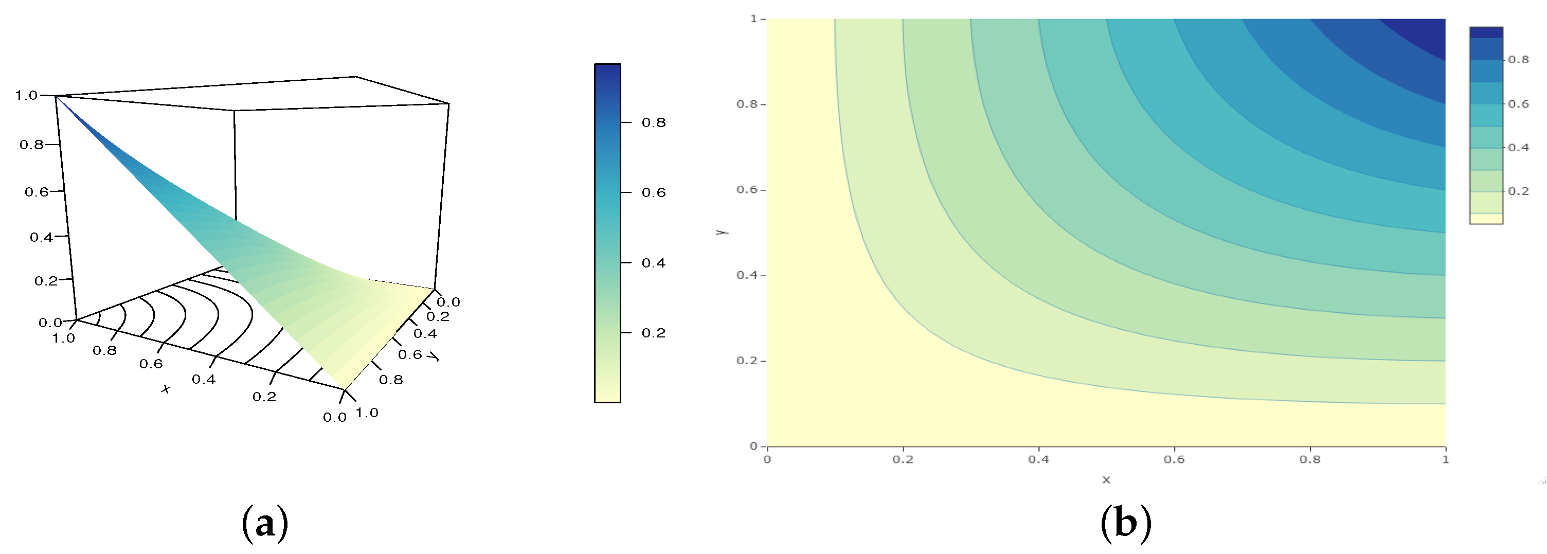
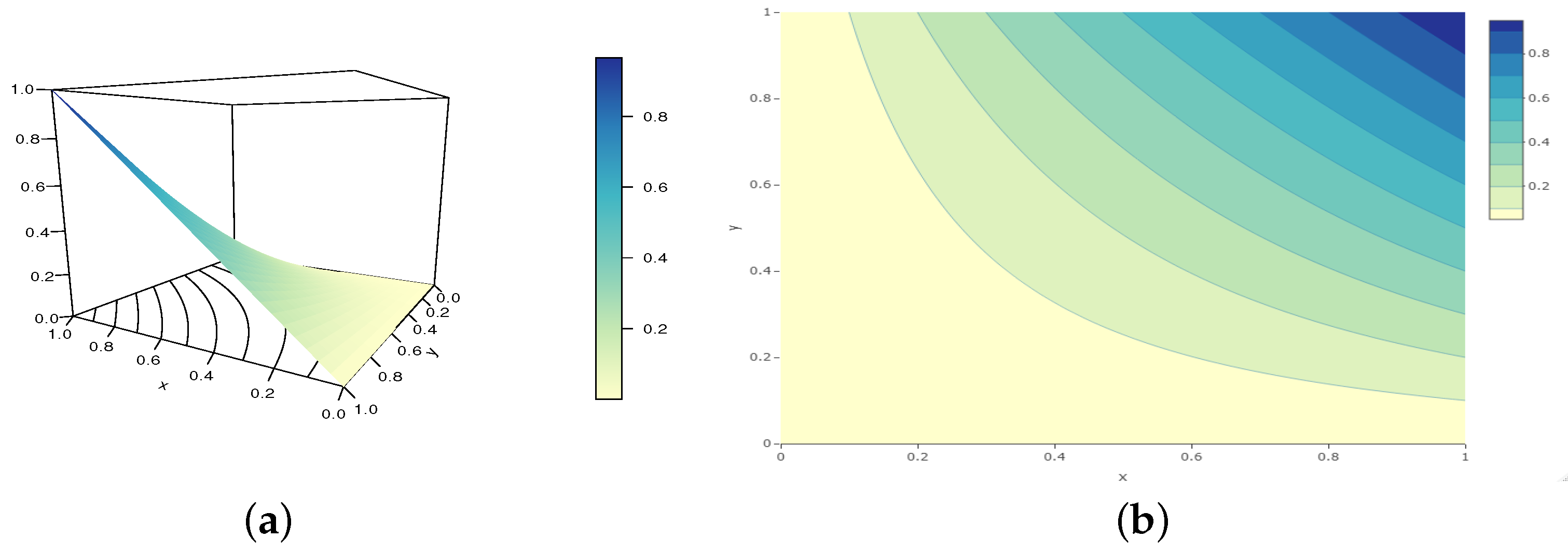
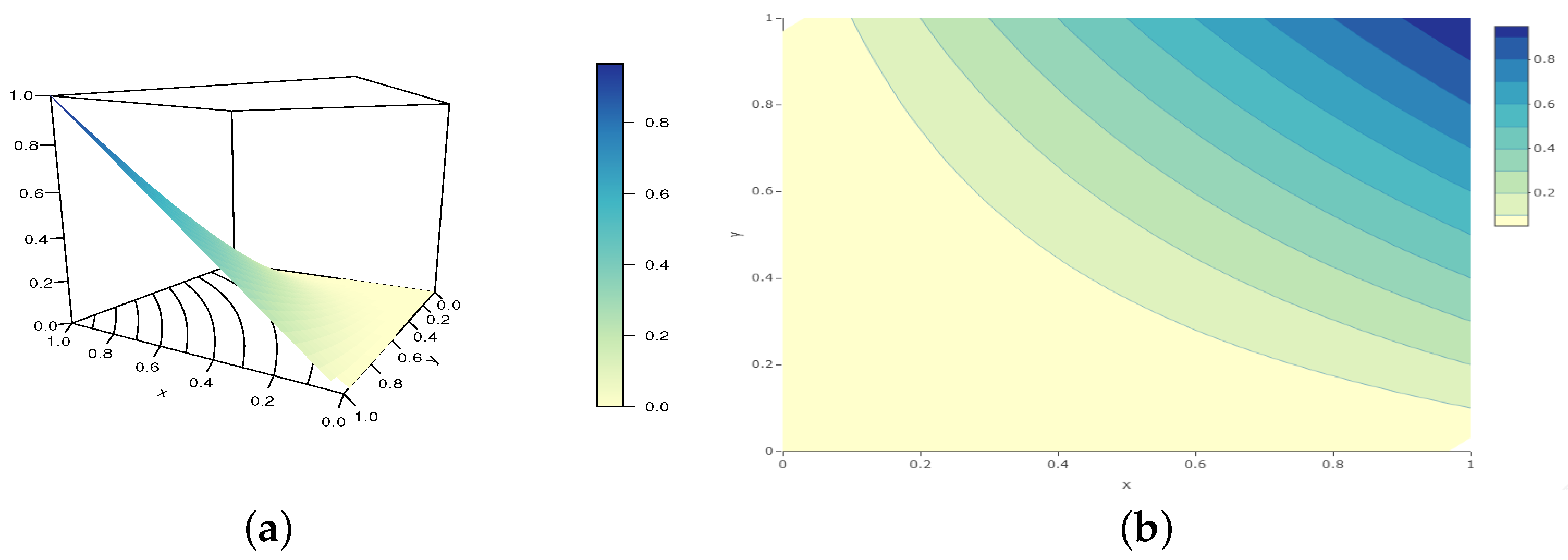
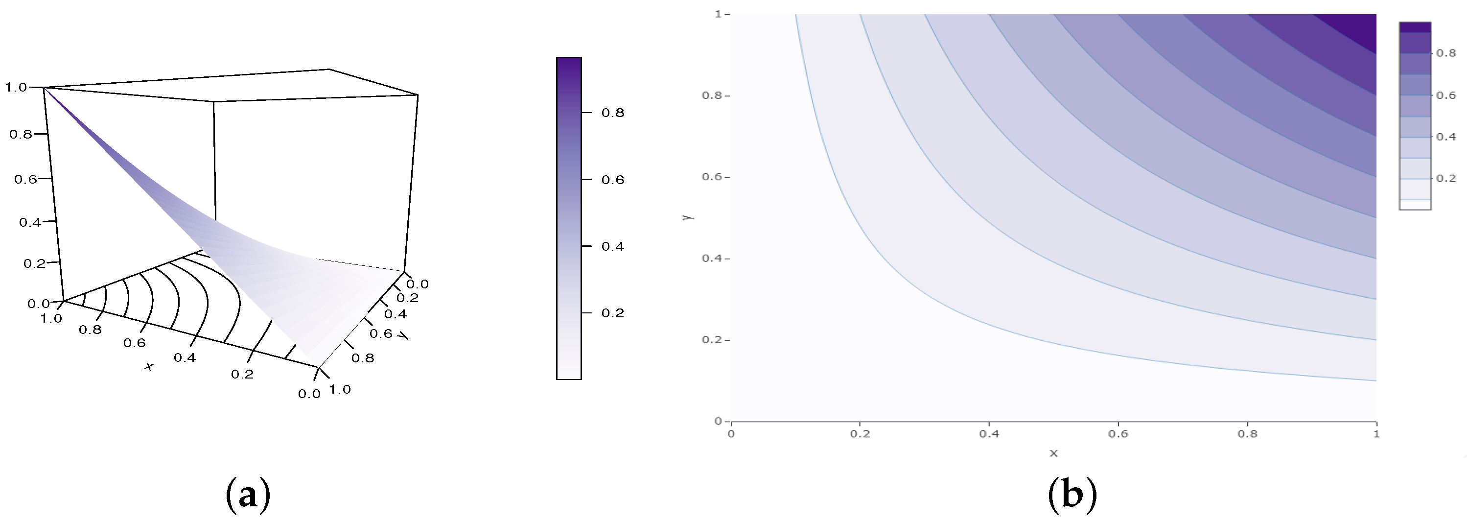
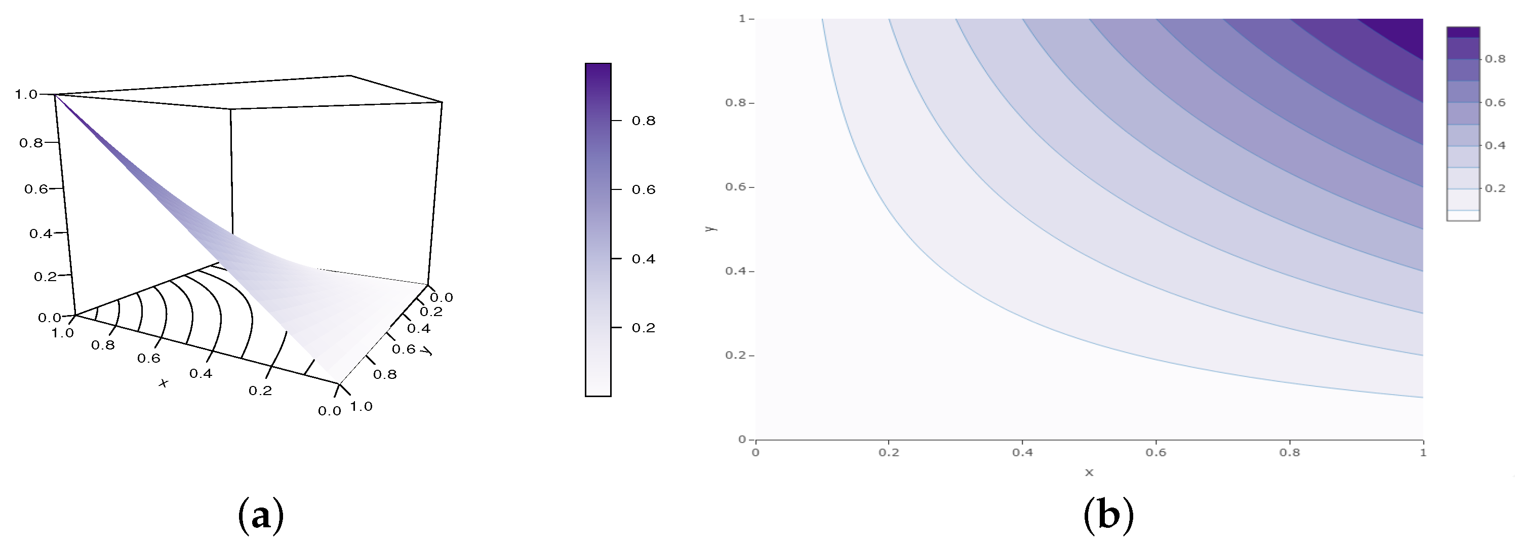
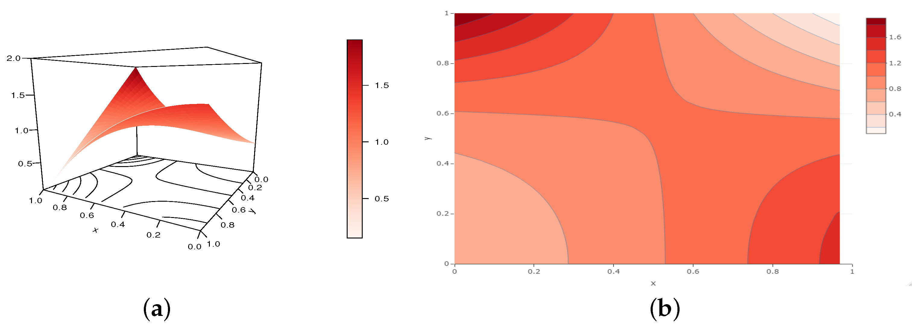
Of course, infinite other examples are possible. Perspective and contour plots of the GCC copula are presented in Figure 1, Figure 2 and Figure 3 for various parameter values belonging to Configurations 1–3, respectively.

Figure 1. Illustrations of the (a) perspective plot and (b) contour plot of the GCC copula for the following configuration: $a=1/2$ and $b=c=2$, belonging to Configuration 1.

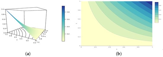
Figure 2. Illustrations of the (a) perspective plot and (b) contour plot of the GCC copula for the following configuration: $a=-1/2$, $b=2$, and $c=1$, belonging to Configuration 2.

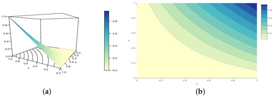
Figure 3. Illustrations of the (a) perspective plot and (b) contour plot of the GCC copula for the following configuration: $a=-2$ and $b=c=-1/2$, belonging to Configuration 3.

From these figures, it is clear that the GCC copula is valid for the considered parameter values. In addition, they demonstrate how the parameters a, b, and c influence the shapes of the GCC copula.

Some important functions related to the GCC copula are presented below.

2.2. Central Functions

Based on the GCC copula, the GCC copula density is the function $c_1(·;\theta ):I\to [0,1]$ indicated as

$$\begin{array}{cc}\hfill c_1(x,y;\theta )& =\frac{{\partial }^2}{\partial x\partial y}{C}_1(x,y;\theta )=exp\left[a(1-x^b)(1-x^c)\right]\times \hfill \\ \hfill & \left[a^{2}bc{x}^b{y}^c(1-x^b)(1-y^c)+(ab+ac+abc)x^b{y}^c-ab{x}^b-ac{y}^c+1\right],(x,y)\in I.\hfill \end{array}$$

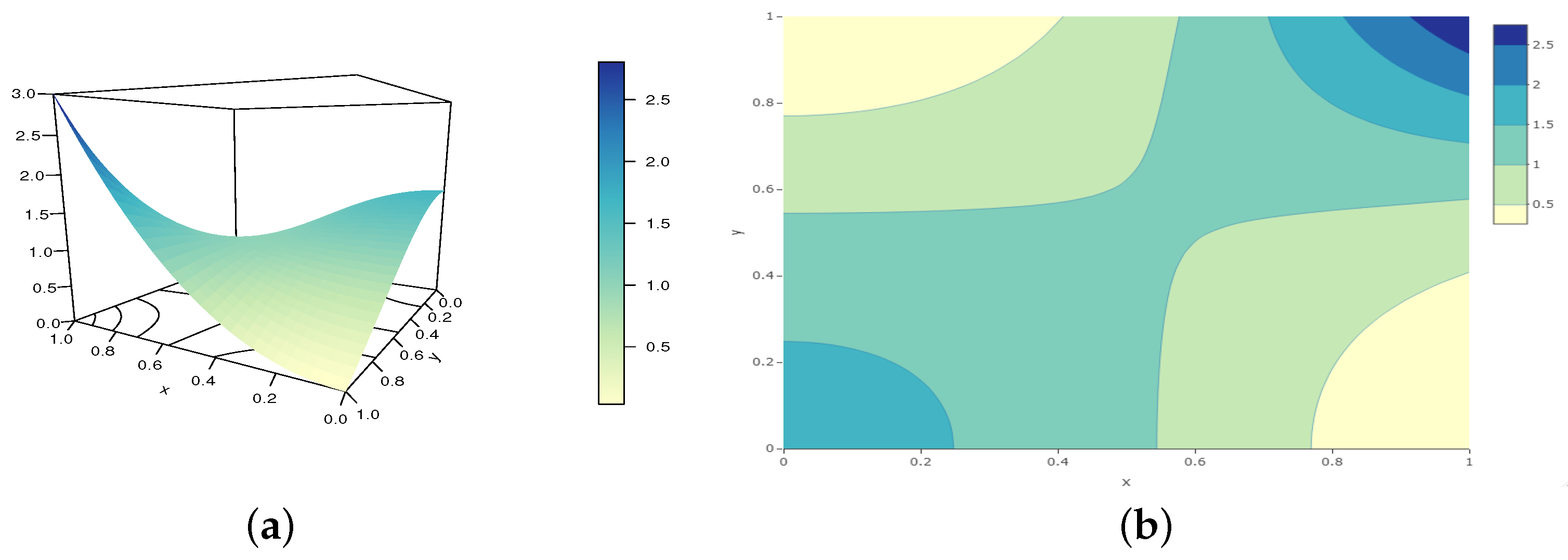
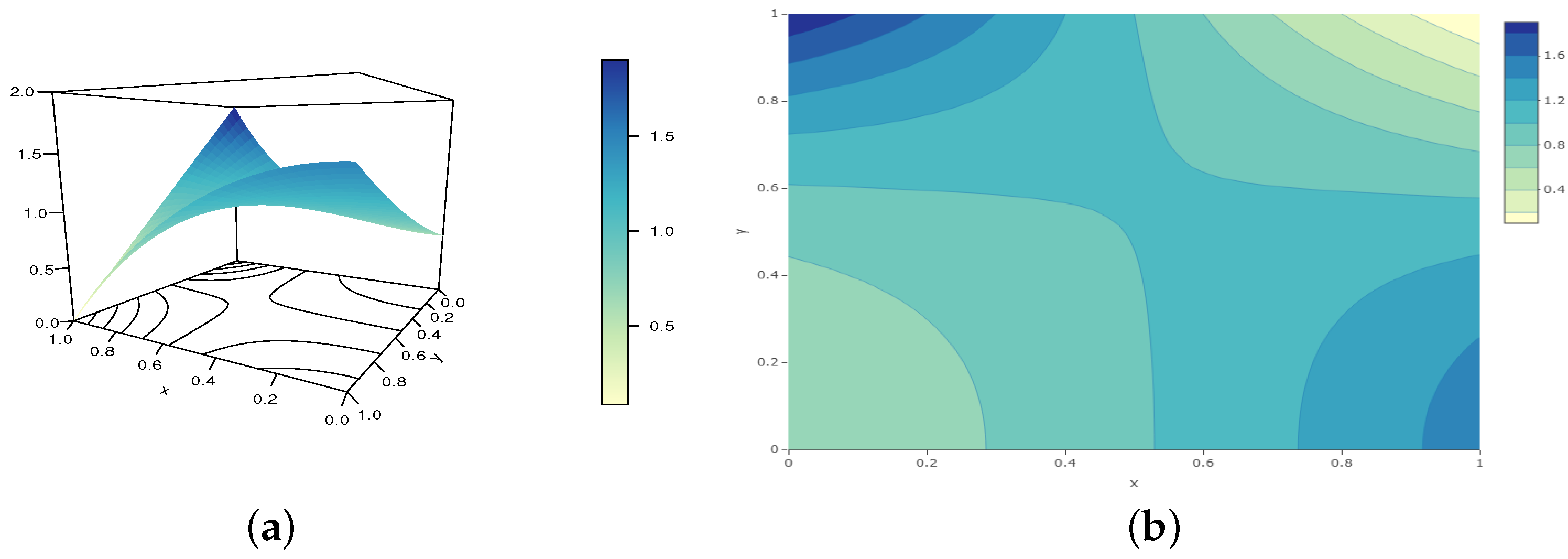
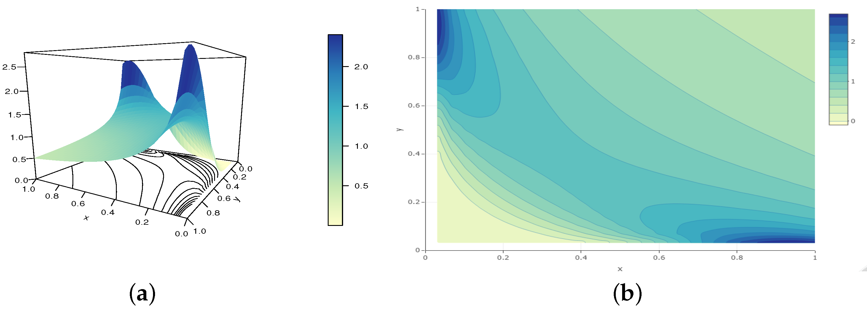
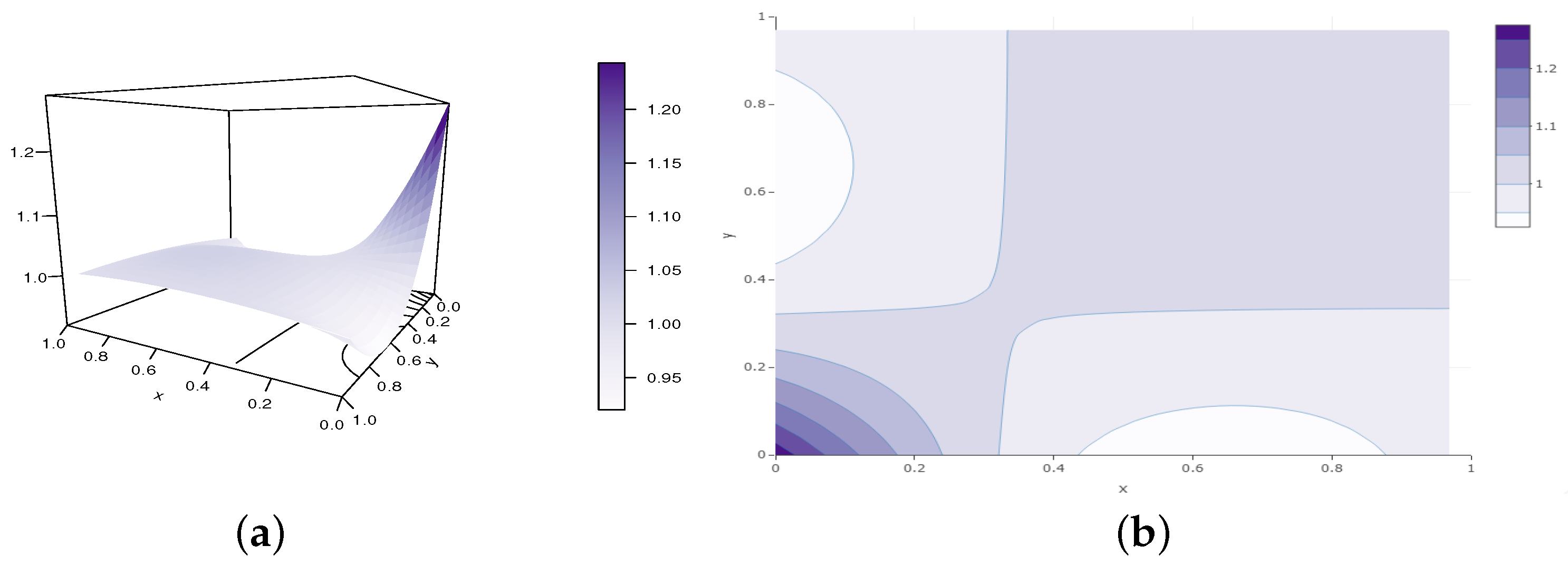
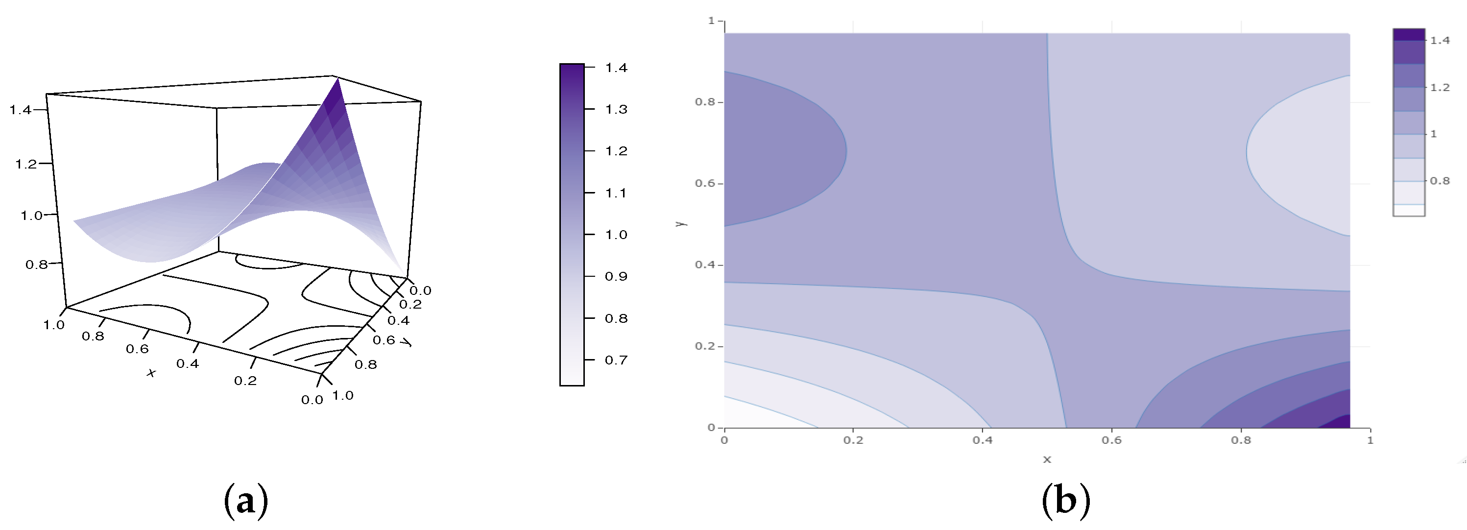
The possible shapes of this function characterize the modeling capability of the GCC copula. With this in mind, Figure 4, Figure 5 and Figure 6 present the perspective and contour plots of this copula density for parameter values belonging to Configurations 1–3, respectively.

Figure 4. Illustrations of the (a) perspective plot and (b) contour plot of the GCC copula density for the following configuration: $a=1/2$ and $b=c=2$, belonging to Configuration 1.

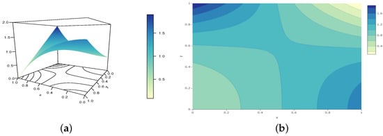
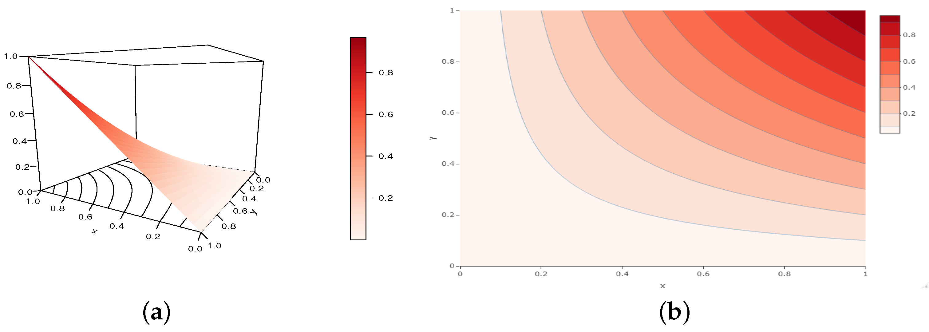
Figure 5. Illustrations of the (a) perspective plot and (b) contour plot of the GCC copula density for the following configuration: $a=-1/2$, $b=2$, and $c=1$, belonging to Configuration 2.

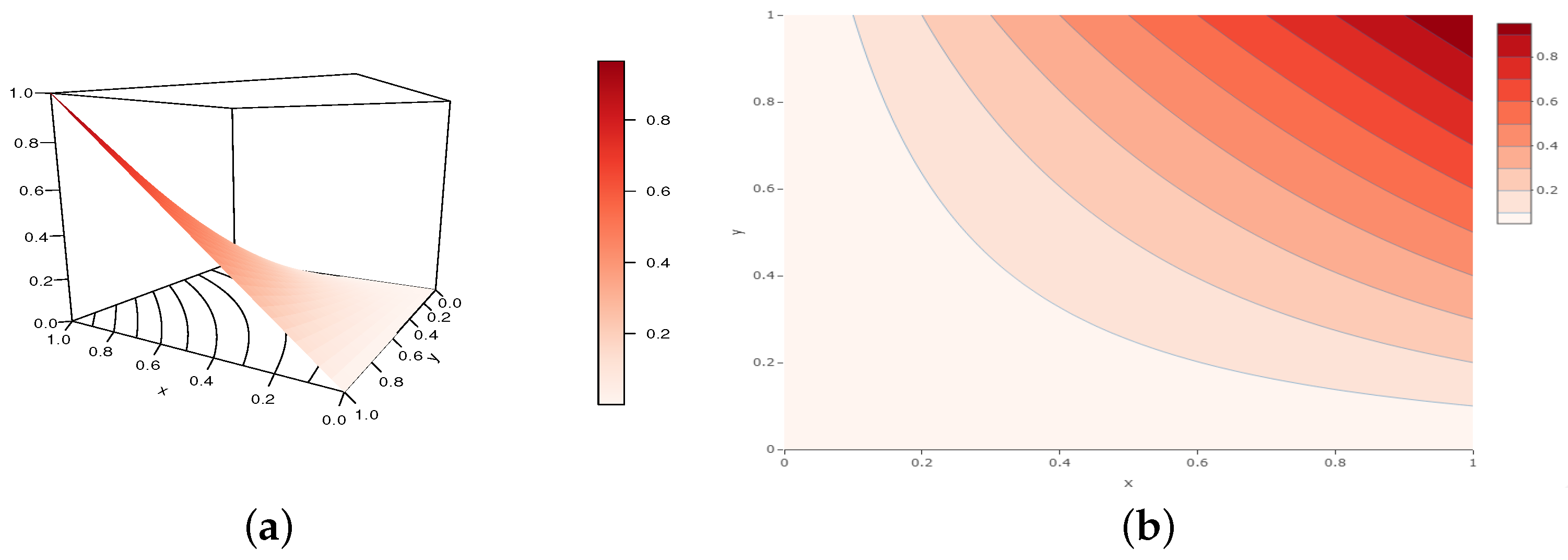
Figure 6. Illustrations of the (a) perspective plot and (b) contour plot of the GCC copula density for the following configuration: $a=-2$ and $b=c=-1/2$, belonging to Configuration 3.

From these figures, we see how the parameters a, b, and c affect the shapes of the GCC copula density; really different shapes are obtained. Figure 6 shows particularly abrupt changes at the extrema that are not observed in Figure 4 and Figure 5. This highlights the singularity of Configuration 3.

The copula density plays a major role in the practical aspect; it is involved in various copula estimation methods, such as the maximum likelihood and the semiparametric estimation. These methods and computationally appealing parametric inference algorithms are treated and reviewed in detail in [24,25]. From a conceptual standpoint, there appears to be no impediment to the simultaneous estimation of the parameters a, b, and c of the GCC copula.

As a last important function, the survival GCC copula is the function ${\widehat{C}}_1(·;\theta ):I\to [0,1]$ defined by

$$\begin{array}{cc}\hfill & {\widehat{C}}_1(x,y;\theta )=x+y-1+C_1(1-x,1-y;\theta )\hfill \\ \hfill & =x+y-1+(1-x)(1-y)exp\left\{a[1-{(1-x)}^b][1-{(1-y)}^c]\right\},(x,y)\in I.\hfill \end{array}$$

It is a valid copula under Configurations 1–3, and it also defines a new copula with the same analytical components as the GCC copula.

2.3. Key Characteristics

Some key characteristics of the GCC copula under Configurations 1–3, are now discussed.

• For $a=0$ or $b=c$, the GCC copula is symmetric since $C_1(x,y;\theta )=C_1(y,x;\theta )$ for any $(x,y)\in I$. For $a\ne 0$ and $b\ne c$, it is not symmetric.
• In full generality, for $a\ne 0$, the GCC copula is not Archimedean, since the CC copula is not. Indeed, for $a=b=c=1$, that is $\theta =(1,1,1)$, we have

  $$\begin{array}{c}\hfill C_1\left(\frac{1}{4},C_1\left(\frac{1}{2},\frac{1}{3};\theta \right);\theta \right)=0.1033978\ne 0.1045974=C_1\left(C_1\left(\frac{1}{4},\frac{1}{2};\theta \right),\frac{1}{3};\theta \right).\end{array}$$

  (3)
  For more detail on this condition, see [4]. Similar numerical results can be proved for other values arbitrarily chosen in Configurations 1–3.
• For $a\ne 0$, the GCC copula is not radially symmetric because there exists $(x,y)$ such that ${\widehat{C}}_1(x,y;\theta )\ne C_1(x,y;\theta )$.
• The GCC copula is positively quadrant dependent for $a\ge 0$ (corresponding to Configuration 1) since $C_1(x,y;\theta )\ge xy$ for any $(x,y)\in I$. It is negatively quadrant dependent for $a<0$ (corresponding to Configurations 2 and 3) since $C_1(x,y;\theta )\le xy$ for any $(x,y)\in I$.
• Using the following inequality: $e^u\ge 1+u$ for any $u\in \mathbb{R}$, for any $(x,y)\in I$, we have

  $$C_1(x,y;\theta )\ge C_{*}(x,y;\theta ),$$

  where $C_{*}(x,y;\theta )=xy\left[1+a(1-x^b)(1-y^c)\right]$. For some values of the parameters, $C_{*}(x,y;\theta )$ represents the first generalized FGM copula described in [23]. Hence, for some parameter values, $C_{*}(x,y;\theta )$ is smaller than $C_1(x,y;\theta )$ with respect to the concordance ordering.
• Using the following inequality: $e^{-u}\ge 1-u$ for any $u\in \mathbb{R}$, for a, b, and c, such that $u=a(1-x^b)(1-y^c)<1$ for any $(x,y)\in I$, we have

  $$C_1(x,y;\theta )\le C_{\diamond }(x,y;\theta ),$$

  where

  $$C_{\diamond }(x,y;\theta )=\frac{xy}{1-a(1-x^b)(1-y^c)}.$$
  For some values of the parameters, $C_{\diamond }(x,y;\theta )$ represents a generalized AMH copula. Hence, for some parameter values, $C_1(x,y;\theta )$ is smaller than $C_{\diamond }(x,y;\theta )$ with respect to the concordance ordering.
• The Fréchet–Hoeffding (FH) bounds are satisfied, as for any copula. More precisely, for any $(x,y)\in I$, we have $max(x+y-1,0)\le C_1(x,y;\theta )\le min(x,y)$.
• Using the exponential series and binomial expansions, the GCC copula can be expressed as

  $$\begin{array}{c}\hfill C_1(x,y;\theta )=\sum _{i=0}^{\infty }\sum _{j=0}^i\sum _{k=0}^i{\alpha }_{i,j,k}{x}^{bj+1}{y}^{ck+1},\end{array}$$

  (4)

  where

  $${\alpha }_{i,j,k}=\frac{a^i}{i!}\left(\genfrac{}{}{0pt}{}{i}{j}\right)\left(\genfrac{}{}{0pt}{}{i}{k}\right){(-1)}^{j+k}.$$
  The binomial coefficient is standardly defined as $\left(\genfrac{}{}{0pt}{}{z}{k}\right)=z(z-1)(z-2)\dots (z-k+1)/(k!)$. Similarly, the GCC copula density can be expanded as

  $$c_1(x,y;\theta )=\sum _{i=0}^{\infty }\sum _{j=0}^i\sum _{k=0}^i{\beta }_{i,j,k}{x}^{bj}{y}^{ck},$$

  where ${\beta }_{i,j,k}=(bj+1)(ck+1){\alpha }_{i,j,k}$. Approximations for various moment analyses are possible as a result of this expansion.
• Using classical limit techniques, we obtain

  $${\lambda }_L=\underset{x\to 0}{lim}\frac{C_1(x,x;\theta )}{x}=\underset{x\to 0}{lim}xexp\left[a(1-x^b)(1-x^c)\right]=0$$

  and

  $${\lambda }_U=\underset{x\to 1}{lim}\frac{1-2x+C_1(x,x;\theta )}{1-x}=\underset{x\to 1}{lim}\frac{1-2x+x^{2}exp\left[a(1-x^b)(1-x^c)\right]}{1-x}=0.$$
  Hence, there is no tail dependence in the GCC copula.
• The medial correlation (or Blomqvist coefficient) of the GCC copula is indicated as

  $$M=4C_1\left(\frac{1}{2},\frac{1}{2};\theta \right)-1=exp\left[a(1-2^{-b})(1-2^{-c})\right]-1.$$
  Table 1, Table 2 and Table 3 present the numerical values (rounded to the second decimal) for $\theta =(\gamma ,1/\gamma ,1/\gamma )$, $\theta =(-1/\gamma ,\sqrt{\gamma },\sqrt{\gamma })$, and $\theta =(-1/\gamma ,-\gamma ,-1)$, for several positive values of $\gamma$, being special examples of Configurations 1–3, respectively. In fact, for the values of gamma in the tables that follow, the grid $0.01$, $0.09$, $0.17$, $0.25$, $0.33$, $0.41$, $0.49$, $0.57$, $0.65$, $0.73$, $0.81$, $0.89$ is arbitrarily chosen, making all the future proposed copulas mathematically valid.
  Table 1. Values of the medial correlation of the GCC copula for $\theta =(\gamma ,1/\gamma ,1/\gamma )$ and several values of $\gamma$, belonging to Configuration 1.

  $\gamma$	0.01	0.09	0.17	0.25	0.33	0.41	0.49	0.57	0.65	0.73	0.81	0.89
  M	0.01	0.09	0.18	0.25	0.29	0.31	0.32	0.33	0.32	0.32	0.31	0.3

  Table 2. Values of the medial correlation of the GCC copula for $\theta =(-1/\gamma ,\sqrt{\gamma },\sqrt{\gamma })$ and several values of $\gamma$, belonging to Configuration 2.

  $\gamma$	0.01	0.09	0.17	0.25	0.33	0.41	0.49	0.57	0.65	0.73	0.81	0.89
  M	−0.36	−0.32	−0.3	−0.29	−0.28	−0.27	−0.26	−0.25	−0.25	−0.24	−0.23	−0.23

  Table 3. Values of the medial correlation of the GCC copula for $\theta =(-1/\gamma ,-\gamma ,-1)$ and several values of $\gamma$, belonging to Configuration 3.

  $\gamma$	0.01	0.09	0.17	0.25	0.33	0.41	0.49	0.57	0.65	0.73	0.81	0.89
  M	−0.5	−0.51	−0.52	−0.53	−0.54	−0.55	−0.56	−0.57	−0.58	−0.59	−0.61	−0.62

  From these tables, it can be seen that a negative or positive medial correlation can be reached with a moderate wide amplitude of values (here, for the considered parameter values, from $-0.62$ to $0.3$).
• The rho of Spearman of the GCC copula is defined by

  $$\rho =12{\int }_0^1{\int }_0^1\left[C_1(x,y;\theta )-xy\right]dxdy.$$
  No closed-form expression exists. However, by using Equation (4), we can express it as

  $$\rho =12\sum _{i=1}^{\infty }\sum _{j=0}^i\sum _{k=0}^i{\alpha }_{i,j,k}\frac{1}{(bj+2)(ck+2)}.$$
  Table 4, Table 5 and Table 6 present its numerical values (rounded to the second decimal) for $\theta =(\gamma ,1/\gamma ,1/\gamma )$, $\theta =(-1/\gamma ,\sqrt{\gamma },\sqrt{\gamma })$, and $\theta =(-1/\gamma ,-\gamma ,-1)$, for several positive values of $\gamma$, being special examples of Configurations 1–3, respectively.
  Table 4. Values of the rho of Spearman of the GCC copula for $\theta =(\gamma ,1/\gamma ,1/\gamma )$ and several values of $\gamma$, belonging to Configuration 1.

  $\gamma$	0.01	0.09	0.17	0.25	0.33	0.41	0.49	0.57	0.65	0.73	0.81	0.89
  $\rho$	0.03	0.2	0.3	0.36	0.4	0.41	0.42	0.42	0.42	0.41	0.4	0.39

  Table 5. Values of the rho of Spearman of the GCC copula for $\theta =(-1/\gamma ,\sqrt{\gamma },\sqrt{\gamma })$ and several values of $\gamma$, belonging to Configuration 2.

  $\gamma$	0.01	0.09	0.17	0.25	0.33	0.41	0.49	0.57	0.65	0.73	0.81	0.89
  $\rho$	−0.5	−0.44	−0.41	−0.39	−0.38	−0.36	−0.35	−0.34	−0.33	−0.32	−0.31	−0.31

  Table 6. Values of the rho of Spearman of the GCC copula for $\theta =(-1/\gamma ,-\gamma ,-1)$ and several values of $\gamma$, belonging to Configuration 3.

  $\gamma$	0.01	0.09	0.17	0.25	0.33	0.41	0.49	0.57	0.65	0.73	0.81	0.89
  $\rho$	−0.68	−0.69	−0.71	−0.72	−0.73	−0.74	−0.75	−0.77	−0.78	−0.79	−0.8	−0.82

  These tables demonstrate that the rho of Spearman of the GCC copula can be either negative or positive with wide amplitude (here, from $-0.82$ to $0.39$). It can be non-monotonic according to the parameters. Thus, the GCC copula is ideal for modeling various kinds of dependence.
• Let $F\left(x\right)$ and $G\left(x\right)$ be two unidimensional CDFs. Then, under Configurations 1–3, we define a new two-dimensional CDF by considering the function $H:I\to [0,1]$ indicated as $H(x,y;\theta )=C_1(F\left(x\right),G\left(y\right);\theta )$. Thus, based on this function, there are an endless number of potential new two-dimensional distributions. For choices of motivated lifetime CDFs for $F\left(x\right)$ and $G\left(x\right)$, we refer to [26].

The section below explores another possible generalized GCC copula, following the second generalization scheme of [23].

3. Second Generalized CC Copula

3.1. Presentation and Result

The second proposed generalized CC copula is indicated in the proposition below.

Proposition 2.

Let $\theta =(a,b,c)\in {\mathbb{R}}^3$. We consider the function $C_2(·;\theta ):I\to [0,1]$ defined by

$$\begin{array}{c}\hfill C_2(x,y;\theta )=xyexp\left[a{(1-x)}^b{(1-y)}^c\right],(x,y)\in I.\end{array}$$

(5)

Then, $C_2(x,y;\theta )$ is a copula for the following parameter configurations (non-overlapping):

Configuration 1:

$a\ge 0$, $b\ge 1$, $c\ge 1$, $ab\le 1$, and $ac\le 1$.

Configuration 2:

$a<0$, $b\ge 1$, $c\ge 1$, and $abc\ge -1$.

Proof. 

As for the proof of Proposition 1, the proof is based on Definition 1 using differentiation, well-chosen factorization techniques, and inequalities. The two different parameter configurations will be conjointly assumed for (i) and (ii), but they will be distinguished for (iii).

(i) 

For any $x\in [0,1]$, we have $C_2(x,0;\theta )=x\times 0\times exp\left[a{(1-x)}^b{(1-0)}^c\right]=0$, and, similarly, for any $y\in [0,1]$, $C_2(0,y;\theta )=0$.

(ii) 

For any $x\in [0,1]$, we have $C_2(x,1;\theta )=x\times 1\times exp\left[a{(1-x)}^b{(1-1)}^c\right]=x$, and, similarly, for any $y\in [0,1]$, $C_2(1,y;\theta )=y$.

(iii) 

For any $(x,y)\in I$, using standard differentiation techniques and well-chosen factorizations, we obtain

$$\begin{array}{cc}\hfill & \frac{{\partial }^2}{\partial x\partial y}{C}_2(x,y;\theta )={(1-x)}^{-1}{(1-y)}^{-1}exp\left[a{(1-x)}^b{(1-y)}^c\right]\times \hfill \\ \hfill & \left[a^{2}bcxy{(1-x)}^{2b}{(1-y)}^{2c}+{(1-x)}^b{(1-y)}^c[(ab+ac+abc)xy-abx-acy]+(1-x)(1-y)\right]\hfill \\ \hfill & ={(1-x)}^{-1}{(1-y)}^{-1}exp\left[a{(1-x)}^b{(1-y)}^c\right]\times \hfill \\ \hfill & \left[f(x,y;\theta )+{(1-x)}^b{(1-y)}^{c}g(x,y;\theta )+h(x,y;\theta )\right],\hfill \end{array}$$

where

$$f(x,y;\theta )=a^{2}bcxy{(1-x)}^{2b}{(1-y)}^{2c},g(x,y;\theta )=(ab+ac+abc)xy-abx-acy+1$$

and

$$h(x,y;\theta )=(1-x)(1-y)-{(1-x)}^b{(1-y)}^c.$$

Let us demonstrate that these functions are positive under the two different parameter configurations.

Configuration 1:

We recall that $a\ge 0$, $b\ge 1$, $c\ge 1$, $ab\le 1$, and $ac\le 1$. For any $(x,y)\in I$, since $a\ge 0$, $b\ge 1$, and $c\ge 1$, it is clear that $f(x,y;\theta )\ge 0$ and $h(x,y;\theta )\ge 0$. Now, we can decompose $g(x,y;\theta )$ as

$$g(x,y;\theta )=(1-abx)(1-acy)+a(b+(1-ab)c+bc)xy.$$

For $a\ge 0$, $b\ge 1$, $c\ge 1$, $ab\le 1$, and $ac\le 1$, we get $g(x,y;\theta )\ge 0$ as a sum of positive functions. Hence

$$\frac{{\partial }^2}{\partial x\partial y}{C}_2(x,y;\theta )\ge 0.$$

Configuration 2:

We recall that $a<0$, $b\ge 1$, $c\ge 1$, and $abc\ge -1$. For any $(x,y)\in I$, since $a<0$, $b\ge 1$, and $c\ge 1$, it is clear that $f(x,y;\theta )\ge 0$ and $h(x,y;\theta )\ge 0$. Now, we can express $g(x,y;\theta )$ as

$$g(x,y;\theta )=-ac(1-x)y+1+abx\left[\right(c+1)y-1].$$

For $a<0$, $b\ge 1$, and $c\ge 1$, we have $-ac(1-x)y\ge 0$ and $a\left[\right(c+1)y-1]\ge ac$, and it follows from $abc\ge -1$ that

$$g(x,y;\theta )\ge 1+abcx\ge 1+abc\ge 0.$$

Hence

$$\frac{{\partial }^2}{\partial x\partial y}{C}_2(x,y;\theta )\ge 0.$$

Thus, the point (iii) is demonstrated for the two configurations.

The full proof of Proposition 2 ends. □

For the purposes of this study, the copula presented in Equation (5) is called the second generalized CC (SGCC) copula. It is worth noting that in Configurations 1 and 2 of Proposition 2, we have $b\ge 1$ and $c\ge 1$, which seem crucial to have a valid copula. As for the GCC copula, the CC copula is obtained by taking $a\in [-1,1]$ and $b=c=1$, which are parameter values that combine those in the two configurations. To the best of our knowledge, the SGCC copula and these clear parameter configurations are new in the literature. Based on Proposition 2, some parameter configuration examples with only one tuning parameter are given below.

Example 1:

For any $\gamma \in (0,1]$, Configuration 1 includes $a=\gamma$ and $b=c=1/\gamma$, that is

$$\theta =\left(\gamma ,\frac{1}{\gamma },\frac{1}{\gamma }\right).$$

Example 2:

For any $\gamma \in (0,1]$, Configuration 2 includes $a=-\gamma$, and $b=c=1/\sqrt{\gamma }$, that is

$$\theta =\left(-\gamma ,\frac{1}{\sqrt{\gamma }},\frac{1}{\sqrt{\gamma }}\right).$$

These are just a few examples of the infinite number of possible combinations. Perspective and contour plots of the SGCC copula are presented in Figure 7 and Figure 8 for parameter values belonging to Configurations 1 and 2, respectively.

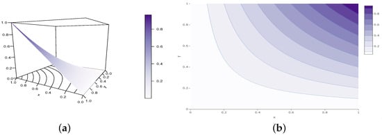
Figure 7. Illustrations of the (a) perspective plot and (b) contour plot of the SGCC copula for the following configuration: $a=1/4$ and $b=c=2$, belonging to Configuration 1.

Figure 8. Illustrations of the (a) perspective plot and (b) contour plot of the SGCC copula for the following configuration: $a=-1/2$, $b=2$, and $c=1$, belonging to Configuration 2.

These figures make it obvious that the SGCC copula holds true for the parameter values under consideration. Furthermore, they show how the shapes of the SGCC copula are affected by the parameters a, b, and c.

Some important functions related to the SGCC copula are presented below.

3.2. Central Functions

Based on the SGCC copula, the SGCC copula density is the function $c_2(·;\theta ):I\to [0,1]$ indicated as

$$\begin{array}{cc}\hfill & c_2(x,y;\theta )=\frac{{\partial }^2}{\partial x\partial y}{C}_2(x,y;\theta )\hfill \\ \hfill & ={(1-x)}^{-1}{(1-y)}^{-1}exp\left[a{(1-x)}^b{(1-y)}^c\right]\times \hfill \\ \hfill & \left[a^{2}bcxy{(1-x)}^{2b}{(1-y)}^{2c}+{(1-x)}^b{(1-y)}^c[(ab+ac+abc)xy-abx-acy]+(1-x)(1-y)\right],\hfill \\ \hfill & (x,y)\in I.\hfill \end{array}$$

The possible shapes of this function characterize the modeling capability of the SGCC copula. As a visual approach, the perspective and contour plots of this copula density for parameter values belonging to Configurations 1 and 2 are shown in Figure 9 and Figure 10, respectively.

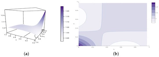
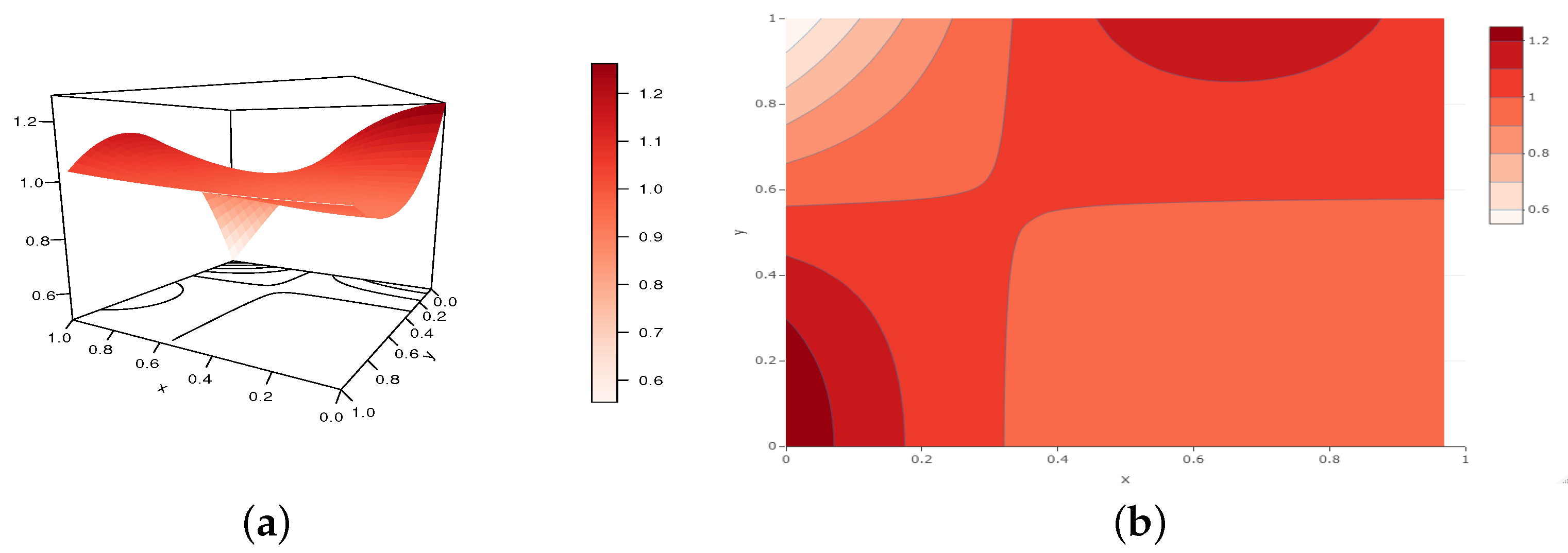
Figure 9. Illustrations of the (a) perspective plot and (b) contour plot of the SGCC copula density for the following configuration: $a=1/4$ and $b=c=2$, belonging to Configuration 1.

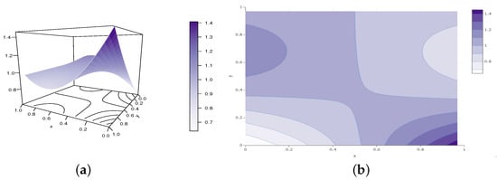
Figure 10. Illustrations of the (a) perspective plot and (b) contour plot of the SGCC copula density for the following configuration: $a=-1/2$, $b=2$, and $c=1$, belonging to Configuration 2.

From these figures, we see how the parameters a, b, and c affect the shapes of the SGCC copula density.

As a last important function, the survival SGCC copula is the function ${\widehat{C}}_2(·;\theta ):I\to [0,1]$ defined by

$$\begin{array}{cc}\hfill & {\widehat{C}}_2(x,y;\theta )=x+y-1+C_2(1-x,1-y;\theta )\hfill \\ \hfill & =x+y-1+(1-x)(1-y)exp\left(a{x}^b{y}^c\right),(x,y)\in I.\hfill \end{array}$$

Under Configurations 1 and 2, it defines a legitimate copula and has the same analytical elements as the SGCC copula.

3.3. Key Characteristics

Some key characteristics of the SGCC copula under Configurations 1 and 2 are now discussed.

• For $a=0$ or $b=c$, the SGCC copula is symmetric, since $C_2(x,y;\theta )=C_2(y,x;\theta )$ for any $(x,y)\in I$. For $a\ne 0$, and $b\ne c$, it is not symmetric.
• For $a\ne 0$, the SGCC copula is not Archimedean. For instance, for $a=b=1$, that is $\theta =(1,1,1)$, Equation (3) still holds since, in this case, $C_2(x,y;\theta )=C_1(x,y;\theta )$.
• For $a\ne 0$, the SGCC copula is not radially symmetric because there exists $(x,y)$ such that ${\widehat{C}}_2(x,y;\theta )\ne C_2(x,y;\theta )$.
• The SGCC copula is positively quadrant dependent for $a\ge 0$ (corresponding to Configuration 1), since $C_2(x,y;\theta )\ge xy$ for any $(x,y)\in I$. It is negatively quadrant dependent for $a<0$ (corresponding to Configuration 2) since $C_2(x,y;\theta )\le xy$ for any $(x,y)\in I$.
• Using the following inequality: $e^u\ge 1+u$ for any $u\in \mathbb{R}$, for any $(x,y)\in I$, we obtain

  $$C_2(x,y;\theta )\ge C_{\circ }(x,y;\theta ),$$

  where $C_{\circ }(x,y;\theta )=xy\left[1+a{(1-x)}^b{(1-y)}^c\right]$. For some values of the parameters, $C_{\circ }(x,y;\theta )$ represents the second generalized FGM copula described in [23]. Hence, for some parameter values, $C_{\circ }(x,y;\theta )$ is smaller than $C_2(x,y;\theta )$ with respect to the concordance ordering.
• Using the following inequality: $e^{-u}\ge 1-u$ for any $u\in \mathbb{R}$, for a, b, and c, such that $u=a{(1-x)}^b{(1-y)}^c<1$ for any $(x,y)\in I$, we have

  $$C_2(x,y;\theta )\le C_{▹}(x,y;\theta ),$$

  where

  $$C_{▹}(x,y;\theta )=\frac{xy}{1-a{(1-x)}^b{(1-y)}^c}.$$
  For some values of the parameters, $C_{▹}(x,y;\theta )$ represents a generalized AMH copula. Hence, for some parameter values, $C_2(x,y;\theta )$ is smaller than $C_{▹}(x,y;\theta )$ with respect to the concordance ordering.
• In full generality, there is no immediate concordance ordering between the GCC and SGCC copulas.
• The FH bounds hold.
• For $(x,y)\in {[0,1)}^2$, using the exponential series and generalized binomial expansions, the SGCC copula can be expressed as

  $$\begin{array}{c}\hfill C_2(x,y;\theta )=\sum _{i=0}^{\infty }\sum _{j=0}^{\infty }\sum _{k=0}^{\infty }{\mu }_{i,j,k}{x}^{j+1}{y}^{k+1},\end{array}$$

  (6)

  where

  $${\mu }_{i,j,k}=\frac{a^i}{i!}\left(\genfrac{}{}{0pt}{}{bi}{j}\right)\left(\genfrac{}{}{0pt}{}{ci}{k}\right){(-1)}^{j+k}.$$
  Similarly, the SGCC copula density can be expanded as

  $$c_2(x,y;\theta )=\sum _{i=0}^{\infty }\sum _{j=0}^i\sum _{k=0}^i{\nu }_{i,j,k}{x}^j{y}^k,$$

  where ${\nu }_{i,j,k}=(j+1)(k+1){\mu }_{i,j,k}$. Approximations for various moment analyses are possible as a result of this expansion.
• Let us now investigate the possible tail dependence of the SGCC copula. Using standard limit techniques, we have

  $${\lambda }_L=\underset{x\to 0}{lim}\frac{C_2(x,x;\theta )}{x}=\underset{x\to 0}{lim}xexp\left[a{(1-x)}^{b+c}\right]=0$$

  and

  $${\lambda }_U=\underset{x\to 1}{lim}\frac{1-2x+C_2(x,x;\theta )}{1-x}=\underset{x\to 1}{lim}\frac{1-2x+x^{2}exp\left[a{(1-x)}^{b+c}\right]}{1-x}=0.$$
  As a result, the SGCC copula has no tail dependence.
• The medial correlation of the SGCC copula is simply indicated as

  $$M=4C_2\left(\frac{1}{2},\frac{1}{2};\theta \right)-1=exp\left(a{2}^{-(b+c)}\right)-1.$$
  As numerical works, Table 7 and Table 8 show some numerical values of M for $\theta =(\gamma ,1/\gamma ,1/\gamma )$ and $\theta =(-\gamma ,1/\sqrt{\gamma },1/\sqrt{\gamma })$ (rounded to the second decimal), for several values of $\gamma \in (0,1]$, being special examples of Configurations 1 and 2, respectively.
  Table 7. Values of the medial correlation of the SGCC copula for $\theta =(\gamma ,1/\gamma ,1/\gamma )$ and several values of $\gamma$, belonging to Configuration 1.

  $\gamma$	0.01	0.09	0.17	0.25	0.33	0.41	0.49	0.57	0.65	0.73	0.81	0.89
  M	0	0	0	0	0	0.01	0.03	0.05	0.08	0.12	0.16	0.21

  Table 8. Values of the medial correlation of the SGCC copula for $\theta =(-\gamma ,1/\sqrt{\gamma },1/\sqrt{\gamma })$ and several values of $\gamma$, belonging to Configuration 2.

  $\gamma$	0.01	0.09	0.17	0.25	0.33	0.41	0.49	0.57	0.65	0.73	0.81	0.89
  M	0	0	−0.01	−0.02	−0.03	−0.05	−0.07	−0.09	−0.11	−0.13	−0.16	−0.19

  These tables show that a moderate amplitude of values can result in a medial correlation that is either negative or positive (here, from $-0.19$ to $0.21$).
• The rho of Spearman of the SGCC copula is defined by

  $$\rho =12{\int }_0^1{\int }_0^1\left[C_2(x,y;\theta )-xy\right]dxdy.$$
  Clearly, it does not have a closed-form expression. However, by using Equation (6), we can expand it as

  $$\rho =12\sum _{i=1}^{\infty }\sum _{j=0}^{\infty }\sum _{k=0}^{\infty }{\mu }_{i,j,k}\frac{1}{(j+2)(k+2)}.$$
  Table 9 and Table 10 determine its numerical values for $\theta =(\gamma ,1/\gamma ,1/\gamma )$ and $\theta =(-\gamma ,1/\sqrt{\gamma },1/\sqrt{\gamma })$ (rounded to the second decimal), for several values of $\gamma \in (0,1]$, being special examples of Configurations 1 and 2, respectively.
  Table 9. Values of the rho of Spearman of the SGCC copula for $\theta =(\gamma ,1/\gamma ,1/\gamma )$ and several values of $\gamma$, belonging to Configuration 1.

  $\gamma$	0.01	0.09	0.17	0.25	0.33	0.41	0.49	0.57	0.65	0.73	0.81	0.89
  $\rho$	0	0	0	0	0.01	0.02	0.04	0.07	0.1	0.15	0.2	0.27

  Table 10. Values of the rho of Spearman of the SGCC copula for $\theta =(-\gamma ,1/\sqrt{\gamma },1/\sqrt{\gamma })$ and several values of $\gamma \in (0,1]$, belonging to Configuration 2.

  $\gamma$	0.01	0.09	0.17	0.25	0.33	0.41	0.49	0.57	0.65	0.73	0.81	0.89
  $\rho$	0	0	−0.01	−0.02	−0.04	−0.06	−0.08	−0.11	−0.14	−0.17	−0.21	−0.24

  These tables demonstrate that the rho of Spearman of the SGCC copula can be either negative or positive with wide amplitude (here, from $-0.24$ to $0.27$). Thus, the SGCC copula is ideal to model various kinds of dependence.
• Let $F\left(x\right)$ and $G\left(x\right)$ be two unidimensional CDFs. Then, under Configurations 1 and 2, we define a new two-dimensional CDF by considering the function $H:I\to [0,1]$ indicated as $H(x,y;\theta )=C_2(F\left(x\right),G\left(y\right);\theta )$. Thus, based on this function, there are an endless number of potential new two-dimensional distributions. We again refer to [26] while discussing the options for motivated lifetime CDFs for $F\left(x\right)$ and $G\left(x\right)$.

A third generalized CC copula that mixes the power schemes of the GCC and SGCC copulas is described in the next section.

4. Third Generalized CC Copula

4.1. Presentation and Result

The third proposed generalized CC copula is indicated in the proposition below.

Proposition 3.

Let $\theta =(a,b,c)\in {\mathbb{R}}^3$. We consider the function $C_3(·;\theta ):I\to [0,1]$ defined by

$$\begin{array}{c}\hfill C_3(x,y;\theta )=xyexp\left[a(1-x^b){(1-y)}^c\right],(x,y)\in I.\end{array}$$

(7)

Then, $C_3(x,y;\theta )$ is a copula for the following parameter configurations (non-overlapping):

Configuration 1:

$a\ge 0$, $b>0$, $c\ge 1$, $ab\le 1$, and $ac\le 1$.

Configuration 2:

$a<0$, $b>0$, $c\ge 1$, and $abc\ge -1$.

Proof. 

As for the proof of Propositions 1 and 2, the proof is based on Definition 1 using differentiation, well-chosen factorization techniques, and inequalities. The two different parameter configurations will be conjointly assumed for (i) and (ii), but they will be distinguished for (iii).

(i) 

For any $x\in [0,1]$, we have $C_3(x,0;\theta )=x\times 0\times exp\left[a(1-x^b){(1-0)}^c\right]=0$, and, similarly, for any $y\in [0,1]$, $C_3(0,y;\theta )=0$.

(ii) 

For any $x\in [0,1]$, we have $C_3(x,1;\theta )=x\times 1\times exp\left[a(1-x^b){(1-1)}^c\right]=x$, and, similarly, for any $y\in [0,1]$, $C_3(1,y;\theta )=y$.

(iii) 

Using conventional differentiation methods and carefully chosen factorizations, we obtain, for any $(x,y)\in I$,

$$\begin{array}{cc}\hfill & \frac{{\partial }^2}{\partial x\partial y}{C}_3(x,y;\theta )={(1-y)}^{-1}exp\left[a(1-x^b){(1-y)}^c\right]\times \hfill \\ \hfill & \left[a^{2}bc{x}^{b}y(1-x^b){(1-y)}^{2c}+{(1-y)}^c[(ab+ac+abc)x^{b}y-ab{x}^b-acy]+1-y\right]\hfill \\ \hfill & ={(1-y)}^{-1}exp\left[a(1-x^b){(1-y)}^c\right]\times \hfill \\ \hfill & \left[f(x,y;\theta )+{(1-y)}^{c}g(x,y;\theta )+h(x,y;\theta )\right],\hfill \end{array}$$

where

$$f(x,y;\theta )=a^{2}bc{x}^{b}y(1-x^b){(1-y)}^{2c},g(x,y;\theta )=(ab+ac+abc)x^{b}y-ab{x}^b-acy+1$$

and

$$h(x,y;\theta )=1-y-{(1-y)}^c.$$

Let us demonstrate that these functions are positive under the two different parameter configurations.

Configuration 1:

We recall that $a\ge 0$, $b>0$, $c\ge 1$, $ab\le 1$, and $ac\le 1$. For any $(x,y)\in I$, since $a\ge 0$, $b>0$, and $c\ge 1$, it is clear that $f(x,y;\theta )\ge 0$ and $h(x,y;\theta )\ge 0$. Now, we can write $g(x,y;\theta )$ as

$$g(x,y;\theta )=(1-ab{x}^b)(1-acy)+a(b+(1-ab)c+bc)x^{b}y.$$

For $a\ge 0$, $b>0$, $c\ge 1$, $ab\le 1$, and $ac\le 1$, we obtain $g(x,y;\theta )\ge 0$ as a sum of positive functions. Hence

$$\frac{{\partial }^2}{\partial x\partial y}{C}_3(x,y;\theta )\ge 0.$$

Configuration 2:

We recall that $a<0$, $b>0$, $c\ge 1$, and $abc\ge -1$. For any $(x,y)\in I$, since $a<0$, $b>0$, and $c\ge 1$, it is clear that $f(x,y;\theta )\ge 0$ and $h(x,y;\theta )\ge 0$. Now, we can express $g(x,y;\theta )$ as

$$g(x,y;\theta )=-ac(1-x^b)y+1+ab{x}^b[(c+1)y-1].$$

For $a<0$, $b>0$, and $c\ge 1$, we have $-ac(1-x^b)y\ge 0$ and $a\left[\right(c+1)y-1]\ge ac$, and it follows from $abc\ge -1$ that

$$g(x,y;\theta )\ge 1+abc{x}^b\ge 1+abc\ge 0.$$

Hence

$$\frac{{\partial }^2}{\partial x\partial y}{C}_3(x,y;\theta )\ge 0.$$

Thus, for the two configurations, point (iii) is shown.

This concludes the proof of Proposition 3. □

For the purposes of this study, the copula presented in Equation (7) is called the third generalized CC (TGCC) copula. When we compare the parameter configurations in Propositions 2 and 3, we see that the assumption $b\ge 1$ for the TGCC is relaxed, allowing values of $b\in (0,1)$. As for the GCC and SGCC copulas, the CC copula is obtained by taking $a\in [-1,1]$ and $b=c=1$, which are parameter values that combine those in the two configurations. To the best of our knowledge, as with the SGCC copula, the TGCC copula and these clear parameter configurations are new in the literature. Based on Proposition 3, some parameter configuration examples with only one tuning parameter are given below.

Example 1:

For any $\gamma \in (0,1]$, Configuration 1 includes $a=\gamma$ and $b=c=1/\gamma$, that is

$$\theta =\left(\gamma ,\frac{1}{\gamma },\frac{1}{\gamma }\right).$$

Example 2:

For any $\gamma \in (0,1]$, Configuration 2 includes $a=-\gamma$, and $b=c=1/\sqrt{\gamma }$, that is

$$\theta =\left(-\gamma ,\frac{1}{\sqrt{\gamma }},\frac{1}{\sqrt{\gamma }}\right).$$

These are just a few examples of the infinite number of possible combinations. Perspective and contour plots of the TGCC copula are presented in Figure 11 and Figure 12 for parameter values belonging to Configurations 1 and 2, respectively.

Figure 11. Illustrations of the (a) perspective plot and (b) contour plot of the TGCC copula for the following configuration: $a=1/4$ and $b=c=2$, belonging to Configuration 1.

Figure 12. Illustrations of the (a) perspective plot and (b) contour plot of the TGCC copula for the following configuration: $a=-1/2$, $b=2$, and $c=1$, belonging to Configuration 2.

These figures clearly show that given the parameter values under discussion, the TGCC copula holds true. Furthermore, they demonstrate how the parameters a, b, and c affect the curve morphologies of the TGCC copula.

Some important functions related to the TGCC copula are presented below.

4.2. Central Functions

Based on the TGCC copula, the TGCC copula density is the function $c_3(·;\theta ):I\to [0,1]$ indicated as

$$\begin{array}{cc}\hfill & c_3(x,y;\theta )=\frac{{\partial }^2}{\partial x\partial y}{C}_3(x,y;\theta )\hfill \\ \hfill & ={(1-y)}^{-1}exp\left[a(1-x^b){(1-y)}^c\right]\times \hfill \\ \hfill & \left[a^{2}bc{x}^{b}y(1-x^b){(1-y)}^{2c}+{(1-y)}^c[(ab+ac+abc)x^{b}y-ab{x}^b-acy]+1-y\right],\hfill \\ \hfill & (x,y)\in I.\hfill \end{array}$$

The modeling abilities of the TGCC copula are exhibited in the potential shapes of $c_3(x,y;\theta )$. For a more visual approach, Figure 13 and Figure 14 illustrate the perspective and contour plots of this copula density for parameter values belonging to Configurations 1 and 2, respectively.

Figure 13. Illustrations of the (a) perspective plot and (b) contour plot of the TGCC copula density for the following configuration: $a=1/4$ and $b=c=2$, belonging to Configuration 1.

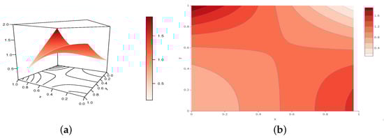
Figure 14. Illustrations of the (a) perspective plot and (b) contour plot of the TGCC copula density for the following configuration: $a=-1/2$, $b=2$, and $c=1$, belonging to Configuration 2.

From these figures, we see how the parameters a, b, and c affect the shapes of the TGCC copula density; the overall shapes between Figure 13 and Figure 14 are really different.

As a last important function, the survival TGCC copula is the function ${\widehat{C}}_3(·;\theta ):I\to [0,1]$ defined by

$$\begin{array}{cc}\hfill & {\widehat{C}}_3(x,y;\theta )=x+y-1+C_3(1-x,1-y;\theta )\hfill \\ \hfill & =x+y-1+(1-x)(1-y)exp\left\{a[1-{(1-x)}^b]y^c\right\},(x,y)\in I.\hfill \end{array}$$

Under Configurations 1 and 2, it defines a legitimate copula and has the same analytical elements as the TGCC copula.

4.3. Key Characteristics

Some key characteristics of the TGCC copula under Configurations 1 and 2 are now discussed.

• The TGCC copula is not symmetric except for the case $a=0$, or $b=c=1$.
• For $a\ne 0$, like the GCC and SGCC copulas, the TGCC copula is not Archimedean.
• For $a\ne 0$, the TGCC copula is not radially symmetric because there exists $(x,y)$ such that ${\widehat{C}}_3(x,y;\theta )\ne C_3(x,y;\theta )$.
• The TGCC copula is positively quadrant dependent for $a\ge 0$ (corresponding to Configuration 1) since $C_3(x,y;\theta )\ge xy$ for any $(x,y)\in I$. It is negatively quadrant dependent for $a<0$ (corresponding to Configuration 2) since $C_3(x,y;\theta )\le xy$ for any $(x,y)\in I$.
• Using the following inequality: $e^u\ge 1+u$ for any $u\in \mathbb{R}$, for any $(x,y)\in I$, we obtain

  $$C_3(x,y;\theta )\ge C_{☆}(x,y;\theta ),$$

  where $C_{☆}(x,y;\theta )=xy\left[1+a(1-x^b){(1-y)}^c\right]$. Hence, for some parameter values, $C_{☆}(x,y;\theta )$ is smaller than $C_3(x,y;\theta )$ with respect to the concordance ordering.
• Using the following inequality: $e^{-u}\ge 1-u$ for any $u\in \mathbb{R}$, for a, b, and c, such that $u=a(1-x^b){(1-y)}^c<1$ for any $(x,y)\in I$, we have

  $$C_3(x,y;\theta )\le C_{▹}(x,y;\theta ),$$

  where

  $$C_{▹}(x,y;\theta )=\frac{xy}{1-a(1-x^b){(1-y)}^c}.$$
  For some values of the parameters, $C_{◃}(x,y;\theta )$ represents a generalized AMH copula. Hence, for some parameter values, $C_3(x,y;\theta )$ is smaller than $C_{◃}(x,y;\theta )$ with respect to the concordance ordering.
• In full generality, there is no concordance ordering between the GCC, SGCC and TGCC copulas.
• The FH bounds hold.
• For $(x,y)\in [0,1]\times [0,1)$, using the exponential series and (standard and generalized) binomial expansions, the TGCC copula can be expressed as

  $$\begin{array}{c}\hfill C_3(x,y;\theta )=\sum _{i=0}^{\infty }\sum _{j=0}^i\sum _{k=0}^{\infty }{\xi }_{i,j,k}{x}^{bj+1}{y}^{k+1},\end{array}$$

  (8)

  where

  $${\xi }_{i,j,k}=\frac{a^i}{i!}\left(\genfrac{}{}{0pt}{}{i}{j}\right)\left(\genfrac{}{}{0pt}{}{ci}{k}\right){(-1)}^{j+k}.$$
  Similarly, the TGCC copula density can be expanded as

  $$c_3(x,y;\theta )=\sum _{i=0}^{\infty }\sum _{j=0}^i\sum _{k=0}^{\infty }{\zeta }_{i,j,k}{x}^{bj}{y}^k,$$

  where ${\zeta }_{i,j,k}=(bj+1)(k+1){\xi }_{i,j,k}$.
• The possible tail dependence of the TGCC copula is now explored. Using standard limit techniques, we have

  $${\lambda }_L=\underset{x\to 0}{lim}\frac{C_3(x,x;\theta )}{x}=\underset{x\to 0}{lim}xexp\left[a(1-x^b){(1-x)}^c\right]=0$$

  and

  $${\lambda }_U=\underset{x\to 1}{lim}\frac{1-2x+C_3(x,x;\theta )}{1-x}=\underset{x\to 1}{lim}\frac{1-2x+x^{2}exp\left[a(1-x^b){(1-x)}^c\right]}{1-x}=0.$$
  Hence, the TGCC copula has no tail dependence.
• The medial correlation of the TGCC copula is given by

  $$M=4C_3\left(\frac{1}{2},\frac{1}{2};\theta \right)-1=exp\left[a(1-2^{-b})2^{-c}\right]-1.$$
  As numerical works, Table 11 and Table 12 show some numerical values of M for $\theta =(\gamma ,1/\gamma ,1/\gamma )$ and $\theta =(-\gamma ,1/\sqrt{\gamma },1/\sqrt{\gamma })$ (rounded to the second decimal), for several values of $\gamma \in (0,1]$, being special examples of Configurations 1 and 2, respectively.
  Table 11. Values of the medial correlation of the TGCC copula for $\theta =(\gamma ,1/\gamma ,1/\gamma )$ and several values of $\gamma \in (0,1]$, belonging to Configuration 1.

  $\gamma$	0.01	0.09	0.17	0.25	0.33	0.41	0.49	0.57	0.65	0.73	0.81	0.89
  M	0	0	0	0.01	0.04	0.06	0.09	0.13	0.16	0.19	0.22	0.25

  Table 12. Values of the medial correlation of the TGCC copula for $\theta =(-\gamma ,1/\sqrt{\gamma },1/\sqrt{\gamma })$ and several values of $\gamma$, belonging to Configuration 2.

  $\gamma$	0.01	0.09	0.17	0.25	0.33	0.41	0.49	0.57	0.65	0.73	0.81	0.89
  M	0	−0.01	−0.03	−0.05	−0.07	−0.09	−0.11	−0.13	−0.15	−0.16	−0.18	−0.2

  These tables show that a moderate amplitude of values can result in a medial correlation that is either negative or positive (here, from $-0.2$ to $0.25$).
• The rho of Spearman of the TGCC copula is defined by

  $$\rho =12{\int }_0^1{\int }_0^1\left[C_3(x,y;\theta )-xy\right]dxdy.$$
  It is evident that it lacks a closed-form expression. However, by using Equation (6), we can expand it as

  $$\rho =12\sum _{i=1}^{\infty }\sum _{j=0}^i\sum _{k=0}^{\infty }{\xi }_{i,j,k}\frac{1}{(bj+2)(k+2)}.$$
  Table 13 and Table 14 determine its numerical values for $\theta =(\gamma ,1/\gamma ,1/\gamma )$ and $\theta =(-\gamma ,1/\sqrt{\gamma },1/\sqrt{\gamma })$ (rounded to the second decimal), for several values of $\gamma \in (0,1]$, being special examples of Configurations 1 and 2, respectively.
  Table 13. Values of the rho of Spearman of the TGCC copula for $\theta =(\gamma ,1/\gamma ,1/\gamma )$ and several values of $\gamma \in (0,1]$, belonging to Configuration 1.

  $\gamma$	0.01	0.09	0.17	0.25	0.33	0.41	0.49	0.57	0.65	0.73	0.81	0.89
  $\rho$	0	0	0.01	0.03	0.06	0.09	0.13	0.17	0.21	0.25	0.29	0.33

  Table 14. Values of the rho of Spearman of the TGCC copula for $\theta =(-\gamma ,1/\sqrt{\gamma },1/\sqrt{\gamma })$ and several values of $\gamma \in (0,1]$, belonging to Configuration 2.

  $\gamma$	0.01	0.09	0.17	0.25	0.33	0.41	0.49	0.57	0.65	0.73	0.81	0.89
  $\rho$	0	−0.01	−0.04	−0.06	−0.09	−0.11	−0.14	−0.16	−0.19	−0.21	−0.24	−0.26

  These tables show that the rho of Spearman of the TGCC copula can have a wide range of amplitudes, from negative to positive (here, from $-0.25$ to $0.33$). The TGCC copula is hence perfect for modeling different types of dependence.
• Let $F\left(x\right)$ and $G\left(x\right)$ be two unidimensional CDFs. Then, under Configurations 1 and 2, we define a new two-dimensional CDF by considering the function $H:I\to [0,1]$ indicated as $H(x,y;\theta )=C_3(F\left(x\right),G\left(y\right);\theta )$. Thus, based on this function, there are an endless number of potential new two-dimensional distributions.

As a last remark, based on Proposition 3 and a basic inversion of the roles of b and c, and those of x and y, it is clear that the two-dimensional function $C_4(·;\theta ):I\to [0,1]$ defined by

$$\begin{array}{c}\hfill C_4(x,y;\theta )=xyexp\left[a{(1-x)}^b(1-y^c)\right],(x,y)\in I,\end{array}$$

where $\theta =(a,b,c)\in {\mathbb{R}}^3$, is a copula for the following parameter configurations (non-overlapping):

Configuration 1:

$a\ge 0$, $b\ge 1$, $c>0$, $ab\le 1$, and $ac\le 1$.

Configuration 2:

$a<0$, $b\ge 1$, $c>0$, and $abc\ge -1$.

The properties already discussed for the TGCC copula can be transferred to this copula with no additional work.

5. Conclusions and Possible Extensions

In this paper, we have emphasized and investigated three new three-parameter copulas that generalize the Celebioglu–Cuadras (CC) copula as described in [17,18]. We have identified the main parameter configurations for which the copula remains valid in the mathematical sense. Surprising phenomena were observed for some negative values of the parameters. Numerical and graphic works illustrated the findings. The main properties of the copulas were described in detail, such as their symmetry, quadrant dependence, various expansions, concordance ordering, tail dependences, medial correlation, and Spearman correlation. Thus, this study has the merit of promoting flexible versions of the CC copula, expanding the copula repertoire in the literature, and making available new dependence models for various data analyses (construction of semiparametric models, regression models, etc.). The practical aspect, however, needs further developments that we will leave for future work. In particular, the balance between complexity and robustness of the proposed copula needs investigation. As another theoretical perspectives, possible higher-dimensional generalized CC copulas, say of dimension n, include those of the following form:

$${\displaystyle C_{†}(\mathbf{x};\theta )=\left[\prod _{i=1}^n{x}_i\right]exp\left[a\prod _{i=1}^n{(1-x_i^{{\delta }_i})}^{d_i(1-{\delta }_i)}\right],}$$

where $\mathbf{x}=(x_1,\dots ,x_n)\in {[0,1]}^n$ and $\theta =(a,d_1,\dots ,d_n)\in {\mathbb{R}}^{n+1}$, and $({\delta }_1,\dots ,{\delta }_n)\in {\{0,1\}}^n$. This general copula form should also be feasible, but further research is needed to establish appropriate parameter values.

References

- Cuadras, C.M. The importance of being the upper bound in the bivariate family. SORT 2006, 30, 55–84. [Google Scholar]
- Durante, F.; Sempi, C. Principles of Copula Theory; CRS Press: Boca Raton, FL, USA, 2016. [Google Scholar]
- Joe, H. Dependence Modeling with Copulas; CRS Press: Boca Raton, FL, USA, 2015. [Google Scholar]
- Nelsen, R. An Introduction to Copulas, 2nd ed.; Springer Science+Business Media, Inc.: Berlin, Germany, 2006. [Google Scholar]
- Roberts, D.J.; Zewotir, T. Copula geoadditive modelling of anaemia and malaria in young children in Kenya, Malawi, Tanzania and Uganda. J. Heal. Popul. Nutr. 2020, 39, 8. [Google Scholar] [CrossRef] [PubMed]
- Safari-Katesari, H.; Samadi, S.Y.; Zaroudi, S. Modelling count data via copulas. Statistics 2020, 54, 1329–1355. [Google Scholar] [CrossRef]
- Shiau, J.-T.; Lien, Y.-C. Copula-based infilling methods for daily suspended sediment loads. Water 2021, 13, 1701. [Google Scholar] [CrossRef]
- Tavakol, A.; Rahmani, V.; Harrington, J., Jr. Probability of compound climate extremes in a changing climate: A copula-based study of hot, dry, and windy events in the central United States. Environ. Res. Lett. 2020, 15, 104058. [Google Scholar] [CrossRef]
- Chesneau, C. A note on a simple polynomial-sine copula. Asian J. Math. Appl. 2022, 2, 1–14. [Google Scholar]
- Chesneau, C. A new two-dimensional relation copula inspiring a generalized version of the Farlie-Gumbel-Morgenstern copula. Res. Commun. Math. Math. Sci. 2021, 13, 99–128. [Google Scholar]
- Chesneau, C. On new types of multivariate trigonometric copulas. AppliedMath 2021, 1, 3–17. [Google Scholar] [CrossRef]
- El Ktaibi, F.; Bentoumi, R.; Sottocornola, N.; Mesfioui, M. Bivariate copulas based on counter-monotonic shock method. Risks 2022, 10, 202. [Google Scholar] [CrossRef]
- Michimae, H.; Emura, T. Likelihood inference for copula models based on left-truncated and competing risks data from field studies. Mathematics 2022, 10, 2163. [Google Scholar] [CrossRef]
- Shih, J.-H.; Konno, Y.; Chang, Y.-T.; Emura, T. Copula-based estimation methods for a common mean vector for bivariate meta-analyses. Symmetry 2022, 14, 186. [Google Scholar] [CrossRef]
- Susam, S.O. Parameter estimation of some Archimedean copulas based on minimum Cramér-von-Mises distance. J. Iran. Stat. Soc. 2020, 19, 163–183. [Google Scholar] [CrossRef]
- Susam, S.O. A new family of archimedean copula via trigonometric generator function. Gazi Univ. J. Sci. 2020, 33, 795–802. [Google Scholar] [CrossRef]
- Celebioglu, S. A way of generating comprehensive copulas. J. Inst. Sci. Technol. 1997, 10, 57–61. [Google Scholar]
- Cuadras, C.M. Constructing copula functions with weighted geometric means. J. Stat. Plan. Inference 2009, 139, 3766–3772. [Google Scholar] [CrossRef]
- Bekrizadeh, H.; Parham, G.; Jamshidi, B. A new asymmetric class of bivariate copulas for modeling dependence. Commun. Stat. Simul. Comput. 2017, 46, 5594–5609. [Google Scholar] [CrossRef]
- Cuadras, C.M.; Diaz, W.; Salvo-Garrido, S. Two generalized bivariate FGM distributions and rank reduction. Commun. Stat. Theory Methods 2020, 49, 5639–5665. [Google Scholar] [CrossRef]
- Manstavičius, M.; Bagdonas, G. A class of bivariate independence copula transformations. Fuzzy Sets Syst. 2022, 428, 58–79. [Google Scholar] [CrossRef]
- Diaz, W.; Cuadras, C.M. An extension of the Gumbel-Barnett family of copulas. Metrika 2022, 85, 913–926. [Google Scholar] [CrossRef]
- Huang, J.S.; Kotz, S. Modifications of the Farlie-Gumbel-Morgenstern distributions. a tough hill to climb. Metrika 1999, 49, 135–145. [Google Scholar] [CrossRef]
- Choros, B.; Ibragimov, R.; Permiakova, E. Copula estimation. In Copula Theory and Its Applications; Lecture Notes in Statistics; Springer: Berlin/Heidelberg, Germany, 2010; Volume 198, pp. 77–91. [Google Scholar]
- Joe, H. Multivariate Models and Dependence Concepts, Monographs on Statistics and Applied Probability; Chapman & Hall/CRC: New York, NY, USA, 2001; Volume 73. [Google Scholar]
- Taketomi, N.; Yamamoto, K.; Chesneau, C.; Emura, T. Parametric distributions for survival and reliability analyses, a review and historical sketch. Mathematics 2022, 10, 3907. [Google Scholar] [CrossRef]
Disclaimer/Publisher’s Note: The statements, opinions and data contained in all publications are solely those of the individual author(s) and contributor(s) and not of MDPI and/or the editor(s). MDPI and/or the editor(s) disclaim responsibility for any injury to people or property resulting from any ideas, methods, instructions or products referred to in the content. |
© 2023 by the author. Licensee MDPI, Basel, Switzerland. This article is an open access article distributed under the terms and conditions of the Creative Commons Attribution (CC BY) license (https://creativecommons.org/licenses/by/4.0/).