Abstract
Kidney cancer has become a major global health issue over time, showing how early detection can play a very important role in mediating the disease. Traditional histological image analysis is recognized as the clinical gold standard for diagnosis, although it is highly manual and labor-intensive. Due to this issue, many are interested in computer-aided diagnostic technologies to assist pathologists in their diagnostics. Specifically, deep learning (DL) has become a viable remedy in this field. Nonetheless, the capacity of existing DL models to extract comprehensive visual features for accurate classification is limited. Toward the end, this study proposes using ensemble models that combine the strengths of multiple transformers and deep learning model architectures. By leveraging the collective knowledge of these models, the ensemble enhances classification performance and enables more precise and effective kidney cancer detection. This study compares the performance of these suggested models to previous studies, all of which used the publicly accessible Dartmouth Kidney Cancer Histology Dataset. This study showed that the Vision Transformers, with an average accuracy of over 99%, were able to achieve high detection accuracy across all complete slide picture patches. In particular, the CAiT, DeiT, ViT, and Swin models outperformed ResNet. All things considered, the Vision Transformers consistently produced an average accuracy of 98.51% across all five-folds. These results demonstrated that Vision Transformers might perform well and successfully identify important features from smaller patches. Through utilizing histopathological images, our findings will assist pathologists in diagnosing kidney cancer, resulting in early detection and increased patient survival rates.
1. Introduction
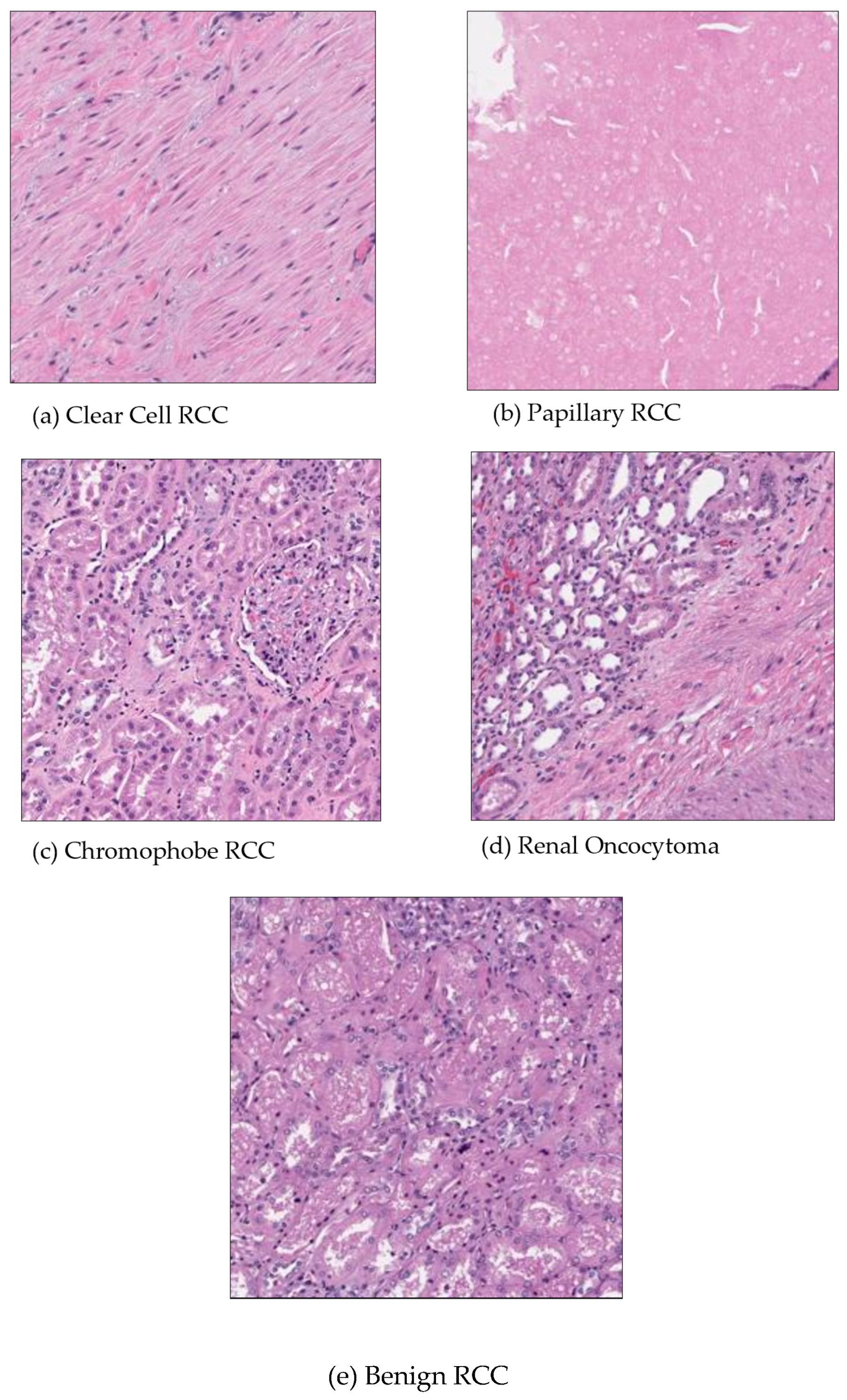
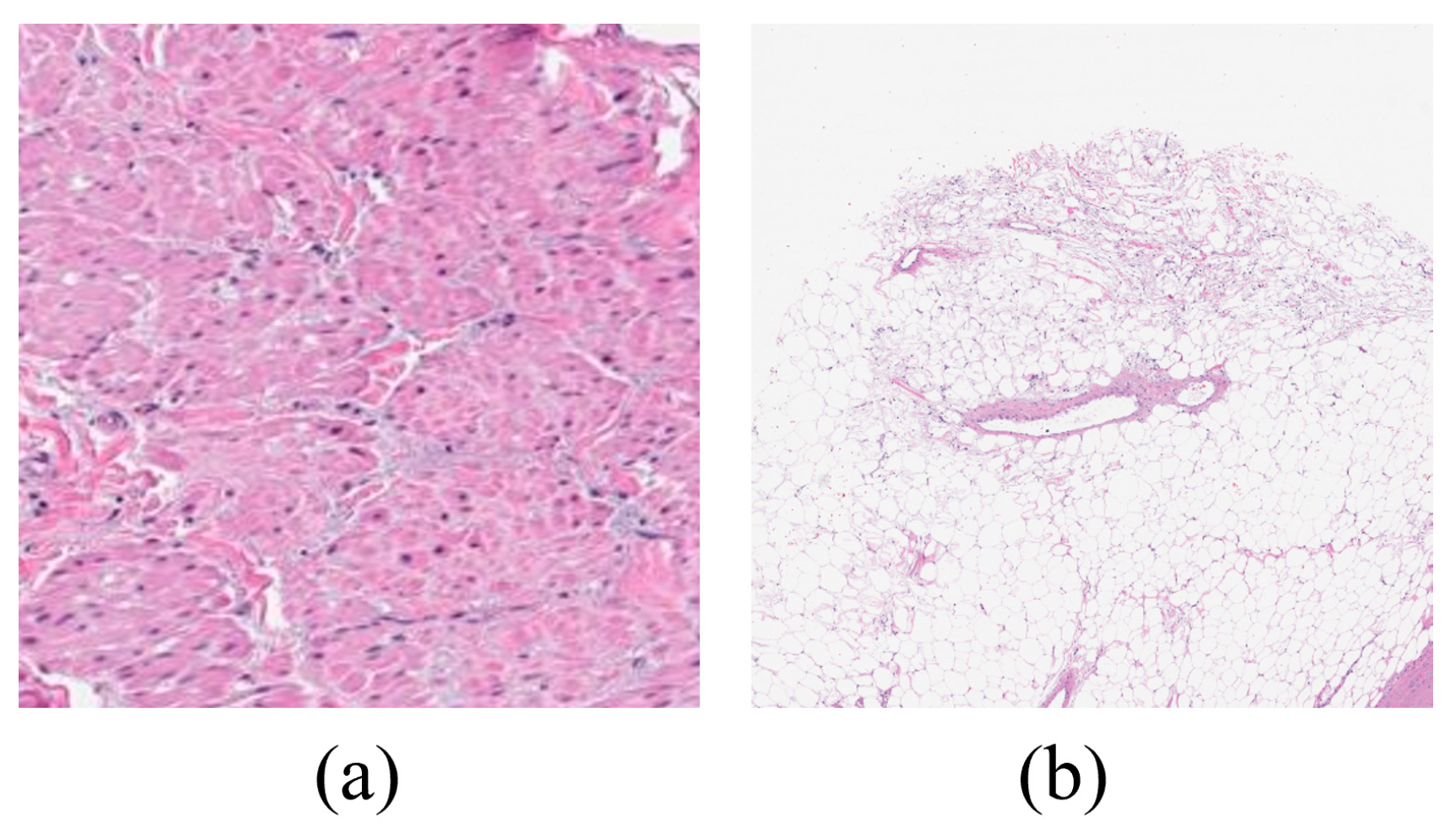
Patients with renal cancer frequently exhibit symptoms such as anemia and fever which can lower blood cancer levels and lead to poor red blood cell counts. The most common harmful subtype of renal cancer is clear cell renal carcinoma [Figure 1a]. The stroma of these tumors is highly vascular, which often leads to hemorrhagic regions. The characteristic yellow appearance of the tumor surface is due to the lipid composition of the cells, which includes high levels of cholesterol, neutral lipids, and phospholipids. Roughly 10% of renal cell carcinomas are papillary renal cell carcinomas [Figure 1b]. Recent studies have demonstrated the potential of digital pathology and deep learning in cancer diagnosis. Kondejkar et al. (2024) achieved high accuracy in prostate cancer grading using multi-scale digital pathology and deep learning. Similarly, Balasubramanian et al. (2024) employed ensemble deep learning techniques for breast cancer subtype and invasiveness diagnosis, achieving impressive classification accuracies. These advancements provide a strong foundation for applying similar approaches to kidney cancer diagnosis using the Dartmouth Kidney Cancer Histology Dataset [1,2]. Like clear cell renal cell carcinoma, papillary renal cell carcinoma has an age distribution with a reported mean age at diagnosis typically ranging from 50 to 65 years. Necrosis is a common feature of papillary renal cell carcinomas [3,4,5]. About 5% of renal cancers are chromophobe renal cell carcinomas. Their prognosis is better than that of clear cell kidney carcinoma. The death rate is under 10%. There have been cases of chromophobe renal carcinoma that have distantly metastasized to the pancreas, liver, and lung. It has been proposed that chromophobe renal tumors have a higher incidence of liver metastasis than other histological subtypes [6,7] [Figure 1c]. Renal oncocytoma is a benign tumor, and it is believed to be the precursor of eosinophilic chromophobe renal cell carcinoma, which is the malignant variant of this tumor [Figure 1d]. Benign kidney cancer can manifest in several forms including renal clear cell, papillary, chromophore, oncocytoma, and benign [Figure 1].
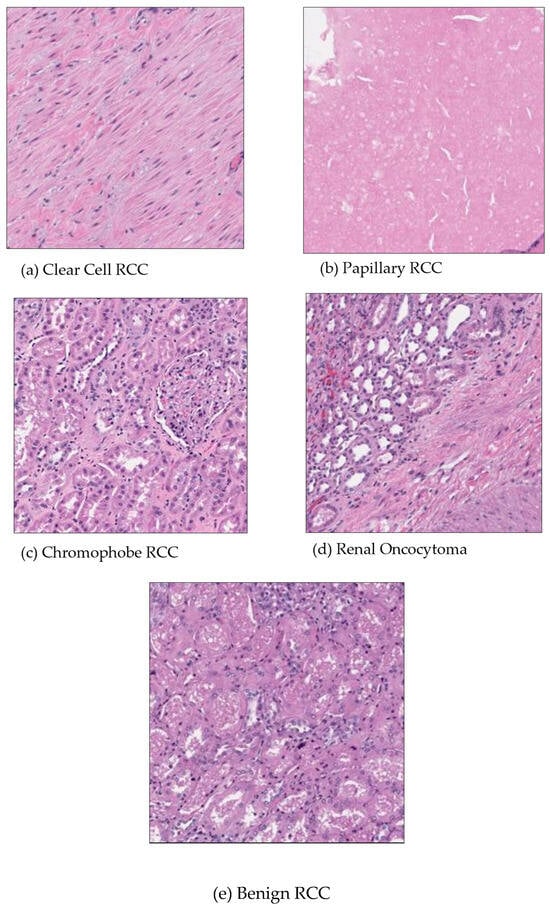
Figure 1.
An example of microscopy images for five classes in Dartmouth Kidney Cancer Histology Dataset (on 40× magnification).
Bone metastases occur in about one-third of patients with advanced renal cell carcinoma (RCC), causing significant morbidity. These predominantly osteolytic metastases can lead to severe complications such as pain, fractures, and spinal cord compression, greatly impacting patients’ quality of life and prognosis [8]. RCCs (renal cell carcinomas) typically do not cause any symptoms until late in the course of the illness, and more than 50% of tumors are discovered by chance [9]. Merely 10 to 15% of patients can exhibit the “classic triad”, which consists of flank fullness, hematuria, and discomfort.
The experience and expertise of the pathologist plays a major role in the accuracy of the histopathological analysis, which leaves the manual method open to human error including improper diagnosis and detection. Additionally, a lack of pathologists causes major delays in the examination of patient cases, which may result in the diagnosis of cancer later than expected [10,11]. Zhou et al. (2018) developed a deep learning-based radiomics model to distinguish benign from malignant renal tumors using medical imaging, demonstrating its potential to improve diagnostic accuracy and aid clinical decision-making (Zhou et al., 2018) [12].
The three main components of the proposed CAD system as described by Shehata et al. [13] are the preprocessing of gray images to create 3D segmented objects representing renal tumors; extracting various discriminating features (texture and functional) from segmented objects; and completing a two-stage classification process using various machine learning classifiers to determine the renal tumor final diagnosis [13]. Texture analysis is frequently utilized to give multiple quantitative patterns or descriptors that may be obtained by linking the gray values of each pixel in each tumor image or volume during the process of obtaining discriminating features.
2. Materials and Methods
2.1. Literature Review
There are imaging techniques such as CT (Computed Tomography) and MRI (Major Research Instrumentation) that can detect tumors or abnormal growths in the kidneys. Blood and urine tests are also conducted to identify the features linked to kidney cancer. The identification and categorization of kidney cancer has made great progress in recent years because of the application of deep learning techniques. By combining radiomic characteristics and clinical data, a multimodal deep-learning system was developed that achieved a 94% accuracy rate in the early diagnosis of kidney cancer disease. To classify kidney cancers in MRI scans, Chen used transfer learning with pre-trained VGG-16 and ResNet-50 models, obtaining accuracies of 87% and 89%, respectively. Using a modified U-Net architecture, Gao achieved 90% classification accuracy and 91% segmentation accuracy when they categorized renal cell carcinoma in histopathological pictures. Additionally, Nguyen obtained a Dice coefficient of 0.89 and a classification accuracy of 92%, demonstrating the efficacy of a combined CNN-RNN strategy for segmenting and categorizing renal masses. These findings demonstrate the revolutionary potential of deep learning to improve the precision and efficacy of kidney cancer diagnosis, opening the door to more dependable and individualized treatment approaches. The paper by Breggie presents a web app using AI and multimodal data to improve prostate cancer diagnosis. Users valued its summary tabs and high-resolution images. This study suggests improvements while highlighting the app’s potential to enhance diagnostic accuracy and efficiency.
Originally, hand-crafted features like color, texture, and morphology were extracted from histopathology pictures and used to identify kidney cancer using classic machine learning (ML) methods including support vector machines (SVM), random forests, and Ada boost. Compared to manual analysis, these techniques significantly improved results, producing more reliable and consistent outcomes. For example, Zhou achieved a noteworthy accuracy of 88% by using a mix of color and texture information in a random forest classifier to identify between benign and malignant kidney cancers. Deep learning’s introduction has completely changed the field of digital pathology. Convolutional neural networks (CNNs) have proven to be incredibly effective at tasks like cancer-related histopathology, image recognition, and segmentation. CNNs are especially useful for medical image analysis since they can automatically learn hierarchical feature representations from raw pixel data. Research has demonstrated that CNNs are as accurate as human pathologists, if not more so, in certain areas, including determining the severity of a tumor and recognizing malignant tissues. Esteva, for instance, showed that a CNN could classify skin cancer with dermatologist-level accuracy [14]. This discovery has now been applied to other cancer types, such as kidney cancer. Agrawal and Juneja (2019) explored deep learning models for medical image analysis, highlighting key challenges and future research directions, emphasizing their transformative potential in healthcare (Agrawal & Juneja, 2019) [15].
A study by Jiang assessed the suggested models using the recently released Dartmouth Kidney Cancer Histology Dataset [16] to determine their effectiveness. Ivanova reviewed AI models for renal cell carcinoma (RCC) diagnosis using the histological image dataset, highlighting high accuracies in classification and grading tasks. Convolutional neural networks (CNNs) and deep learning models often exceed 90% accuracy, with one CNN achieving 99.1% accuracy in RCC tissue identification. Other effective approaches include Bayesian classifiers and support vector machines. These AI techniques show significant potential for improving RCC diagnosis and management in clinical practice.
This study’s primary contributions are the creation of transformer models and an efficient deep ensemble learning model that outperforms existing research on the Kidney Cancer Histology Dataset for kidney cancer detection. Moreover, the successful identification of kidney histology patches by the ensemble model of Swin and Vision Transformer may lead to a reduction in the number of digital scanners, data storage devices, and computer servers required for histopathology-related tasks. This has the potential to improve patient survival rates and raise the likelihood of renal or kidney cancer being detected early [13,16].
2.2. Dataset Description
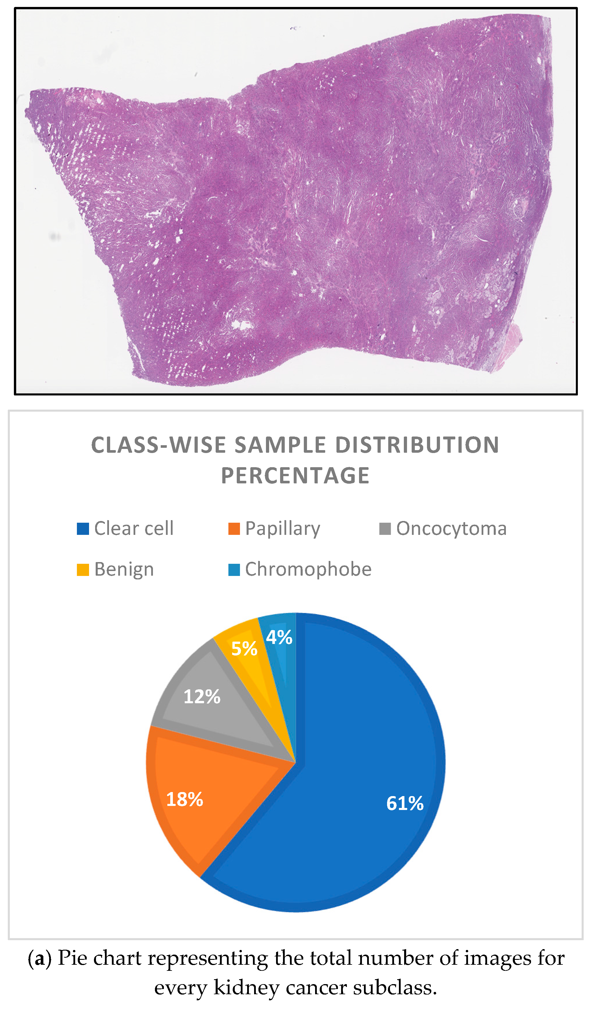
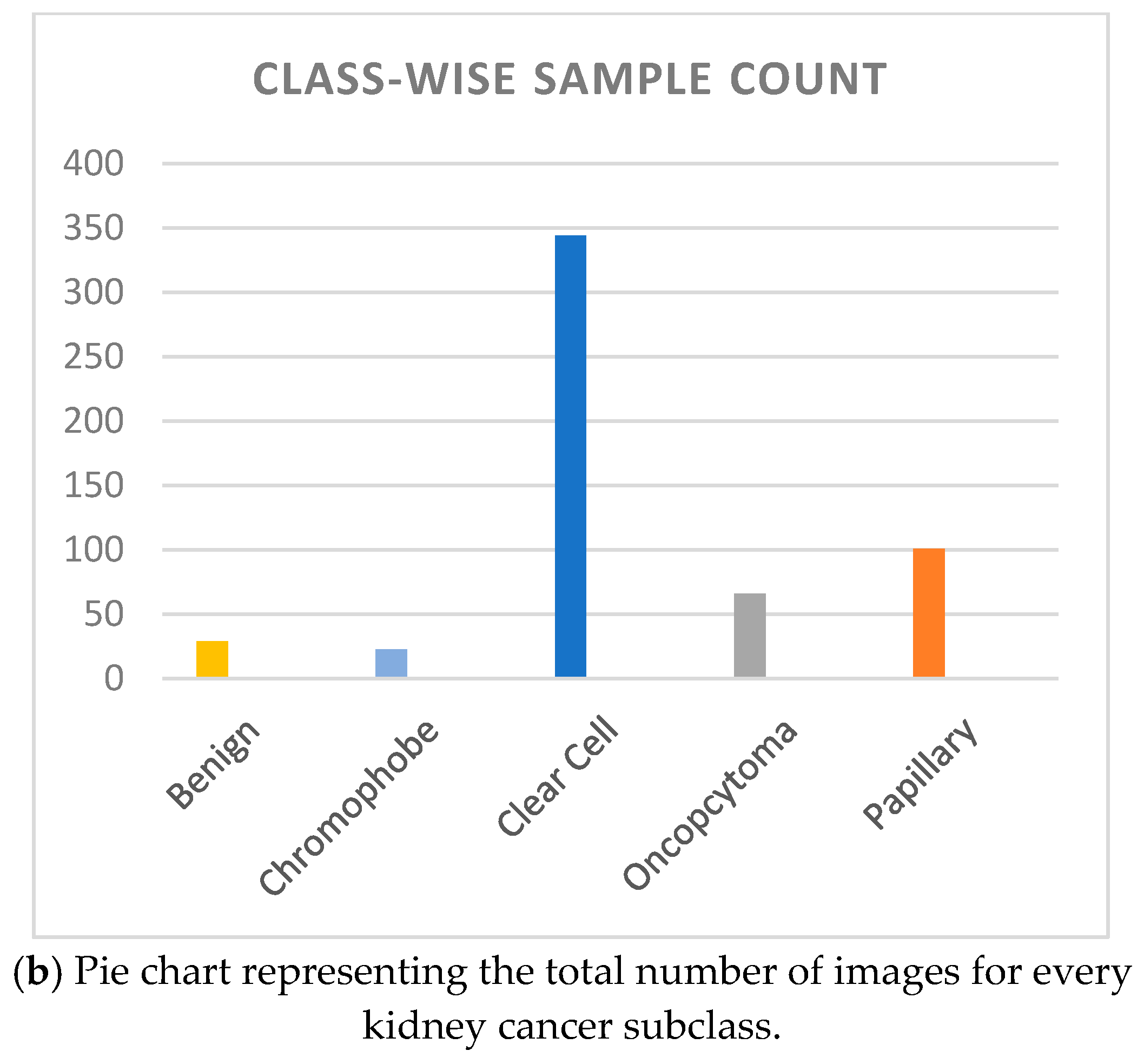
The Dartmouth Kidney Cancer Histology Dataset (Supplementary Materials) is a large collection of 563 whole-slide images (WSIs) [Figure 2a] stained with hematoxylin and eosin (H&E) that have been carefully chosen for analysis and kidney cancer. The images provide a broad dataset that is essential for research in digital pathology and machine learning applications in medical diagnostics. The dataset includes a wide range of kidney cancer subtypes, including oncocytoma, chromophobe renal cell carcinoma (chRCC), papillary renal cell carcinoma (pRCC), and clear cell renal cell carcinoma (ccRCC). To properly categorize and diagnose kidney tumors, machine learning models need to be trained with these as labels. The dataset includes metadata including the file name, image class, slide type, and split type (Train, Test, and Val), in addition to various demographic data. Understanding the context of each histopathology image and performing in-depth analysis is facilitated with this information. In particular, the dataset is useful for creating and comparing computer-aided diagnostic (CAD) systems. It offers a wealth of data for deep learning models and other machine learning algorithms to improve their performance in kidney cancer diagnosis and classification. Additionally, it facilitates clinical decision-making by offering a point of reference for the confirmation and comparison of diagnostic results [Figure 2].

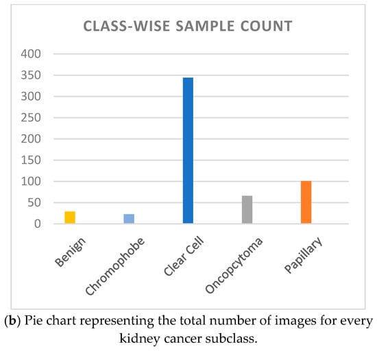
Figure 2.
Example of histopathological kidney cancer whole-slide images.
2.3. Methodology Overview
This study demonstrates the use of Vision Transformer techniques with CNN architectures to identify kidney cancer patches. There are four main steps in the process: First, the dataset is created by removing empty patches and augmenting it. Next, pre-trained networks or base models are tailored. Third, the most successful base models are selected to generate ensemble models. Finally, the models are evaluated and presented using various metrics and the class activation map.
The ensemble model approach is a key feature of this study, combining the strengths of Vision Transformers (ViTs) and Swin Transformer architectures. This ensemble strategy leverages the complementary capabilities of both models, with the ViT excelling in capturing global image context and the Swin Transformer adept at handling multi-scale feature hierarchies. By averaging the outputs of these two powerful models, the ensemble achieves a synergistic effect, enhancing overall classification accuracy and robustness. The ensemble model demonstrated exceptional performance, achieving a remarkable accuracy of 99.26% in classifying kidney cancer histology images.
Data preprocessing was performed to improve the model’s performance by deleting non-informative empty patches from the dataset. These patches would have biased the training process and compromised the model’s performance. Following the elimination of empty patches, data augmentation was used to expand the training dataset.
The ensemble model was designed to leverage the complementary strengths of the ViT and Swin Transformer. The ViT excels at capturing global image features through its self-attention mechanism, while the Swin Transformer captures hierarchical and local features via its sliding window approach. The final ensemble combines their outputs using a weighted averaging strategy, where weights were optimized through cross-validation. This approach ensures a balance of local and global feature representations, leading to superior performance.
2.4. Empty Patch Removal Process
This study focuses on the efficient management and processing of whole-slide images (WSIs) for patch extraction using OpenSlide Library. The main goal is to eliminate empty patches, defined as those with over half of pixels having RGB intensity values greater than 230 in all channels. OpenSlide, an open-source C library, is used to read and modify digital pathology images. The implementation involves using OpenSlide to read WSIs and tools from the tools package for tissue detection and patch extraction. The process includes setting up paths, reading metadata, and using a Tissue Detector class with a Gaussian Naive Bayes model for tissue recognition. A Patch Extractor class is employed with specific parameters to extract relevant patches. The workflow is optimized through parallel processing using Python’s multiprocessing package, resulting in an efficient and transparent approach for managing WSIs and extracting valuable data for further analysis. With this process, every high-resolution image is broken into different patches depending on the RGB intensity, and the ensemble models are trained on them [Figure 3]. Goode et al. introduced OpenSlide, a vendor-neutral software platform for digital pathology, enabling standardized and scalable analysis of pathology images (Goode et al., 2013). He et al. (2016): He et al. proposed Deep Residual Learning (ResNet), a groundbreaking architecture for image recognition, which addressed the vanishing gradient problem and achieved state-of-the-art performance (He et al., 2016) [17,18].
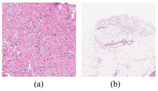
Figure 3.
The pictures above exhibit examples of histopathology: (a) tissue patch image and (b) empty patch image.
2.5. Pre-Trained Networks as Base Models
Since the beginning of deep learning, convolutional neural networks (CNNs) have been helpful in many applications because of their constant improvements in strength, efficiency, and adaptability. CNNs, which are specifically designed for computer vision problems and use convolutional layers inspired by natural visual processes, are a great example of this innovation. The accuracy, speed, and overall performance of various CNN structures have improved over time, and they are frequently compared to the ImageNet project—a sizable visual database that fosters advances in computer vision.
In the past, training CNNs from scratch took a lot of time and computer power. By using previously learned information from trained models, transfer learning (TL) offers a useful shortcut that can speed up optimization and possibly increase classification accuracy. TL entails transferring weights from pre-trained models, using insights acquired from varied datasets, and speeding training processes to improve model accuracy, particularly in complicated architectures.
2.5.1. ResNet50 Architecture
Deeper than ResNet34, ResNet50 is a 50-layer variant of the ResNet architecture. While this increased depth can lead to better performance on some tasks, training with it requires more processing power. By enabling gradients to flow across shortcut connections, ResNet50, a deep convolutional neural network with 50 layers, introduces the idea of residual learning and helps to address the disappearing gradient issue. This design is efficient in several computer vision applications, most notably picture categorization [Figure 4].
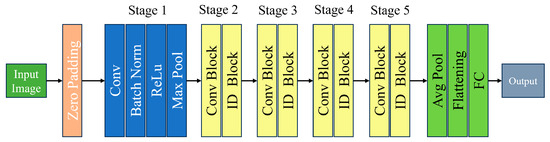
Figure 4.
ResNet50 model architecture.
2.5.2. Transformers
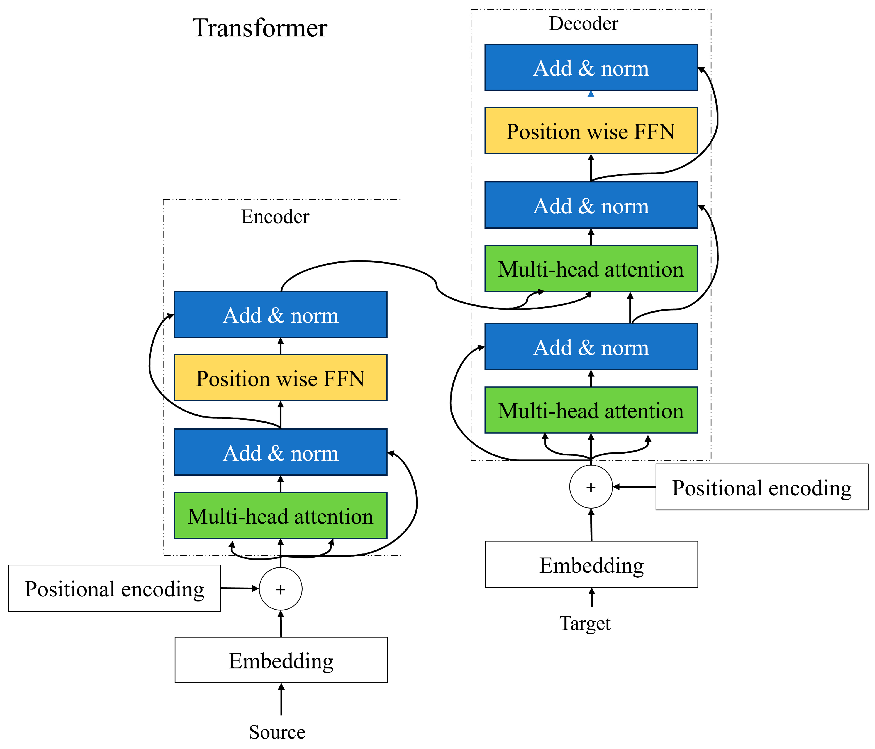
Transformers are network models that use attention to understand the sequence of information like frames in a movie, words in a sentence, notes in music, or pixels of an image. The transformer networks can capture relationships and dependencies between the elements even if they are far apart from each other. The ability to capture long-range dependencies makes transformers powerful for tasks like language understanding where the meaning of the words depends on words that appear earlier or later in the sentence. The transformer network consists of two main parts: (1) encoder; and (2) decoder.
2.5.3. Encoder and Decoder
The input sequence that we achieve from positional encoding is passed through the encoder. Each encoder consists of a self-attention mechanism and a feed-forward neural network to capture the contextual information and dependencies between the words. The multi-head attention layer helps the model to figure out which words are important to each other and how they relate to one another. In the self-attention layer, each word will have three jobs such as query, key, and value. A query is a word looking for other words to pay attention to. The key is a word being looked at by other words. The self-attention layer looks at each word and compares it with all other words in the sentence and sees how they are related to each other. It calculates the similarity between each word query and all word keys. The words with the higher scores will be prioritized. The add and norm layer is applied after the multi-headed attention layer and feed-forward neural network in each transformer network. It preserves the original information from the previous layer, which allows the model to learn and update the new information captured by the sublayer. It assists in addressing the vanishing gradient problems and allows the model to learn more effectively [Figure 5].
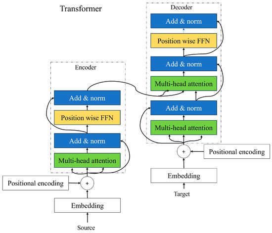
Figure 5.
Architecture of encoder and decoder of transformer.
The primary function of the decoder is to transform encoded representations back into the desired output format. In sequence generation tasks like machine translation and text summarization, the decoder predicts the next token in the sequence at each time step, often utilizing techniques like beam search to improve output quality. In data reconstruction applications, such as image or audio reconstruction, the decoder transforms encoded latent representations back into the original data format, a common approach in autoencoders and generative models like Variational Autoencoders (VAEs) and Generative Adversarial Networks (GANs). Additionally, decoders are designed for conditional output production, where the output is conditioned on additional context or input data, and for error correction and denoising, where they reconstruct clean data from noisy inputs.
The decoder is integral to various neural network architectures, especially in sequence-to-sequence models and data reconstruction tasks. It typically includes an embedding layer, recurrent layers, attention mechanisms, transformer layers, and an output layer. These components collaboratively transform encoded representations into meaningful outputs. The decoder’s primary functions include sequence generation, data reconstruction, conditional output production, and error correction. Transformer-based decoders utilize self-attention, cross-attention, and feed-forward networks for enhanced performance. Applications of decoders span natural language processing, computer vision, speech processing, and healthcare, highlighting their versatility and importance in modern neural network models. Understanding their architecture and functions is essential for optimizing data transformation tasks.
2.5.4. CAiT Architecture (Class Attention in Image Transformers)
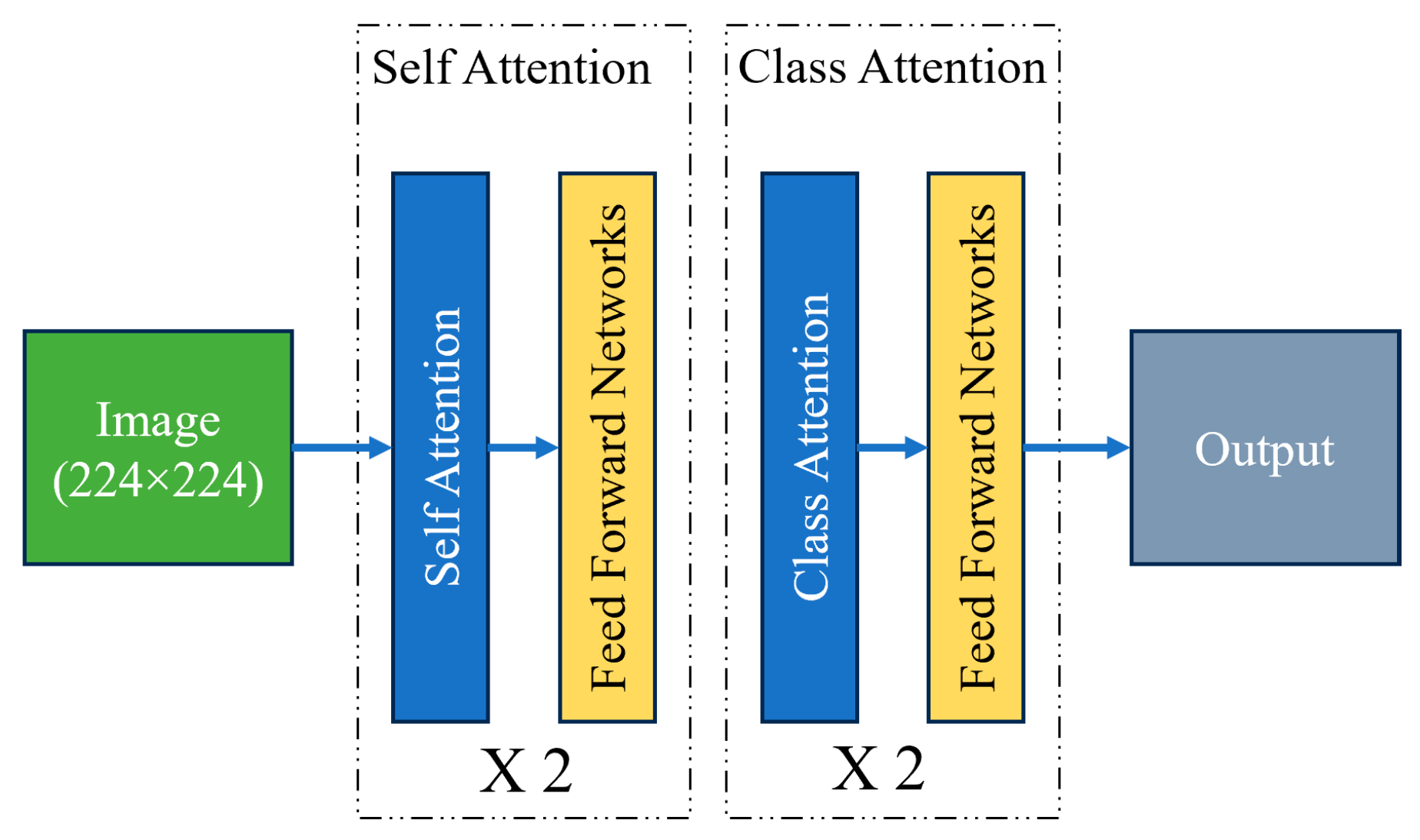
The CAiT (class-attention in Image Transformers) transformer is a novel architecture designed to enhance the performance of Vision Transformers (ViTs) in image classification tasks. Traditional Vision Transformers apply self-attention mechanisms uniformly across all patches of an input image, which can sometimes lead to the suboptimal learning of class-specific features. CAiT introduces a unique class-attention mechanism that focuses on improving the interaction between class tokens and image patches, leading to better representation learning and classification accuracy. In the CAiT architecture, a class token is appended to the sequence of image patches, and attention is specifically directed toward this class token. This design allows the model to aggregate and emphasize class-specific information more effectively. The class-attention mechanism is integrated at multiple stages of the transformer, enhancing the model’s ability to capture and utilize discriminative features necessary for accurate classification. Additionally, CAiT incorporates deeper transformer layers and a progressive learning approach, gradually increasing the model’s complexity and capacity. This results in improved convergence and performance on various image recognition benchmarks, making CAiT a powerful architecture for vision tasks [Figure 6].
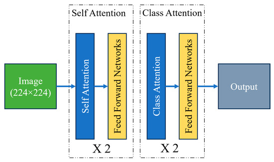
Figure 6.
CAiT transformer architecture.
2.5.5. VitNet Architecture
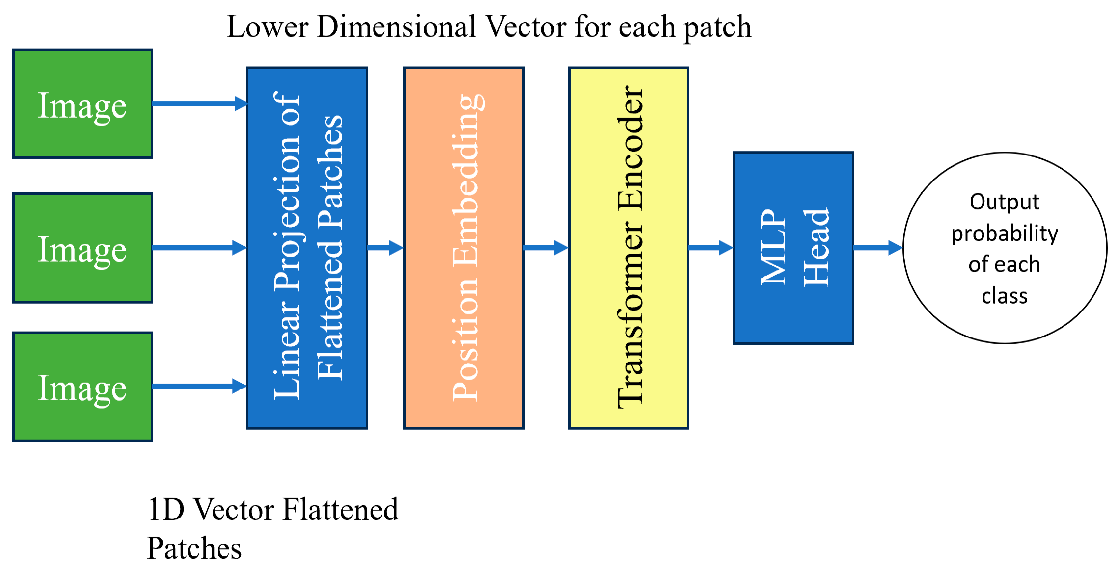
Vision Transformers use self-attention. It allows the model to understand the relationship between different parts of an image by assigning important scores to patches and focusing on the most relevant information. This helps the model make better sense of the image and perform various tasks related to computer vision. It breaks images into smaller patches [19]. The statement used in the paper ‘An image is worth 16 × 16 words’ means how many pixels the sliding window moves each time. Each patch is treated as a separate input token. There is no decoder in the vision transformer, it is an encoder-only transformer. Linear projection works on flattened patches by transforming 1D vectors into a lower-dimensional representation. It preserves the important features [Figure 7].
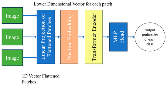
Figure 7.
VITNet model architecture.
2.5.6. DeiT Architecture
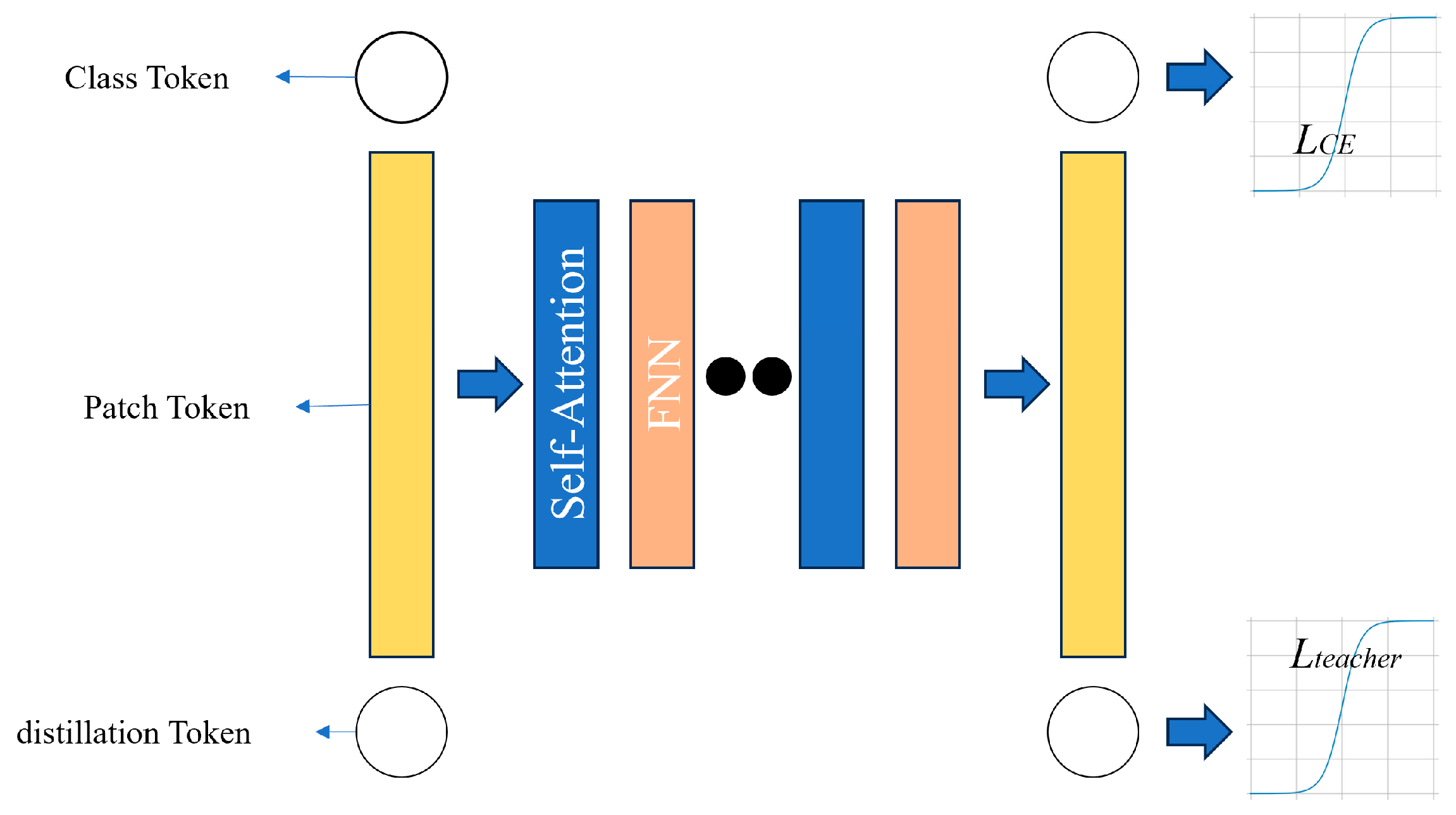
The difference between the ViT and DeiT is that originally the ViT was trained on a massive dataset having 300 M samples of data [20]. The DeiT on the other hand, trains on well-known ImageNet Dataset. The ViT takes a long time to become trained whereas the DeiT trains in 2 or 3 days on a single 8GPU or 4GPU machine. The DeiT uses knowledge distillation which means transferring knowledge from one model/network to another. Regularization is used which means the overfitting of a network is being reduced to limited training data so that the model does not learn the noise from the training data but the actual information from the data. Augmentation is when multiple samples are created of the same input with some variations. Suppose there is a model which classifies cats and dogs. We pass the cat image through the model and obtain the embeddings of the image. The embeddings are passed through self max function to obtain the probabilities of the dog and cat. Cross-entropy loss is compared with the ground-truth label and the entire function. With distillation, we distill the knowledge from another network called the teacher network, we obtain the embeddings and pass it through self-max with the temperature parameter to obtain the output probabilities so that it becomes smoothened [Figure 8].
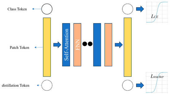
Figure 8.
DeiT model architecture.
2.5.7. Swin Architecture
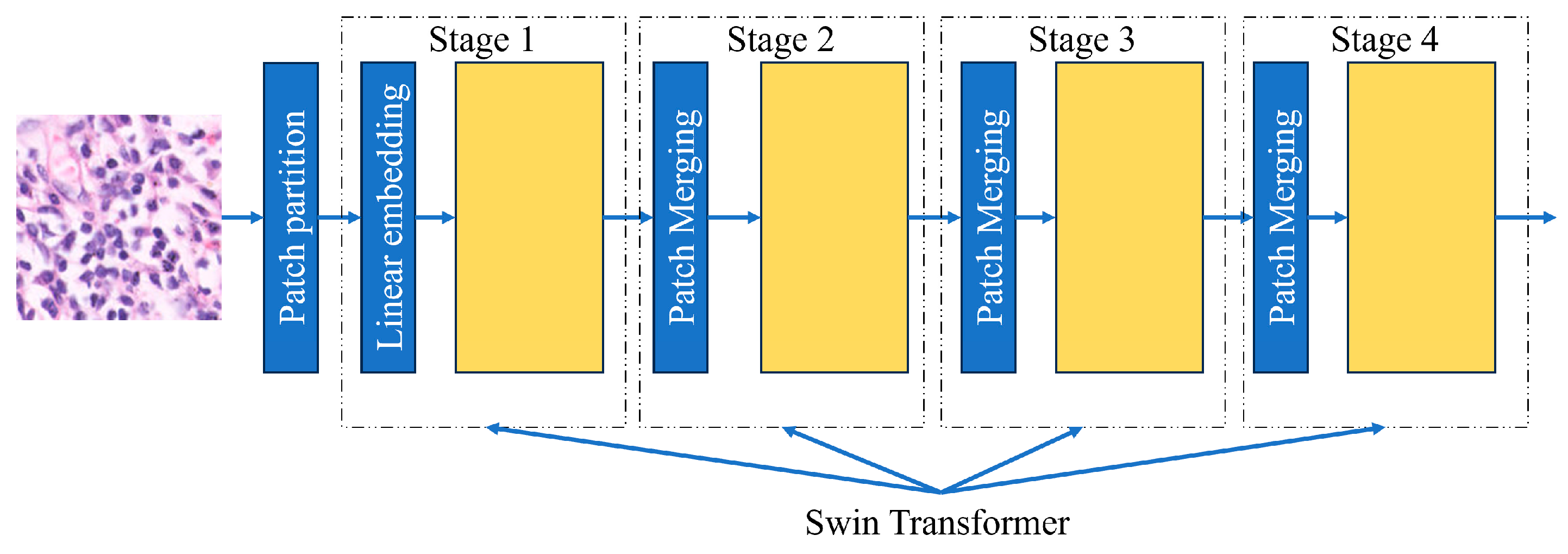
Swin Transformers are more accurate than Vision Transformers in some cases due to their capacity to handle large images and high-resolution images with lower computational complexity. The Swin Transformer, or Shifted Window Transformer, enhances traditional Vision Transformers by targeting their limitations in image processing and the process by which they do it. It is constructed as a hierarchical design with shifted windows, enabling efficient and scalable visual data modeling. Instead of using the whole-slide image all at once, it is divided into different sections. The model looks at the relationship between all the features and then analyzes the section. These windows or sections are shifted across all layers so that they can make connections with different features of the image. This method shows that the Swin Transformer can detect images with accuracy [Figure 9].
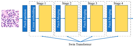
Figure 9.
Diagram showing Swin Transformer architecture.
In this research, CNN model architecture and Vision Transformers were used. Initially, each model was trained independently to determine its unique performance. Then, the best-performing epochs for each model were based on validation accuracy.
To improve the robustness and generalizability of the techniques, 5-fold cross-validation was used. During each fold of the cross-validation approach, the research utilized the average calculation of the last epoch of every fold to calculate the best-performing validation accuracy.
2.6. Experimental Setting
The data were divided into training and validation sets. Each network was trained for 12 epochs using 5-fold cross-validation to create the model. The weights from the epoch with the best validation accuracy were chosen as the final representations for each model. Various metrics were then employed to assess accuracy, followed by many objective assessment factors to determine overall performance.
3. Results
The performance evaluation criteria used include validation accuracy and the Validation Cohen Kappa Score. Positive samples include abnormal or malignant patches, whereas negative samples contain normal or healthy patches. The phrases true positive (TP), false positive (FP), true negative (TN), and false negative (FN) are used to describe the various prediction results.
1. Train loss: A machine learning model’s fit to the training set of data are shown by its train loss. On the training dataset, it measures the difference between the expected and actual outputs. Reducing this loss is the goal of training to enhance the model’s functionality.
2. Validation loss: A machine learning model’s ability to generalize to previously unknown data is measured by the validation loss. On the validation dataset, it measures the difference between the expected and actual outputs.
3. Validation accuracy means the ratio of correctly predicted instances out of the total number of instances in the validation dataset. It is computed as follows:
4. Validation Cohen Kappa Score is a statistical measure.
A complete view of the model’s performance, especially in differentiating between positive and negative data, can be obtained by looking at these metrics.
Performance metrics must be considered while evaluating the efficacy of machine learning models. These metrics offer quantifiable figures that represent a statistical or machine learning technique’s overall performance. Performance metrics assess the model’s ability to consistently produce the correct classifications and its ability to classify data points accurately in classification tasks. The table below displays the study’s conclusions, which were arrived at by looking at various performance criteria [Table 1].

Table 1.
The effectiveness of the several deep learning models was assessed as displayed below.
4. Discussion
In this study, we successfully implemented an ensemble of deep learning and transformer models to classify kidney cancer histopathology images, achieving great validation accuracy rates. Our ensemble, which included ViT and Swin models, demonstrated that this ensemble model can detect critical features from histopathological images. The ensemble model’s approach of processing images as grids of patches facilitates the effective diagnosis of images, which was crucial in achieving the highest validation accuracy of 99.26% and less training loss as well. These results highlight the potential of combining Vision Transformers and Swin Transformers in digital pathology, offering a significant improvement relative to traditional convolutional neural network models such as ResNet and Vgg 16.
Moreover, our research demonstrates the potential of these advanced models to enhance diagnostic accuracy and efficiency in clinical settings. The consistent performance of Vision Transformers and Swin Transformers across the five kidney cancer types—benign, chromophobe, clear cell, oncocytoma, and papillary—demonstrates their robustness. This could lead to the earlier and more accurate detection diagnosis of kidney cancer, improving patient and doctor report outcomes. By taking into consideration the strengths of both Swin Transformers and Vision Transformers, our ensemble approach not only provides a good diagnostic tool but also paves the way for future research in the application of advanced deep learning models in medical image analysis. The successful implementation and high performance of these models suggest a promising direction for integrating AI-based solutions into routine pathological workflows.
Due to limited access to independent kidney cancer histology datasets, this study primarily focused on the Dartmouth Kidney Cancer Histology Dataset. However, the dataset diversity in staining and imaging conditions provides robust evaluations. Future work will include external validation using datasets obtained through collaborations with other institutions to assess the model’s generalization capabilities comprehensively.
Future Directions
This study highlights important directions for enhancing kidney cancer diagnosis through digital pathology and deep learning. The main areas for improvement include the integration of medical reports and X-ray scans. This paper and study emphasize the importance of AI tools that can detect the accuracy and the type of image easily just by seeing the image. By harnessing the full potential of AI-driven digital pathology and web tools to detect the type of cancer in the images by uploading the cancer image, this research paves the way for more accurate, efficient, and reliable diagnostic tools using deep learning models in oncology. Singh et al. (2023) developed an AI-based web application for enhancing prostate cancer diagnosis by integrating deep learning models, multimodal data, and feedback from usability studies with pathologists, demonstrating improved diagnostic workflows (Singh et al., 2023) [21].
5. Conclusions
This study of kidney cancer diagnosis shows the effectiveness of deep learning and ensemble transformer models in classifying kidney cancer histopathology images, with a focus on comparing their performance on metrics such as validation accuracy, validation Cohen Kappa Score, training loss, and validation loss. Our analysis reveals that the ensemble model of the Vision Transformer and the Swin Transformer and Vision Transformers alone, particularly the ViTNet model, excel in identifying critical features from histopathological images, with the highest validation accuracy of 99.26% achieved by the ensemble of the Swin and Vision Transformers. The improvement in accuracy across various models signifies the potential of the ensemble transformer to outperform convolutional neural network models.
The performance of the models trained along five different kidney types shows the robustness of those models in clinical applications such as the application of detecting kidney cancer. The integration of AI can also be made so that the use cases can be extended in other domains as well. By reducing the errors, this application can be used in many different domains by various kinds of people. Our findings show precise use cases where such a study will be very helpful in clinical domains.
Supplementary Materials
The Kidney Cancer Dataset is openly available at this link: https://bmirds.github.io/KidneyCancer/. (Access Date: 20 June 2024).
Author Contributions
Conceptualization, S.M.A.A.-H. and S.A.; Methodology, M.N.J., J.R.A., S.M.A.A.-H. and S.A.; Software, M.N.J., J.R.A., S.M.A.A.-H. and S.A.; Validation, S.A., M.N.J., S.M.A.A.-H., J.R.A. and S.A.; Formal analysis, S.A.; Investigation, S.M.A.A.-H. and S.A.; Writing—original draft, M.N.J.; Writing—review & editing, S.M.A.A.-H., J.R.A. and S.A.; Visualization, S.A.; Supervision, S.A. All authors have read and agreed to the published version of the manuscript.
Funding
This research received no funding.
Institutional Review Board Statement
Not applicable.
Informed Consent Statement
Not applicable.
Data Availability Statement
The data presented in this study are available in this article.
Acknowledgments
We would like to express our deepest gratitude to the Roux Institute, the IEAI, and the Alfond Foundation for their invaluable support and contributions.
Conflicts of Interest
The authors declare no conflicts of interest.
References
- Moch, H. An overview of renal cell cancer: Pathology and genetics. Semin. Cancer Biol. 2012, 23, 3–9. [Google Scholar] [CrossRef] [PubMed]
- Moch, H.; Gasser, T.; Amin, M.B.; Torhorst, J.; Sauter, G.; Mihatsch, M.J. Prognostic utility of the recently recommended histologic classification and revised TNM staging system of renal cell carcinoma: A Swiss experience with 588 tumors. Cancer 2000, 89, 604–614. [Google Scholar] [CrossRef] [PubMed]
- Mudavadkar, G.R.; Deng, M.; Al-Heejawi, S.M.A.; Arora, I.H.; Breggia, A.; Ahmad, B.; Christman, R.; Ryan, S.T.; Amal, S. Gastric Cancer Detection with Ensemble Learning on Digital Pathology: Use Case of Gastric Cancer on GasHisSDB Dataset. Diagnostics 2024, 14, 1746. [Google Scholar] [CrossRef] [PubMed]
- Thoenes, W.; Störkel, S.; Rumpelt, H.J. Human chromophobe cell renal carcinoma. Virchows Arch. B Cell Pathol. Incl. Mol. Pathol. 1985, 48, 207–217. [Google Scholar] [CrossRef]
- Thoenes, W.; Störkel, S.; Rumpelt, H.; Moll, R.; Baum, H.P.; Werner, S. Chromophobe cell renal carcinoma and its variants report on 32 cases. J. Pathol. 1988, 155, 277–287. [Google Scholar] [CrossRef] [PubMed]
- Amin, M.B.; Crotty, T.B.; Tickoo, S.K.; Farrow, G.M. Renal Oncocytoma: A Reappraisal of Morphologic Features with Clinicopathologic Findings in 80 Cases. Am. J. Surg. Pathol. 1997, 21, 1–12. [Google Scholar] [CrossRef] [PubMed]
- Luciani, L.G.; Cestari, R.; Tallarigo, C. Incidental renal cell carcinoma-age and stage characterization and clinical implications: The study of 1092 patients (1982–1997). Urology 2000, 56, 58–62. [Google Scholar] [CrossRef] [PubMed]
- Chen, S.C.; Kuo, P.L. Bone Metastasis from Renal Cell Carcinoma. Int. J. Mol. Sci. 2016, 17, 987. [Google Scholar] [CrossRef] [PubMed]
- Pandey, J.; Syed, W. Renal Cancer. In StatPearls [Internet]; StatPearls Publishing: Treasure Island, FL, USA, 2024. Available online: https://www.ncbi.nlm.nih.gov/books/NBK558975/ (accessed on 8 August 2023).
- Zhou, L.; Zhang, Z.; Chen, Y.-C.; Zhao, Z.-Y.; Yin, X.-D.; Jiang, H.-B. A Deep Learning-Based Radiomics Model for Differentiating Benign and Malignant Renal Tumors. Transl. Oncol. 2018, 12, 292–300. [Google Scholar] [CrossRef]
- MShehata, M.; Alksas, A.; Abouelkheir, R.T.; Elmahdy, A.; Shaffie, A.; Soliman, A.; Ghazal, M.; Abu Khalifeh, H.; Razek, A.A.; El-Baz, A. A New Computer-Aided Diagnostic (Cad) System For Precise Identification Of Renal Tumors. In Proceedings of the 2021 IEEE 18th International Symposium on Biomedical Imaging (ISBI), Nice, France, 13–16 April 2021; pp. 1378–1381. [Google Scholar] [CrossRef]
- Esteva, A.; Kuprel, B.; Novoa, R.A.; Ko, J.; Swetter, S.M.; Blau, H.M.; Thrun, S. Dermatologist-level classification of skin cancer with deep neural networks. Nature 2017, 542, 115–118. [Google Scholar] [CrossRef] [PubMed]
- Agrawal, R.K.; Juneja, A. Deep Learning Models for Medical Image Analysis: Challenges and Future Directions. In Big Data Analytics; BDA 2019; Lecture Notes in Computer Science; Madria, S., Fournier-Viger, P., Chaudhary, S., Reddy, P., Eds.; Springer: Cham, Switzerland, 2019; Volume 11932. [Google Scholar] [CrossRef]
- Jiang, S.; Hondelink, L.; Suriawinata, A.A.; Hassanpour, S. Masked pre-training of transformers for histology image analysis. J. Pathol. Inform. 2024, 15, 100386. [Google Scholar] [CrossRef]
- Goode, A.; Gilbert, B.; Harkes, J.; Jukic, D.; Satyanarayanan, M. OpenSlide: A vendor-neutral software foundation for digital pathology. J. Pathol. Inform. 2013, 4, 27. [Google Scholar] [CrossRef]
- He, K.; Zhang, X.; Ren, S.; Sun, J. Deep Residual Learning for Image Recognition. In Proceedings of the IEEE Conference on Computer Vision and Pattern Recognition (CVPR), Las Vegas, NV, USA, 27–30 June 2016; pp. 770–778. [Google Scholar]
- Han, K.; Wang, Y.; Chen, H.; Chen, X.; Guo, J.; Liu, Z.; Tang, Y.; Xiao, A.; Xu, C.; Xu, Y.; et al. A Survey on Vision Transformer. IEEE Trans. Pattern Anal. Mach. Intell. 2023, 45, 87–110. [Google Scholar] [CrossRef] [PubMed]
- Liu, Z.; Lin, Y.; Cao, Y.; Hu, H.; Wei, Y.; Zhang, Z.; Lin, S.; Guo, B. Swin Transformer: Hierarchical Vision Transformer using Shifted Windows. In Proceedings of the 2021 IEEE/CVF International Conference on Computer Vision (ICCV), Montreal, QC, Canada, 10–17 October 2021; pp. 9992–10002. [Google Scholar] [CrossRef]
- Singh, A.; Randive, S.; Breggia, A.; Ahmad, B.; Christman, R.; Amal, S. Enhancing Prostate Cancer Diagnosis with a Novel Artificial Intelligence-Based Web Application: Synergizing Deep Learning Models, Multimodal Data, and Insights from Usability Study with Pathologists. Cancers 2023, 15, 5659. [Google Scholar] [CrossRef] [PubMed] [PubMed Central]
- Ivanova, E.; Fayzullin, A.; Grinin, V.; Ermilov, D.; Arutyunyan, A.; Timashev, P.; Shekhter, A. Empowering Renal Cancer Management with AI and Digital Pathology: Pathology, Diagnostics and Prognosis. Biomedicines 2023, 11, 2875. [Google Scholar] [CrossRef] [PubMed] [PubMed Central]
- Liu, W.; Qiu, J.-L.; Zheng, W.-L.; Lu, B.-L. Comparing Recognition Performance and Robustness of Multimodal Deep Learning Models for Multimodal Emotion Recognition. IEEE Trans. Cogn. Dev. Syst. 2022, 14, 715–729. [Google Scholar] [CrossRef]

Disclaimer/Publisher’s Note: The statements, opinions and data contained in all publications are solely those of the individual author(s) and contributor(s) and not of MDPI and/or the editor(s). MDPI and/or the editor(s) disclaim responsibility for any injury to people or property resulting from any ideas, methods, instructions or products referred to in the content. |
© 2025 by the authors. Licensee MDPI, Basel, Switzerland. This article is an open access article distributed under the terms and conditions of the Creative Commons Attribution (CC BY) license (https://creativecommons.org/licenses/by/4.0/).