Statistical Analysis of Ceiling and Floor Effects in Medical Trials

Abstract

Exploratory data analysis and statistical moments were used to investigate the potential impact of ceiling and floor effects in medical trials. A total of 150 treatment-naive eyes were assessed in a retrospective case study of patients who were treated with anti-VEGF injections for wet age-related macular degeneration. The experimental results revealed that ceiling and floor effects are problematic in data analysis and may result in serious errors when using standard parametric tests. The case study provided insights relating to methodology in medical trials, experimental data analysis, and statistical inference, as applied to the interpretation of treatment response limits. Suggestions are provided for statistical data pre-processing and post-processing when significantly skewed distributions are present in response groups.

1. Introduction

Age-related macular degeneration (AMD) is a progressive, clinically heterogeneous eye disease that is most prevalent in the ageing population (i.e., 60 years or older) [1,2]. It is a leading cause of central vision deterioration and blindness [3,4,5]. Due to the growth of the aging population, the prevalence of AMD is also increasing [6], and it affects millions of aging individuals worldwide, with its prevalence predicted to increase dramatically [4,7,8].

The disease affects a small region approximately 2 mm in diameter in the central part of the retina known as the macula [6]. The macula is responsible for discerning fine details and is required for simple tasks such as reading, recognising faces, and driving [9]. The patients become co-dependent on the acuity of their peripheral vision to compensate for the lack of central vision [8].

The pathology of early AMD is distinguishable by the presence of drusen: focal whitish-yellow lipids that are found between the retinal pigment epithelium (RPE) and Bruch’s membrane [10,11]. While drusen occur naturally as part of the aging process, their presence may accumulate progressively and increase the risk of the advanced forms of AMD [7,12,13]. AMD is composed of two advanced types: non-exudative (dry) AMD and exudative (wet) AMD [14,15]. The advanced forms of AMD are characterised by either damage or loss of photoreceptors, degeneration of RPE cells within the macular region, or the formation of new vessels from the underlying choroid [2,16]. The majority of severe vision loss occurs in the wet AMD form. In 2011, Deloitte reported that 51,709 patients across Australia suffered from severe wet AMD, while 8,843 suffered from severe dry AMD [5,17].

At present, treatment is available for wet AMD and a number of companies have provided a range of products that have now become widely used by clinicians. Currently, treatments for wet AMD include anti-vascular endothelial growth factor (anti-VEGF) options such as ranibizumab (Lucentis^®, Genentech Inc., San Francisco, CA, USA), bevacizumab (Avastin^®, Genentech Inc., San Francisco, CA, USA), and aflibercept (Eylea^®, Regeneron Pharmaceuticals Inc., Tarrytown, NY, USA). These anti-VEGF agents are injected intravitreally to limit the progression of choroidal neovascularization associated with neovascular AMD [18]. These intravitreal injections have largely superseded older treatments, such as photodynamic therapy and laser photocoagulation, which were less effective and had less predictable outcomes [17,19]. The aim of the AMD-targeted therapies is to arrest the progression of the disease and improve vision. Patients are categorised into one of three treatment groups based on their response profile: responders (improved vision), stable responders (little or no change in vision), and non-responders (vision deterioration). Approximately 10–20% of patients have been reported in some studies as being non-responders [20].

It has been suggested that responders are limited in their progress by the phenomenon known as the “ceiling effect”, while non-responders are affected by the “floor effect” [21]. The ceiling effect refers to the upper-most extreme end point in any group or dataset. The floor effect, conversely, occurs at the lowest end of the scale range. In the context of AMD, the ceiling effect refers to the greatest level of improvement a patient can achieve over the course of their treatment. According to the ceiling effect, anything beyond that threshold is unattainable. It is anticipated that non-responders will decline continually until they reach severe vision loss or blindness.

When the ceiling or floor effect occurs in a group, information is lost regarding the true differences between individuals [22]. If the individual patient responses are the same, it is not possible to correlate differences with a range of possible predictors [23].

Ceiling and floor effects can also occur in randomised clinical trials and can have potentially significant impacts when comparing the mean response between a test group and control group, possibly invalidating the study altogether [24]. In a medical study, a ceiling or floor effect may appear in the treatment group as a narrow clustering of responses at either end of the measurement scale, characterised by skewness in the statistical distribution of responses.

This study was conducted to test for the presence of ceiling and floor effects in response groups and to identify their potential impacts and importance in data analysis. The study investigated patients treated with anti-VEGF injections in a retrospective case study comparing three groups: responders, non-responders, and stable responders. The statistical analysis described can be generalised to apply to randomised controlled trials with active, placebo, and control arms [24].

2. Materials and Methods

2.1. Study Design and Eligibility

The retrospective case study was based on anonymised data from a cohort of patients who attended the Royal Victorian Eye and Ear Hospital (RVEEH) between 2006 and 2010. The data provided comprehensive statistics for technical analysis.

2.2. Patient Selection

The cohort consisted of 150 treatment-naive eyes, with patients >50 years of age and diagnosed with subfoveal choroidal neovascularization (CNV) secondary to AMD. Patients were diagnosed by retinal specialists experienced in the management of AMD. Clinical diagnoses were based on retinal examinations, fundus photography, fundus fluorescein angiography, and time-domain optical coherence tomography (OCT) with Stratus OCT version 5.0.1 (Carl Zeiss Meditec, Dublin, CA, USA) or Cirrus HD-OCT version 6.0.0.599 (Carl Zeiss Meditec). Visual acuity (VA) scores were obtained using the Early Treatment Diabetic Retinopathy Study (ETDRS) chart performed at 4 metres. The presence of intra-retinal fluid (IRF), sub-retinal fluids (SRF), macular thickness, macular scar, atrophy, and haemorrhage were analysed using OCT. These variables were collected for baseline, 3-, 6-, 12-, and 24-month treatment intervals.

Not included were patients with CNV secondary to non-AMD conditions such as angioid streaks, severe myopia, central serous retinopathy, or hereditary retinal disorders and those who received any previous treatment for neovascular AMD such as an anti-VEGF, photodynamic therapy, or laser treatment.

2.3. Treatment and Response Profiles

The patients were treated with either ranibizumab or bevacizumab. A total of 140 patients were treated for either the left eye (LE) or the right eye (RE) (i.e., 140 eyes). Five patients were treated for both eyes (i.e., 10 eyes). Patients were treated with monthly injections during the first three months of therapy. After the third month, injection intervals were determined using the inject-and-extend protocol. This protocol involves the modification of the treatment intervals in accordance with a patient’s progress. If the patient responds well, the time between each injection was extended by two weeks. For example, a patient on monthly injections may then proceed to receive injections every six weeks. The maximum allowable interval is 12 weeks. Non-responders continue to receive monthly injections.

The patients were classified into three groups as follows. Responders were characterised by an improved VA score of at least 5 letters and the presence or absence of IRF/SRF, macular thickness, haemorrhage, etc. Patients that had a loss of at least 5 letters, fluid present, and recurrent retinal haemorrhage were deemed non-responders. Patients with a change in VA between −4 and 4 letters were classified as stable responders.

2.4. Statistical Analysis

The variability in patient response was investigated by conducting Exploratory Data Analysis (EDA), which was pioneered by Tukey [25]. The objectives of EDA include the following [26]:

(a)

Providing insights into data characteristics, features, and patterns.

(b)

Producing graphical representations of data for the purpose of visualisation.

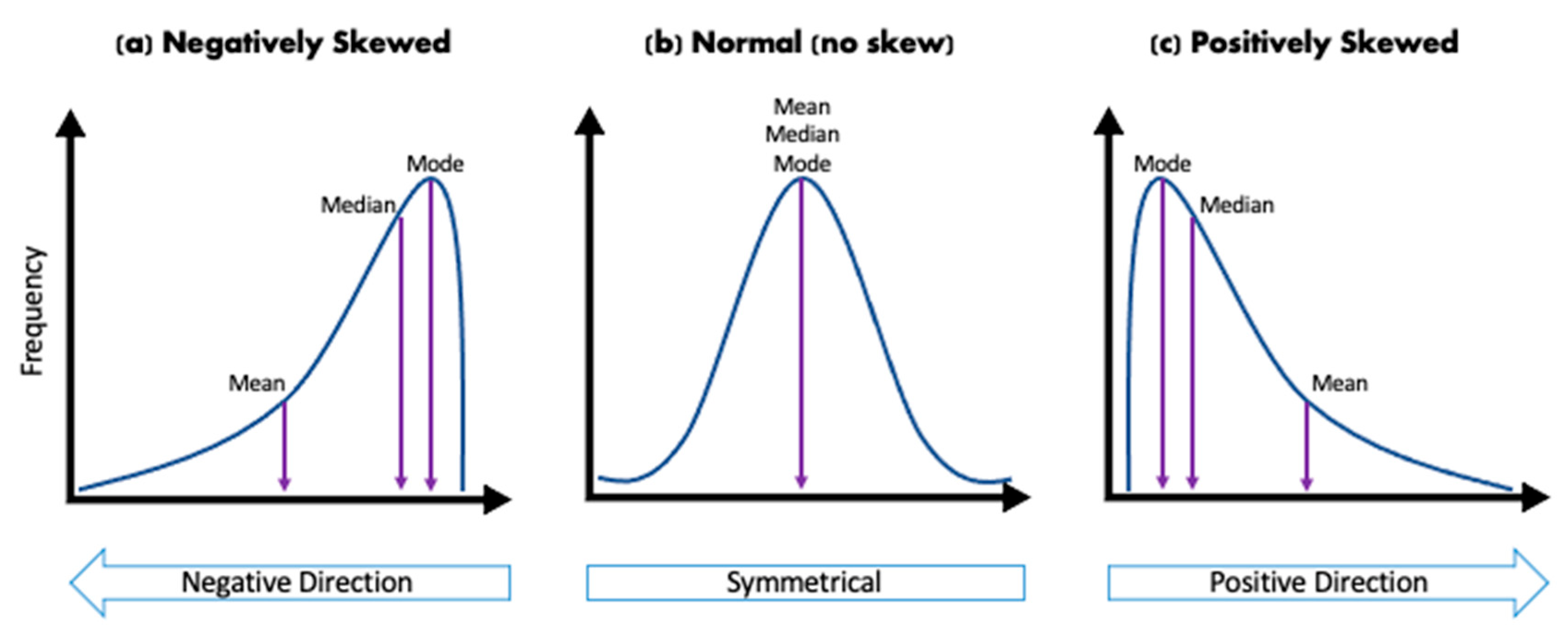
The EDA was used to analyse patient responses to treatment and interpret ceiling and floor effects in the data in the context of wet AMD treatment response. Ceiling and floor effects represent a clustering of data at each end of the measurement scale. A quantitative indicator of clustering at the extremes of the measurement scale is skewness in the statistical distribution of the data [27,28].

To verify the presence of skewness, data were reviewed using visualisation techniques, such as scatterplots, box plots, and histograms, and basic skewness metrics. A ceiling effect for an individual is associated with the maximum achievable vision response observed following a number of injections. In pharmacology, it reflects the fact that, after a number of treatments with a drug, there is often a diminishing effect with time and convergence to a limiting value.

In a clinical trial, a ceiling effect may manifest itself as extreme skewness in the statistical distribution of the responses from patients (Figure 1a). The ceiling effect refers to strong skewness to the left, i.e., negative skew [27]. In this case, most patient responses are strongly above the mean response and tightly clustered with minimal dispersion. This can be interpreted as the dose being large enough to affect all patients in a similar manner in the sample. Conversely, the floor effect refers to strong skewness to the right, i.e., positive skew (Figure 1c). In this case, most patient responses are well below the mean and tightly clustered with minimal dispersion. This can be interpreted as the dose being too small to have any significant effect on most patients.

In principle, the skewness metric may approach a limiting value (corresponding to either ceiling or floor) whereby all the patients are either at the floor (with minimum or zero response, with no dispersion) or alternatively at a ceiling with maximum response, with no dispersion. In such an extreme case, there is no ranking of patients or correlation possible with any potential predictors of anti-VEGF response. The ideal case is when there is no skewness, as represented by a normal distribution (Figure 1b).

In other words, for a group of patients, the ceiling effect and floor effect relate to clustering of patient responses around a particular response level at each end of the scale. Thus, ceiling effects can occur when a very significant proportion of patients achieve the best or maximum possible response, and the floor effect is the opposite, i.e., when a very significant proportion achieve the lowest or minimum response.

The poor data quality resulting from ceiling and floor effects can have a significant impact on the derivation of predictive models because there is a lack of correlation between the treatment response and predictors, including old age, obesity, or smoking status (that is, the correspondence between predictors and response may be “many-to-one” rather than the desirable “one-to-one” relationship). Moreover, the poor data quality and low variability can also make statistical inference difficult when using parametric tests to compare treatment and control groups because they assume normal distributions. The issue of data quality will also have an impact on the application of machine learning algorithms for prediction and classification because the algorithms need to be trained on statistical samples that should be accurate, without errors if possible, or duplications, and representative of the broader population, otherwise the prediction accuracy will be diminished [23,24].

Skewness is characterised in terms of the second and third moments around the mean of a statistical distribution [28]. In other words,

$$m_2=\frac{1}{n}\sum _{i=1}^n{\left(x_i-\overline{x}\right)}^2 \mathrm{and} m_3=\frac{1}{n}\sum _{i=1}^n{\left(x_i-\overline{x}\right)}^3$$

(1)

$m_2$ and $m_3$ represent the moments, whereas $x_i$ refers to an $i$th value, and $\overline{x}$ represents the mean. The skewness is usually measured using the traditional Fisher–Pearson Coefficient of Skewness.

$$g_1=\frac{m_3}{m_2^{\frac{3}{2}}}=\frac{\frac{1}{n}\sum _{i=1}^n{\left(x_i-\overline{x}\right)}^3}{{\left[\frac{1}{n}\sum _{i=1}^n{\left(x_i-\overline{x}\right)}^2\right]}^{3/2}}$$

(2)

The distribution of VA scores and OCT changes were reviewed for all patients. The trajectory of response was first reviewed for all patients and then for the individual subgroups of responders, non-responders, and stable responders. Central tendency, skewness, kurtosis, and descriptive statistics were reviewed for quantitative VA scores. The progression of disease for all three response groups using OCT data was analysed with the use of bar plots, as these variables were categorical.

The skewness $g_1$ is a measure of asymmetry in the statistical distribution around its mean value, with a value of zero for the normal probability distribution. There is a wide range of ${|g}_1|$ values quoted in the scientific literature on the limiting value of the skewness level that is acceptable for the normal approximation to be retained.

A common rule of thumb that is often used is the following:

• If ${|g}_1|>1,$ the statistical distribution is highly skewed.
• If 0.5 < ${|g}_1|<1,$ the statistical distribution is moderately skewed.
• If ${|g}_1|<0.5,$ the statistical distribution is approximately symmetrical.

In the last case, the approximation of normality of the statistical distribution is often assumed so that parametric tests of statistical significance can be used on the data. Some authors have suggested a more relaxed standard and cite ${|g}_1|<2$ for satisfying the normality approximation [29,30]. It is noteworthy that increasing degrees of skewness introduce increasing errors in the application of parametric tests. For highly skewed distributions, the arithmetic mean is no longer an appropriate measure of central tendency.

3. Results

3.1. Summary Statistics

The summary statistics for the entire dataset provide demographic information for the patient population, including disease progression, and the overall response to anti-VEGF treatments ranibizumab and bevacizumab over the course of 24 months (

Table 1. Summary statistics: patient demographics and baseline characteristics. Adapted from Ref. [23].

Sex, n (%)
Female	85 (56.7)
Male	65 (43.3)
Age (yrs)
Mean ± SD	78.9 ± 7.3
Range	54–102
Baseline VA, LE
Mean ± SD	53.5 ± 24.0
Range	0–88
Baseline VA, RE
Mean ± SD	48.4 ± 24.3
Range	2–90
Treatment Administered, n (%)
Ranibizumab	122 (81.3)
Bevacizumab	28 (18.7)
Smoking Status, n (%)
No	53 (35.3)
Yes—Past	64 (42.7)
Yes—Present	19 (12.7)
Yes—Virtually Never	8 (5.3)
Missing	6 (4.0)
Smoker Packs (years)
Mean ± SD	39.1 ± 28.7
Range	2–126
Treated Eye, n (%)
LE	64 (42.7)
RE	86 (57.3)
Hypertension, n (%)
No	48 (32)
Yes	102 (68)
Diabetes, n (%)
No	118 (78.7)
Yes	25 (16.7)
Missing	7 (4.6)

). The dataset was not filtered into the three treatment categories during the summary statistics analysis (i.e., responder, non-responder, and stable response).

The cohort of 150 eyes consisted of 85 (56.7%) females and 65 (43.3%) males. The mean age with standard deviation (SD) at baseline was 78.9 ± 7.3 years. The mean baseline VA for the LE was 53.5 ± 24.0 letters, while the RE was 48.4 ± 24.3. Ranibizumab was the primary treatment used, with 122 (81.3%) patients being treated with the anti-VEGF at baseline, while bevacizumab accounted for 28 (18.7%) patient treatments.

Out of all treated eyes, most patients were treated for the RE, with 86 (57.3%) patients being treated for the RE, while 64 (42.6%) were treated for the LE. We found that 10 (6.7%) of the patients were treated for both the LE and RE. A total of 102 (68%) patients had hypertension, and 25 (16.7%) had diabetes.

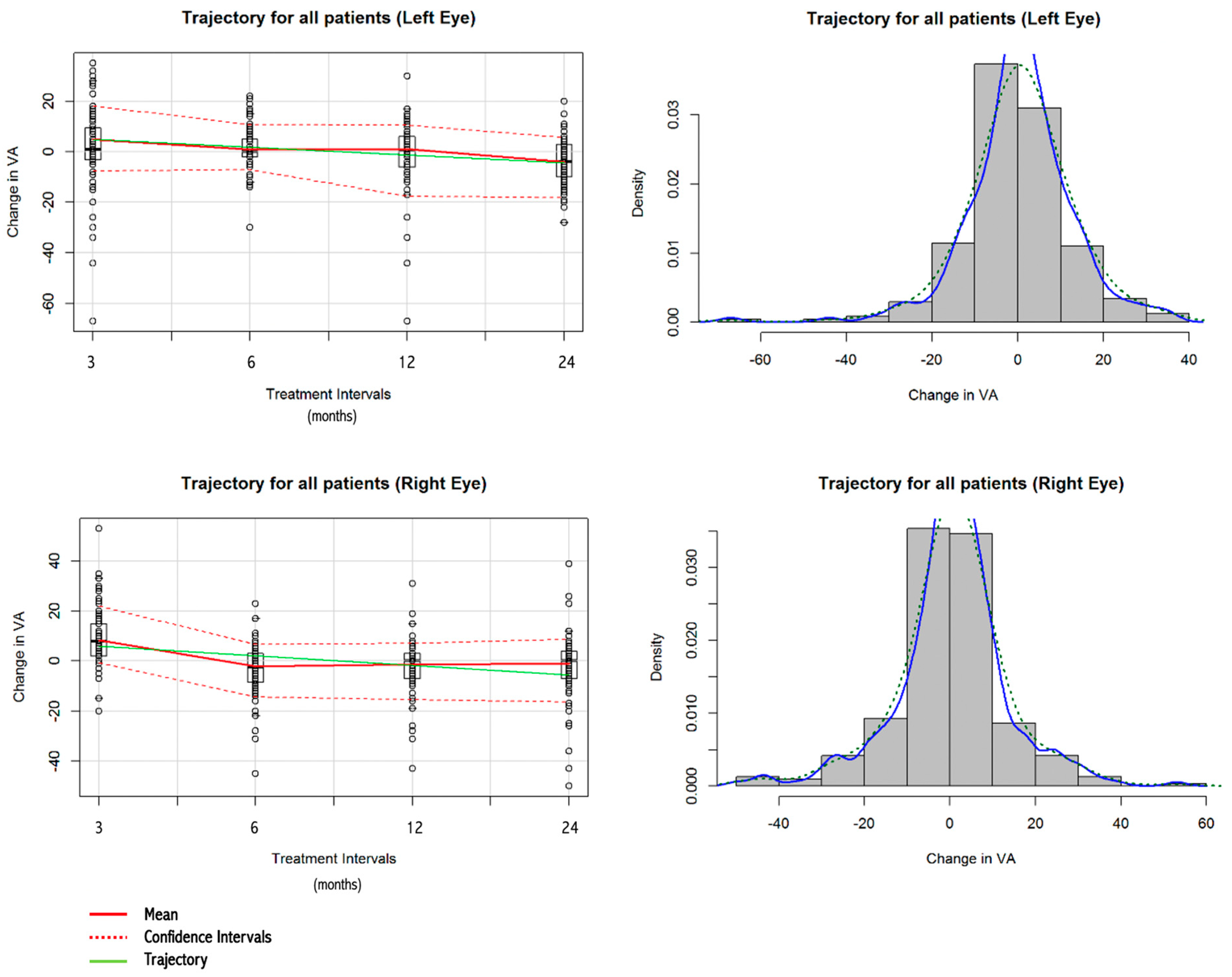
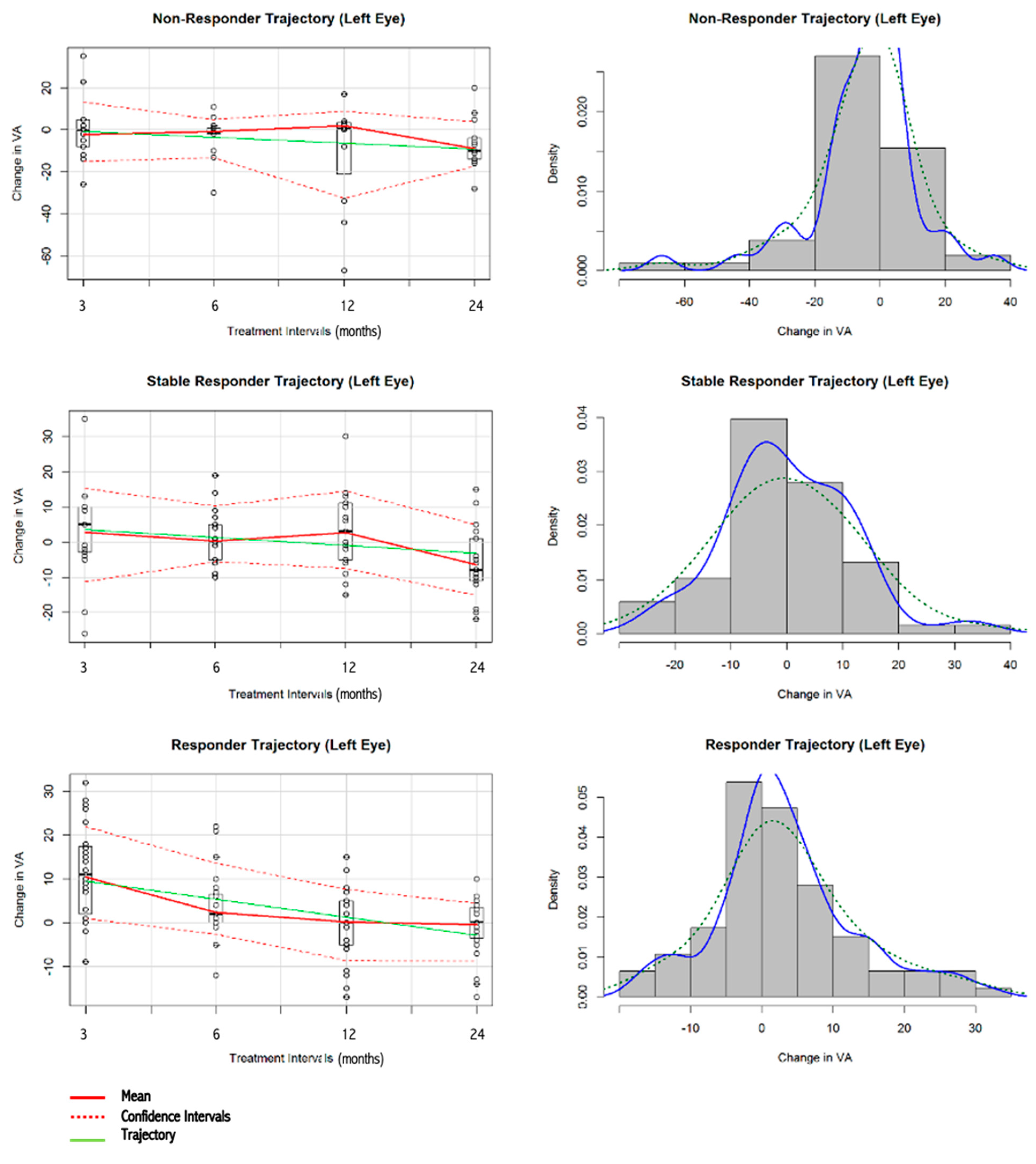
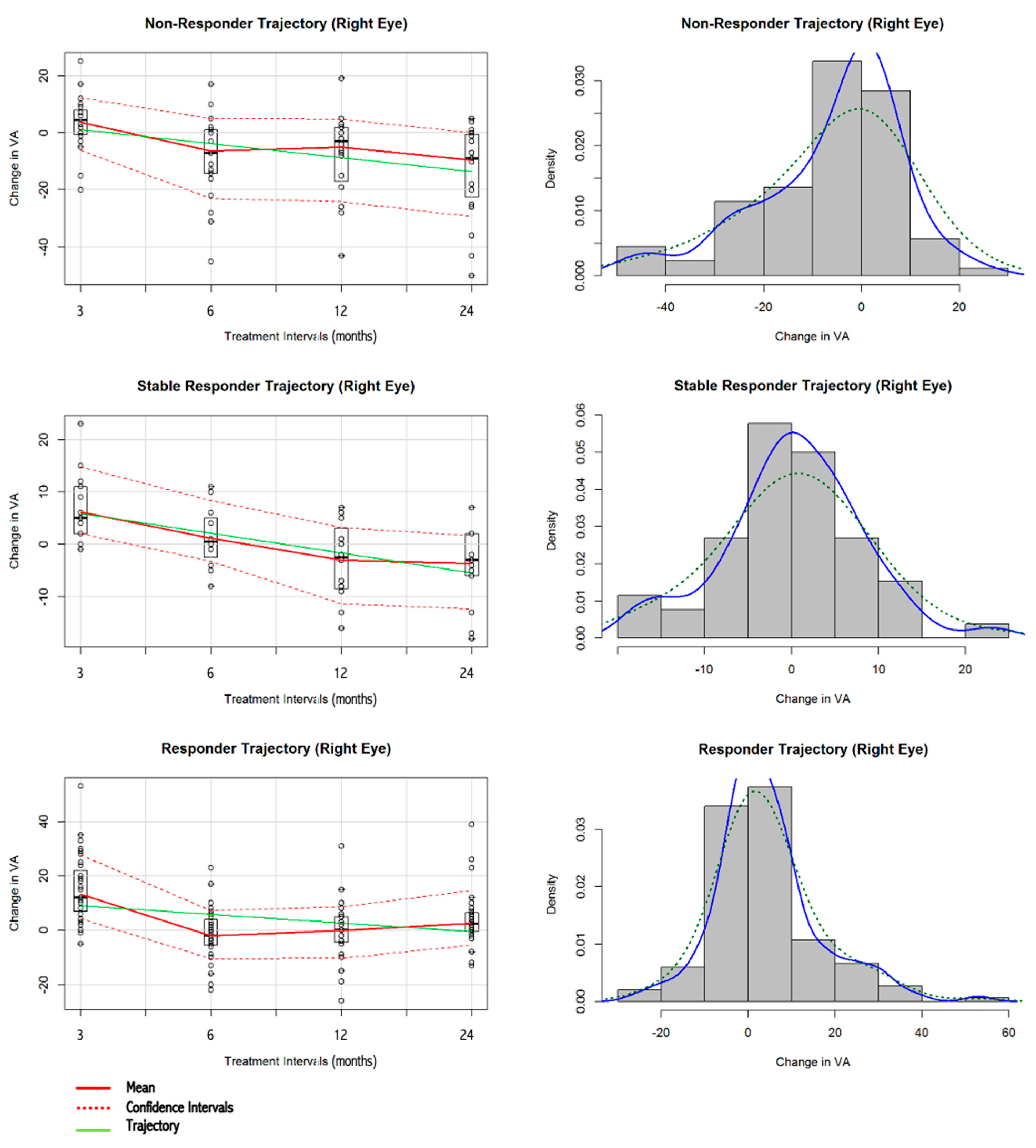
3.2. Visualisation and Skewness Statistics of VA Data

The distribution of VA changes was first visualised in the form of box plots, scatterplots, trajectory curves, and histograms. The box plots, scatterplots, and curves were superimposed. The response was reviewed as a total change in VA between each appointment/treatment interval. For example, a VA at time $t_i$ would be subtracted from the VA at $t_{i-1}$ and that would represent a change in VA between two time points.

Visualisation of the VA scores showed a normal trend when the entire cohort was viewed collectively (Figure 2). For clarity, the data were divided into groups of responders, stable responders, and non-responders. Stable responders displayed a relatively normal distribution. Interestingly, non-responders demonstrated a negative skew (Figure 3 and Figure 4). We observed a general decline in vision across all subgroups. The optimal treatment response was found at the three-month mark.

To augment the visualisation techniques, we analysed the skewness statistics (a measure of distribution asymmetry) for the LE (

Table 2. Skewness, kurtosis, and descriptive statistics for the left eye using differences between each treatment interval.

	Responders	Non-Responders	Stable Responders	All
Fisher–Pearson Skewness	0.5391	−1.1474	0.3215	−0.7333
z-value	2.1534	−3.2047	1.1576	−4.29
p-value	3.13 10−2	1.35 10−3	0.247	0.00001787
Kurtosis	3.603363	6.589836	3.637867	7.257142
Mean	3.419355	−4.711538	0.2058824	0.4533898
Standard Error	1.017073	2.252924	1.381484	0.8023191
Median	2	−1	−1	0
Standard Deviation	9.808296	16.24607	11.39201	12.32546
Sample Variance	96.20266	263.9348	129.7779	151.917
Minimum	−17	−67	−26	−67
Maximum	32	35	35	35
Sum	318	−245	14	107
Count	96	56	68	256

) and RE (

Table 3. Skewness, kurtosis, and descriptive statistics for the right eye using differences between each treatment interval.

	Responders	Non-Responders	Stable Responders	All
Fisher–Pearson Skewness	0.8378	−0.8684	−0.0251	−0.2567
z-value	3.8919	−3.1761	−0.082	−1.8709
p-value	9.95 10−5	1.49 10−3	0.9346	0.06136
Kurtosis	4.738163	3.596595	3.535297	5.483278
Mean	4.413333	−6.056818	0.2307692	0.452229
Standard Error	0.9851782	1.583727	1.115372	0.734788
Median	2.5	−1	0	0
Standard Deviation	12.06592	14.85668	8.043059	13.02048
Sample Variance	145.5864	220.7209	64.6908	169.5329
Minimum	−26	−50	−18	−50
Maximum	53	25	23	53
Sum	662	−533	12	142
Count	156	96	56	344

). As per our approach in visualisation, we first reviewed the entire patient data collectively, then we divided the patients into their respective response groups. When the patients were reviewed collectively, we noted a negative value (although not as significant as that found in non-responders). This may be a reflection of the general nature of response to anti-VEGF treatments, irrespective of response classification.

Data in Table 2 and Table 3 show that even when the skewness measure $g_1$ of the distributions is fairly moderate, there is a very significant difference in the measures of central tendency as represented by the mean and median values. Comparisons between the three groups on the basis of mean values are very different than comparisons based on median values.

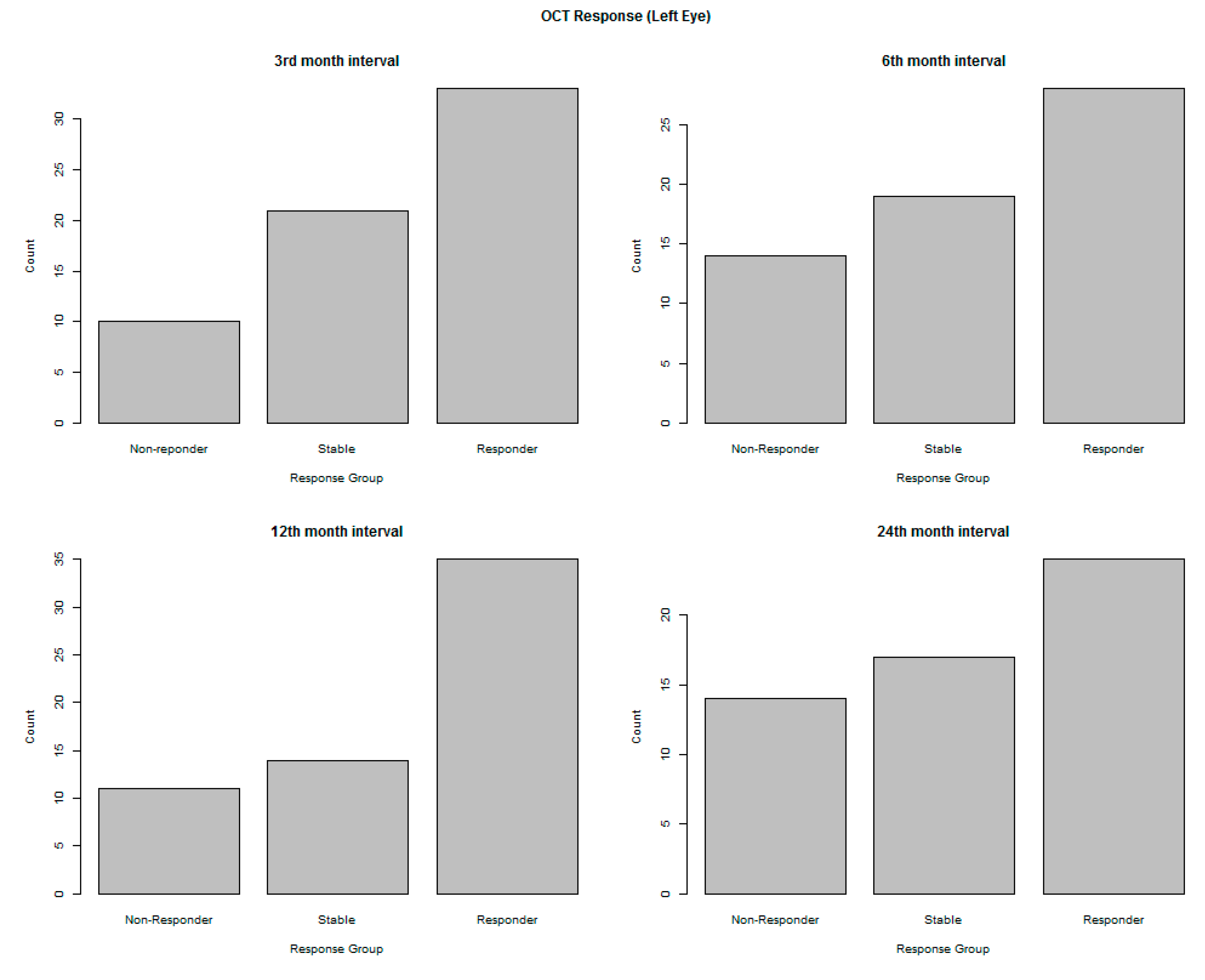
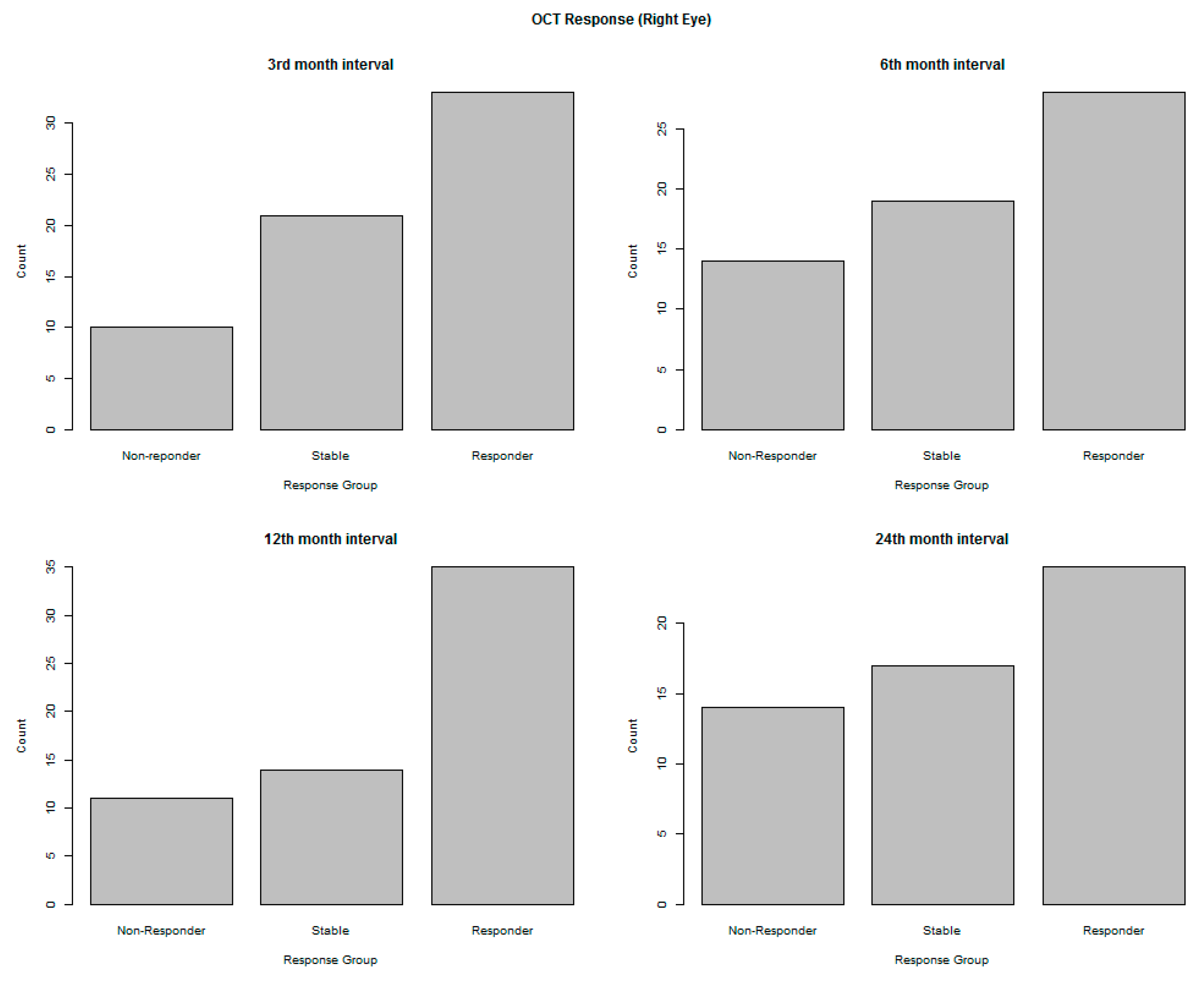
3.3. Visualisation and Summary of OCT Data

While central tendency, skewness, and kurtosis can be visualised for quantitative VA scores, the same could not be performed for OCT data as they were categorical. Instead, we opted to analyse OCT data using bar plots. Bar plots for OCT data for both the LE (Figure 5) and RE (Figure 6) show the frequency of responders, stable responders, and non-responders over a 24-month timeframe.

By the end of the 24-month treatment interval, the quantity of responders decreased and non-responders increased when compared to the baseline frequencies. The 12-month treatment stage appears to mirror the treatment group frequencies at 3 months. These outcomes suggest that vision deterioration occurs for all patients over time in this dataset, irrespective of their ability to respond to treatment.

4. Discussion

There is a continuing need to identify genetic and environmental factors affecting treatment responses to anti-VEGF injections. Apart from drug–gene interactions, environmental factors include old age, baseline VA, and the time between disease onset and treatment initiation. New information provided by medical trials would support the development of more personalised treatments for better patient outcomes and improved care and disease management.

Medical trials comparing treatment and control groups are often conducted to support research but require careful statistical analysis. In a medical trial, the clustering of treatment responses at the top or bottom of the measurement scale is referred to as a ceiling effect or floor effect, respectively. This occurs when the dose is too large (the ceiling effect) or too small (the floor effect). Possible consequences include difficulties in separating patient responses and correlating them with predictors.

In a medical study, a ceiling or floor effect may appear in the treatment group as measured by the degree of skewness in the statistical distribution of responses. The problems in the interpretation of results for highly skewed distributions can be summarised as follows:

• There is great difficulty in ranking patients in order of treatment effect, as the patient responses are the same or tightly clustered.
• If most patients have the same response, there is difficulty in correlation with potential patient-related predictors, such as age, obesity, or smoking status.
• If the statistical distribution is very skewed along the measurement scale, the arithmetic mean (as a measure of central tendency) and the variance of the patient responses are no longer representative of the group. A parametric confidence interval may even have a negative bound because the symmetrical normal distribution was assumed, rather than a skewed distribution.
• There are errors introduced in the application of standard parametric statistical tests of significance, as well as hypothesis tests, such as the comparison between the arithmetic means (treatment group vs. control group).
• It is difficult, if not impossible, to reliably fit prediction models, including machine learning algorithms.

Ceiling and floor effects may explain in part why some published experiments show contradictory results and conclusions.

Past approaches for addressing ceiling and floor effects included ignoring the effect entirely and truncation of the distributions, which leads to bias in comparing the means of two populations. Liu and Wang [31] have reviewed past attempts to ameliorate the impact of ceiling and floor effects on results and suggested an approach to help improve the accuracy in the case of the t-test and ANOVA. Šimkovic and Träuble [32] investigated a large range of statistical methods for their robustness in the presence of ceiling and floor effects using simulated datasets. They evaluated the performance of Welch’s t-test, the F-test, Mann–Whitney test, Kruskal–Wallis test, Scheirer–Ray–Hare test, and others on the estimation of group differences and confidence intervals. They advised against using the t-test and F-test in the presence of ceiling and floor effects.

In the current study, we have suggested approaches for analysing the problematic data. The results of this study and our analytic suggestions can be translated to other disciplines where continuous distributions are analysed.

The issue can be addressed at the experimental design stage by establishing a dose–response curve in a pilot study. If ceiling and floor effects are present, the dose can be adjusted to produce a more graded response between the toe and shoulder of the dose–response curve, prior to the main trial. Thus, characterizing ceiling and floor effects in dose–response models, particularly as applied in anti-VEGF response, can assist in more defined and precise treatment stratification.

If a skewed distribution is identified after data collection and treatment, there are various methods available to process the data, such as logarithmic transformation to produce a normal distribution or comparing two distributions with non-parametric tests, such as the Mann–Whitney or the Wilcoxon rank sum test. But the non-parametric tests are less sensitive and produce wider confidence intervals. The ceiling and floor effects can help inform the appropriate modifications required in the analysis of anti-VEGF data. For example, if the data present strong positive skewness, traditional logarithmic transformations may need to be coupled with a constant to ensure adequate data transformation. Thus, the techniques presented in this publication can assist in understanding and appropriately treating anti-VEGF-related data in future studies.

In the case study reported here, the Fisher–Pearson skewness metric was used to measure the degree of clustering at the high and low end of the measurement scale. The metric revealed that even moderate degrees of skewness can result in very different values for the mean vs. median values in the response and non-response groups. For example, Table 2 and Table 3 show that even moderate levels of skewness can result in divergence between the mean and median values in both the response and non-response groups by factors of two-fold to four-fold. In this case, standard parametric statistical tests based on arithmetic means cannot be used to compare the test and control groups.

When there is a significantly skewed distribution, the parametric confidence interval (CI) should be replaced by an uncertainty interval derived from the cumulative distribution function (CDF). In this case, the lower and upper bounds of the uncertainty interval can be determined from percentiles of the CDF [33]. For example, for a level of significance α = 10%, the non-parametric two-tailed 90% CI relates to the function values at the 5th and 95th percentiles of the cumulative distribution. More importantly, this uncertainty interval width in the CDF is not dependent on the shape of the statistical distribution of the data. The width of the interval between the lower and upper percentiles (e.g., 5th and 95th percentiles) from the CDF is sometimes referred to as the non-parametric confidence interval and is also used in Bayesian statistical analysis [33].

For a highly skewed distribution, the arithmetic mean should be replaced by the median (50th percentile) as an estimate of central tendency for the distribution [33]. The width of the cumulative probability distribution is a more robust representation of uncertainty because the non-parametric CI is not sensitive to outliers, contains range information, and provides stratification over the full range.

5. Conclusions

The problem of an appropriate dose can occur with a single patient or for a group of patients in a medical trial. Ceiling and floor effects relate to the clustering of patient responses around a particular level at either end of the measurement scale resulting in a skewed distribution of responses. These ceiling and floor effects may be due to a treatment dose that is either too large or too small. Exploratory data analysis and statistical moments were used to illustrate and evaluate ceiling and floor effects and their potential impact on medical trial results in the treatment of wet AMD by anti-VEGF injections.

Statistical analysis described in this case study revealed that significant errors are possible for even moderately skewed distributions in responses when comparing treatment and control groups. In the case study, the difference between the mean and median values was different by a factor of two or more in magnitude. For significantly skewed distributions, the median (not the mean) is the preferred measure of central tendency when comparing treatment and control groups.

This study adds to our understanding of patient response limits in the analysis of medical treatments involving anti-VEGF injections for wet AMD. The possible impact of skewness on study results and statistical inference was discussed, including potential errors in using standard parametric tests. Advice was provided for statistical data pre-processing and post-processing if significantly skewed distributions were present in response groups.

References

1. Chakravarthy, U.; Harding, S.P.; Rogers, C.A.; Downes, S.M.; Lotery, A.J.; Culliford, L.A.; Reeves, B.C.; IVAN study investigators. Alternative treatments to inhibit VEGF in age-related choroidal neovascularisation: 2-year findings of the IVAN randomised controlled trial. Lancet 2013, 382, 1258–1267. [Google Scholar] [CrossRef] [PubMed]
2. Bora, N.S.; Matta, B.; Lyzogubov, V.V.; Bora, P.S. Relationship between the complement system, risk factors and prediction models in age-related macular degeneration. Mol. Immunol. 2015, 63, 176–183. [Google Scholar] [CrossRef] [PubMed]
3. Buck, D.A.; Dawkins, R.; Kawasaki, R.; Sandhu, S.S.; Allen, P.J. Survey of Victorian ophthalmologists who use ranibizumab to treat age-related macular degeneration: To identify current practice and modifiable risk factors relevant to post-injection endophthalmitis. Clin. Exp. Ophthalmol. 2015, 43, 277–279. [Google Scholar] [CrossRef]
4. Wong, W.L.; Su, X.; Li, X.; Cheung, C.M.; Klein, R.; Cheng, C.Y.; Wong, T.Y. Global prevalence of age-related macular degeneration and disease burden projection for 2020 and 2040: A systematic review and meta-analysis. Lancet Glob. Health 2014, 2, e106–e116. [Google Scholar] [CrossRef] [PubMed]
5. Parmeggiani, F.; Gemmati, D.; Costagliola, C.; Sebastiani, A.; Incorvaia, C. Predictive role of C677T MTHFR polymorphism in variable efficacy of photodynamic therapy for neovascular age-related macular degeneration. Pharmacogenomics 2009, 10, 81–95. [Google Scholar] [CrossRef] [PubMed]
6. Horie-Inoue, K.; Inoue, S. Genomic aspects of age-related macular degeneration. Biochem. Biophys. Res. Commun. 2014, 452, 263–275. [Google Scholar] [CrossRef] [PubMed]
7. Coleman, H.R.; Chan, C.C.; Ferris, F.L., 3rd; Chew, E.Y. Age-related macular degeneration. Lancet 2008, 372, 1835–1845. [Google Scholar] [CrossRef]
8. Schramm, E.C.; Clark, S.J.; Triebwasser, M.P.; Raychaudhuri, S.; Seddon, J.; Atkinson, J.P. Genetic variants in the complement system predisposing to age-related macular degeneration: A review. Mol. Immunol. 2014, 61, 118–125. [Google Scholar] [CrossRef]
9. Australian Government. Department of Health and Aged Care. Section Two: The Epidemiology and Impact of Blindness and Vision Loss in Australia. Available online: http://www.health.gov.au/internet/main/publishing.nsf/ContentD1A5409787D800F2CA257C73007F12F3/$File/2.pdf (accessed on 30 September 2014).
10. Ambati, J.; Ambati, B.K.; Yoo, S.H.; Ianchulev, S.; Adamis, A.P. Age-related macular degeneration: Etiology, pathogenesis, and therapeutic strategies. Surv. Ophthalmol. 2003, 48, 257–293. [Google Scholar] [CrossRef]
11. Ratnapriya, R.; Chew, E.Y. Age-related macular degeneration-clinical review and genetics update. Clin. Genet. 2013, 84, 160–166. [Google Scholar] [CrossRef]
12. Holz, F.G.; Pauleikhoff, D.; Spaide, R.F.; Bird, A.C. (Eds.) Age-Related Macular Degeneration, 2nd ed.; Springer: Berlin/Heidelberg, Germany, 2013. [Google Scholar]
13. Francis, P.J. The influence of genetics on response to treatment with ranibizumab (Lucentis) for age-related macular degeneration: The Lucentis Genotype Study (an American Ophthalmological Society thesis). Trans. Am. Ophthalmol. Soc. 2011, 109, 115–156. [Google Scholar] [PubMed]
14. Fauser, S.; Lambrou, G.N. Genetic predictive biomarkers of anti-VEGF treatment response in patients with neovascular age-related macular degeneration. Surv. Ophthalmol. 2015, 60, 138–152. [Google Scholar] [CrossRef] [PubMed]
15. National Library of Medicine. ClinicalTrials.gov. 2015. Available online: https://clinicaltrials.gov/ (accessed on 30 October 2015).
16. Anand, A.; Sharma, K.; Chen, W.; Sharma, N.K. Using current data to define new approach in age related macular degeneration: Need to accelerate translational research. Curr. Genom. 2014, 15, 266–277. [Google Scholar] [CrossRef] [PubMed]
17. Mitchell, P. Eyes on the Future: A Clear Outlook on Age-Related Macular Degeneration; Macquaire University: Sydney, Australia, 2011. [Google Scholar]
18. Bartlett, J.D. Ophthalmic Drug Facts; Facts & Comparisons; Lippincott Williams & Wilkins: Philadelphia, PA, USA, 2013. [Google Scholar]
19. Shastry, B.S. Genetic Risk Factors in Age-Relatd Macular Degeneration. In Encyclopedia of Eye Research; Nova Science Publishers, Inc.: Hauppauge, NY, USA, 2012; pp. 1365–1376. [Google Scholar]
20. Rovner, B.W.; Casten, R.J.; Hegel, M.T.; Massof, R.W.; Leiby, B.E.; Ho, A.C.; Tasman, W.S. Improving function in age-related macular degeneration: A randomized clinical trial. Ophthalmology 2013, 120, 1649–1655. [Google Scholar] [CrossRef] [PubMed]
21. Amoaku, W.M.; Chakravarthy, U.; Gale, R.; Gavin, M.; Ghanchi, F.; Gibson, J.; Harding, S.; Johnston, R.L.; Kelly, S.P.; Lotery, A.; et al. Defining response to anti-VEGF therapies in neovascular AMD. Eye 2015, 29, 721–731. [Google Scholar] [CrossRef] [PubMed]
22. McBee, M. Modeling outcomes with floor or ceiling effects: An introduction to the Tobit model. Gift. Child Q. 2010, 54, 314–320. [Google Scholar] [CrossRef]
23. Arslan, J.; Benke, K.K. Application of Machine Learning to Ranking Predictors of Anti-VEGF Response. Life 2022, 12, 1926. [Google Scholar] [CrossRef]
24. Andrade, C. The Ceiling Effect, the Floor Effect, and the Importance of Active and Placebo Control Arms in Randomized Controlled Trials of an Investigational Drug. Indian J. Psychol. Med. 2021, 43, 360–361. [Google Scholar] [CrossRef]
25. Gelman, A. Exploratory Data Analysis for Complex Models. J. Comput. Graph. Stat. 2004, 13, 755–779. [Google Scholar] [CrossRef]
26. Behrens, J.T. Principles and procedures of exploratory data analysis. Psychol. Methods 1997, 2, 131–160. [Google Scholar] [CrossRef]
27. Huang, I.C.; Frangakis, C.; Atkinson, M.J.; Willke, R.J.; Leite, W.L.; Vogel, W.B.; Wu, A.W. Addressing ceiling effects in health status measures: A comparison of techniques applied to measures for people with HIV disease. Health Serv. Res. 2008, 43, 327–339. [Google Scholar] [CrossRef]
28. Doane, D.P.; Seward, L.E. Measuring Skewness: A Forgotten Statistic? J. Stat. Educ. 2011, 19, 1–18. [Google Scholar] [CrossRef]
29. George, D.; Mallery, M. SPSS for Windows Step by Step: A Simple Guide and Reference, 17.0 Update, 10th ed.; Pearson: Boston, MA, USA, 2010. [Google Scholar]
30. Hair, J.; Black, W.C.; Babin, B.J.; Anderson, R.E. Multivariate Data Analysis, 7th ed.; Pearson Educational International: Upper Saddle River, NJ, USA, 2010. [Google Scholar]
31. Liu, Q.; Wang, L. t-Test and ANOVA for data with ceiling and/or floor effects. Behav. Res. Methods 2021, 53, 264–277. [Google Scholar] [CrossRef]
32. Šimkovic, M.; Träuble, B. Robustness of statistical methods when measure is affected by ceiling and/or floor effect. PLoS ONE 2019, 14, e0220889. [Google Scholar] [CrossRef]
33. Benke, K.K.; Norng, S.; Robinson, N.J.; Benke, L.R.; Peterson, T.J. Error propagation in computer models: Analytic approaches, advantages, disadvantages and constraints. Stoch. Environ. Res. Risk Assess. 2018, 32, 2971–2985. [Google Scholar] [CrossRef]
Figure 1. Graphical representation of skewness. (a) Negatively skewed (i.e., left): the ceiling effect. (b) Normal distribution (centred): no effect. (c) Positively skewed (i.e., right): floor effect.
Applbiosci 02 00042 g001
Figure 2. Distribution and trajectory plots to determine ceiling effects for all patients. The box plot with a curvature (left) demonstrates the trajectory of response for all patients collectively. There is a negative linear correlation. This suggests that, irrespective of response classification, all patients have a gradual decline in vision over time. The histogram (right) appears to be relatively normal overall, although closer inspection may suggest a very slight negative skew. A normal distribution would indicate no ceiling effect. The red line represents the mean (with confidence intervals), while the green line represents the trajectory. Blue lines illustrate the distribution.
Applbiosci 02 00042 g002
Figure 3. Distribution and trajectory plots to determine ceiling effect for individual groups for left eye. The left-hand side consists of combination box plots with curvatures. These plots (irrespective of group) show that all patients have a gradual decrease in VA. This would indicate that, although some patients have a better response than others, vision deterioration was ongoing (for this dataset). The distribution on the right-hand side shows normality for responders and stable responders and a moderate negative level of skewness for non-responders. The red line represents the mean (with confidence intervals), while the green line represents the trajectory. Blue lines illustrate the distribution.
Applbiosci 02 00042 g003
Figure 4. Distribution and trajectory plots to determine ceiling effect for individual groups for right eye. The left-hand side consists of combination box plots with curvatures. These plots (irrespective of group) showed that all patients had a gradual decrease in VA. This would indicate that, although some patients have a better response than others, vision deterioration was ongoing (for this dataset). The distributions on the right-hand side show normality for stable responders, a moderate level of positive skewness for responders, and a moderate level of negative skewness for non-responders. The red line represents the mean (with confidence intervals), while the green line represents the trajectory. Blue lines illustrate the distribution.
Applbiosci 02 00042 g004
Figure 5. Bar plots for OCT data for the left eye. Patients were grouped as responders, non-responders, or stable, based on the clinical observations of retinal specialists. We note that some patients who were classified as a responder at 3 months of treatment became non-responders by the end of the 24 months.
Applbiosci 02 00042 g005
Figure 6. Bar plots for OCT data for the right eye. Patients were grouped as responders, non-responders, or stable, based on the clinical observations of retinal specialists. As with the left eye, some patients who were classified as a responder at 3 months of treatment became non-responders by the end of the 24 months.
Applbiosci 02 00042 g006