SAT-Based Synthesis and DEVS Simulation from Partial Generative Specifications for Verifiable AI

Abstract

System models and artifacts continuously require validation and refinement to address imprecise specifications and early-stage requirements in order to derive executable simulations. We propose a multi-layer approach for the automated formalization and execution of partial generative specifications derived from high-level descriptions. The first layer processes model seeds—potentially produced by large language models—that capture coarse structural information such as node relations, ordering, and timing estimates. Rather than requiring fully specified executable models from generative sources, we restrict their role to producing partial specifications, which are then completed through formal synthesis. We implement a synthesis engine based on Boolean satisfiability that constructs executable control flow structures from these partial specifications while enforcing structural consistency and execution semantics. Satisfiability modulo theories are further used to verify temporal properties and establish simulation baselines. The resulting models are then transformed into a set-theoretic discrete event system specification, enabling executable simulation via generated code artifacts. This pipeline establishes a unified pathway from partial generative artifacts to formally validated and executable models. It enables reliable and interpretable exploration of design alternatives and experimentation under formally grounded structural and temporal constraints, while providing a foundation for integrating generative modeling with rigorous execution semantics.

1. Introduction

Generative structures can provide significant advantages for streamlining system development and workflow orchestration. They extend the scope of design automation, enabling modelers and programmers to explore vast permutations within an accelerated pipeline. When such structures are semantically enhanced (e.g., from generative AI sources), the resulting artifacts can provide valuable insights. However, producing execution and sound simulations of such structures remains challenging. Even with the advent of generative models (e.g., code-writing assistants), the resulting implementations and proposals raise interpretability issues and lack correctness guarantees. They are also prone to context limits, training bias, semantic misalignment, and other known issues [1]. The generated code could often lack an underlying model or an internal grasp of intent. The emerging tools clearly indicate the need for a significant paradigm shift in the ways we approach programming. However, without practical, advanced methods of validation and interpretation, the usability of such results can be challenging to realize.

To observe the structural aspects of generative models, we conducted a preliminary, exemplary experiment using one of the publicly available large language models (LLMs) to demonstrate the variability in generated results with minimal instructions. We prompted a generic GPT-4o [2] to suggest domains and then generated a model or diagram for each domain. The generated list of domains included healthcare systems, e-commerce platforms, embedded systems, and many others. For example, we prompted a model that had not been personalized or fine-tuned with the following: “Generate a Bayesian graph example for a healthcare system ”. Then, we recorded the observed relevant metric of the resulting graph. We report the detailed observations of the selected metrics in

Table A1. Structural characteristics of database schemas, Bayesian networks, and decision trees.

Database Schemas
Domain	Tables	Relations	Total Att.
Healthcare System	6	6	40
E-commerce Platform	8	8	39
University Management System	6	7	28
Social Networking App	7	10	38
Banking and Finance	6	5	37
Hotel Booking System	5	4	29
Supply Chain & Inventory Management	7	7	34
Real Estate Portal	7	10	46
Learning Management System (LMS)	9	11	50
Transportation and Logistics	6	5	34
Bayesian Networks
Domain	Nodes	Edges	Discrete States
Medical Diagnosis	5	4	10
Fraud Detection	6	5	13
Weather Forecasting	4	4	8
Autonomous Vehicles	10	16	26
Gene Expression & Bioinformatics	7	7	14
Customer Churn Prediction	7	6	20
Financial Market Modeling	6	7	18
Ecological Modeling	5	5	14
Manufacturing & Quality Control	5	4	14
Decision Trees
Domain	Nodes	Leaf Nodes	Max Depth
Healthcare & Medical Diagnosis	13	6	4
Finance & Credit Scoring	13	7	4
Marketing & Customer Segmentation	11	6	4
Fraud Detection	11	6	4
Retail & Inventory Management	12	7	5
Manufacturing & Quality Control	9	5	4
Education & Student Performance	10	6	4
Energy Consumption Forecasting	13	7	4
Human Resources & Hiring	11	6	6
Cybersecurity	15	9	4

and

Table A2. Structural characteristics of activity diagrams and state machines.

Activity Diagrams
Domain	Nodes	Decisions	Forks & I/O
Healthcare Systems	11	1	0
Banking and Finance	12	1	0
E-commerce	11	0	0
Education and E-learning	13	2	0
Software Development	8	0	0
Telecommunications	11	2	0
Government and Public Services	14	3	0
Manufacturing and Supply Chain	11	2	0
Human Resources (HR)	12	2	0
Insurance	11	1	0
State Machines
Domain	States	Transitions
Embedded Systems	5	7
Networking Protocols	11	20
Game Development	6	10
Compiler Design	6	8
User Interface (UI) Design	9	16
Telecommunications	5	12
Robotics and Automation	6	13
Workflow & Business Process Management	8	9
Cybersecurity/Access Control	6	13
Control Systems & Mechatronics	5	8

in Appendix A. We recorded the total count for each feature (e.g., nodes, tables, or transitions) in the generated example. For instance, the generated database schema for a healthcare example consists of 6 tables and 6 relations. Whether it is a network, a process, or a diagram, the results in

Table 1. Standard deviation of structural features across formalisms.

Formalism	Features	Std. Dev.
Database Schema	Tables, Relations, Attributes	1.25, 2.20, 6.67
Bayesian Net	Nodes, Edges, States	1.87, 3.76, 5.07
Decision Tree	Nodes, Leaf Nodes, Max Depth	1.79, 1.25, 0.63
Activity Diagram	Nodes, Decisions	1.58, 0.94
State Machine	States, Transitions	1.83, 4.14

suggest some level of consistency in its general structural metrics. In extreme cases, such as the depth of a decision tree, the model generated almost all trees at the same depth. None of the generated activity diagrams included a fork node or input/output parameters, unless the model was explicitly instructed to do so. A relatively high variability score was achieved in generating transitions for state machine diagrams. Table 1 shows the standard deviation result in each observed metric. We also conducted the same experiment on Gemini 2.5 Flash [3] and observed similar patterns. While such consistency can be useful, some limitations remain to realize the potential of these models for generating large-scale, highly variable structures that are beneficial for exploratory design, combinatorial analysis, and the examination of exceptional cases [4].

Thus, such issues may pose a limitation when scaling these models to address complex systems, where validating their reasoning capacity may be challenging. The generation process and the resulting structures may fail to evolve sufficiently to meet increasing needs. Some solutions attempt to explicitly introduce intermediate tokens to enhance LLM performance and improve results. Some target specific technical features, such as backtracking knowledge sources. Addressing context length [5] is another approach to enabling larger windows in growing applications. It enhances the semantic enrichment in handling larger queries while still producing intact results [6]. However, aside from predetermined benchmarks, the degradation of context remains a challenging issue, especially when it must be reliably addressed across the broader context and scale of systems.

A possible way to address this limitation is through human feedback and instruction. However, previous research has demonstrated cases of unfaithfulness and misalignment when such models are precisely instructed as they attempt to over-optimize for the predetermined measure, rather than focusing on overall quality and correctness. We demonstrated some cases in generating diagram structures with parallel flows [4]. Other works have demonstrated inaccuracies in abstractive summarization when evaluated against historical facts [7]. Some researchers frame these issues as a form of hallucination attributed to a variety of contributing factors [1]. In this work, we address forms of misalignment and semantic misattribution, as the underlying model attempts to satisfy user-specific instructions while encountering domain limitations and imprecision.

In this article, we propose a neuro-symbolic approach to examine the expressive limits of generative models while benefiting from their ability to adapt to different domain semantics. We establish baselines for logic correctness using satisfiability encoding. We guide the model development process gradually, starting from a minimal yet continually growing set, and iteratively adding intermediary corrective and simulation layers. We aim to produce executable simulation artifacts that remain interpretable within a fully automated pipeline. Our approach relies on multiple layers of generic scaffolds that can be attached to the generative model to produce basic model-structure seeds. Afterward, the results undergo verification and enhancement steps to establish a sound, interpretable simulation.

Incomplete and Semi-Formal Model Specification

Incomplete and ambiguous specifications are common, especially in the early modeling and requirement stages. While their flexibility enables an expedited, bootstrapped development cycle, their ambiguity may not be handled correctly in downstream implementation tasks, leading to failures, costly delays, and round-trip engineering. These ambiguities, especially in complex control scenarios, can be subject to various interpretations with known trade-offs. Addressing them early on in the design stages, without overburdening the modeling process, can be advantageous. A well-designed simulation framework can then rigorously highlight and exhibit such trade-offs. We also note that some ambiguities may not necessarily arise from genuine nondeterminism, but from a missing structural formation and a partial specification. Therefore, our approach addresses such an issue by elevating partial structures through explicit formal synthesis and model refinement. We reserve stochasticity for later modeling and simulation stages.

Figure 1 illustrates common structural patterns that may result in semantic ambiguities in such diagrams. The multiple incoming or outgoing flows to/from the nodes in these diagrams require explicit handling logic with specific accounts for concurrency and order (i.e., fan-in and fan-out). Such handling, especially in complex, time-sensitive systems, as well as the presence of concurrency and parallelism, can be delegated to a specialized construct within the model. The rectangular opaque nodes, for example, represent a new node type for handling synchronization between states and actions across various system diagrams. The SAT-based encoding clearly specifies the logical condition in which such handling arises. The DEVS-based formalization enables executable simulation for further validation and analytical insights. It further enables adjustment and tooling support through fully customizable code stubs that are suitable for full software and system engineering activities. The result is an integrated approach that addresses current design flaws and contextual limitations in generative structures (e.g., those produced by an LLM) through an automated formal foundation. It benefits from the multi-domain semantic richness of LLMs to fill domain-knowledge gaps in universal formal modeling methods.

Figure 1 shows three cases where satisfiability (SAT) rules can be applied for the structural resolution. In case (i), where node c receives two incoming flows, a new fork node is synthesized to isolate concurrency logic from the action node c. A similar mechanism applies in case (ii) for the multiplicity in outgoing flows from node a. In case (iii), the approach extends to support the synthesis of more detailed precedence logic where b expects an output from a, and c expects outputs from both a and b. Case (iv) shows a more elaborate diagram with a cycle.

We note that while the present work focuses on flow-like diagrams, many semi-formal modeling notations share similar structural constructs such as branching, synchronization, and ordering constraints. This suggests that the proposed synthesis architecture could be applicable more broadly. However, extending the approach requires careful consideration of the differing levels of abstraction and execution semantics associated with other diagram types, such as state machines, which may imply distinct and elaborate simulations and transformations.

2. Related Work

The advent of LLMs has spurred research across various fields, including verification and simulation modeling. Methods for utilizing these models are still emerging. Previous research has extensively investigated the use of SAT and SMT (satisfiability modulo theories) in software and system development (e.g., [8,9]), some with a particular interest in and application of execution and simulation modeling methodology [10,11]. The automated generation and refinement of system models from partial specifications has attracted interest not from a generative model perspective but rather according to formal verification rules. Some works propose the automated completion and verification of control-flow models [8,12] and transition systems [9]. In domain-specific languages, a form of string transformation synthesis has been applied [13]. SAT-based encodings have also been applied to the analysis of concurrent models such as Petri nets, including reachability and coverability problems [14], as well as net synthesis from sequential observations [15]. More recently, SAT solving has also been applied to workflow construction and composition [16]. Symbolic reasoning techniques have long been used, demonstrating that large system state spaces can be analyzed by encoding system behavior into symbolic representations and solving the resulting logical constraints [17].

Our approach elevates the application of formal methods at a different layer by connecting a generative model (e.g., an LLM) to SAT-based synthesis. The resulting model graph utilizes both the generative model and verifier as sources for auto-completion. We cast the formal encoding at the semi-formal specification and meta-layers, addressing the different diagram types used by practitioners that go beyond basic state-transition systems in program formulation. Additionally, the devised engine addresses both structural and behavioral specifications within a minimum set of execution semantics, while enabling full-cycle development and production for simulation artifacts in later stages. For example, activity flow and process models encompass a variety of control constructs that require different approaches to account for validation and execution at lower levels. Recent advances in generative models (i.e., LLMs) offer promising partial-input seeds to address such accounts but fail to provide a complete specification under formal guarantees without an extensive technical scaffold. Such checks are often delegated to an external engine, aka agentic workflow design.

Temporal and causal properties have also been extensively researched under formal modeling conditions. A wide variety of properties in software and systems are addressed using SAT/SMT solvers in conjunction with formal methods, such as timed automata and temporal logic. Several works employ SMT to validate timing constraints in dependencies in dataflow and workflow models [18,19,20]. Linear temporal logic (LTL) and bounded model checking are also commonly used to verify reachability and safety in hardware design [21]. The execution of partial models with defects has been applied to incomplete state machines, enabling early simulation and validation [11]. Within the DEVS framework, several works explore verification through constrained finite-state spaces of simulation models [10,22]. Our approach enforces bounded checks at the design stage while enabling full-fledged simulation with open, unconstrained state spaces. We also add additional checks and corrections at the meta-layer for structural properties that are semantically significant. These additional checks enable the attainment of a richer set of executable simulations and leverage generative source regardless of their result quality. They enable the validation of generative structures with partial specifications.

Executable Modeling and Simulation

Using the DEVS formalism [23] provides a computational foundation for attaining executable simulations [24]. In contrast to traditional simulation techniques, we aim to use the DEVS-compliant set-theoretic foundation, combined with a minimal simulation engine, as a means to enable simulation models to evolve computationally. Such a trait is necessary in software and systems development due to the adaptive dynamics across multiple design and production layers and abstractions. The evolving dynamics in digital twins represent a case in point that demonstrates these needs. We adhere to the modular design to enforce explicit interface contracts. We use coupling features to facilitate communication among generative elements with distinct roles.

Several environments support DEVS-based simulation, including the open-source DEVS-Suite [25] and the proprietary MS4 Me [26]. Both primarily rely on the specification of atomic and coupled models with varying degrees of support for visualizations. Recent work [27] explores the use of generic coding assistance tools to write simulation code. The study in [28] surveys the literature on techniques for model execution.

In contrast, our approach automates the synthesis and generation of executable simulation artifacts from a high-level specification. SAT-based synthesis yields structural resolutions with control artifacts that can be directly mapped to a DEVS-based specification, enabling simulation across various timing configurations. The experimental framework enables the derivation of empirical insights with assurances of correctness under both deterministic and stochastic conditions. This work addresses limitations identified in previous research [4] at a higher design level by adding an additional synthesis layer. It reinforces the generated designs and establishes experimental baselines based on the synthesis results, while accounting for both structural graph-theoretic features and execution semantics. Rather than requiring generative models to produce fully specified structures, we deliberately restrict their role to generating partial specifications. This abstraction mitigates issues related to hallucination, prompt sensitivity, and lack of guarantees, while preserving useful domain-level structure.

Table 2. Overview of related work organized by research direction and methodology.

Research Direction	SAT/SMT-Based	Symbolic/Temporal Verification	Partial Models	Simulation/Execution
Interface and control-flow synthesis, program transformation	[9,13]	[8,9]
Concurrent systems and Petri-net synthesis	[14]		[15]
Workflow construction, model execution	[16,18]	[19,20]	[11]	[28]
DEVS modeling and simulation		[10,22]		[4,25,26,27]

summarizes the main attributes of previous studies and highlights their connection to the contribution of this paper.

3. Structural Resolution via SAT Encoding

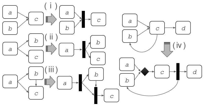
In performing SAT encoding, responsibility for constructing an executable model is shifted to a formal synthesis layer that enforces structural consistency and execution semantics. This separation enables the integration of generative flexibility with formal guarantees. First, we start by encoding constraints to resolve the cases of structural ambiguity presented in Figure 1. Once a case is identified, a control node is introduced to delegate the synchronization and merging logic. The added node represents a control construct common in flow, activity, state, process, and business process diagrams. These constructs are intended to enhance expressiveness in modeling languages and program state and flow graphs. With adequate support, such abstractions can provide a useful foundation for building simulations and accelerating the production process through advanced interpretation techniques. The problem is recognized as an ongoing challenge. Our approach in this part is to strengthen the generative process through formal synthesis and simulation techniques.

We use a generative model (e.g., an LLM) to produce a simplified structure in JSON format (or any structured file format, for that matter). Instructing the generative model to produce the final outcome may yield erroneous results or run into a context limit. It lacks the means to provide certificates, as in theorem provers, model checkers, and simulation tools. Thus, we modularize the process into an output consisting of action (atomic) nodes inferred from their pairwise precedence constraints. The produced object serves as input to the SAT program, which then introduces additional nodes. The diagram also includes initial timing estimates that we plan to use in subsequent sections for temporal verification and simulation. For example, if the generated diagram describes steps known to take a specific amount of time or to dictate an explicit time base, then the object will indicate the estimated time. During SAT-based synthesis, when a node has multiple incoming edges/flows, the program creates a new node and redirects the corresponding flow through it. In Figure 1, the diagrams are shown before and after applying the specified rules. The resulting diagrams are guaranteed to be correct, unlike possibly malformed diagrams generated by the generative source, especially for complex control dynamics that may be susceptible to misalignment.

3.1. Problem Definition

Let V denote a set of action nodes. The input specification is a precedence relation

$$P\subseteq V\times V$$

where $(u,v)\in P$ indicates that action u must precede action v.

From P, we derive predecessor and successor sets

$$pred\left(v\right)=\{u\mid (u,v)\in P\}$$

$$succ\left(u\right)=\{v\mid (u,v)\in P\}$$

Source and sink nodes are defined as

$$sources=\{v\in V\mid pred(v)=\varnothing \}$$

$$sinks=\{v\in V\mid succ(v)=\varnothing \}.$$

The objective is to synthesize an executable control-flow structure

$$G=(V^{\prime },E^{\prime })$$

that preserves the precedence constraints while assigning appropriate control semantics.

3.2. Structural Augmentation

Precedence relations alone may not encode the required control structure. To enable synthesis of forks, joins, and decision points, the solver may introduce auxiliary control nodes.

For each action $v\in V$, two optional control nodes are defined, $ctrl\_i{n}_v$ and $ctrl\_ou{t}_v.$ These represent input and output control points, respectively. The expanded node set becomes

$$V^{\prime }=V\cup \{ctrl\_i{n}_v,ctrl\_ou{t}_v\mid v\in V\}.$$

Edges in the synthesized structure may connect action nodes and control nodes.

3.3. Processing the Precedence Constraints

Given a precedence pair $(A\prec B)$, where A and B are both essential components or action nodes, we define a set of candidate paths connecting A to B based on the possible presence of synchronization. For instance, if B receives multiple incoming flows (i.e., being a destination node in multiple precedence constraints), then the path from A to B has to go through a control node with two flows (a flow from A to $sync$ and a flow from $sync$ to B), replacing the precedence constraint $(A\prec B)$ in the original diagram. Each candidate path is expressed as a Boolean formula ${\phi }_i$, involving the following edge variables representing flows and control activation flags:

• $e_{A\to B}$: Direct edge from A to B;
• $e_{A\to c{o}_A}$, $e_{c{o}_A\to B}$: Edges via the control-out (fan-out) node of A;
• $e_{A\to c{i}_B}$, $e_{c{i}_B\to B}$: Edges via the control-in (fan-in) node of B;
• $e_{c{o}_A\to c{i}_B}$: Connecting edge between control-out of A and control-in of B;
• $c{o}_A$, $c{i}_B$: Boolean flags controlling the activation of control-out and control-in.

The candidate path formulae are:

$$\begin{array}{cc}\hfill {\phi }_1:& \neg c{o}_A\wedge \neg c{i}_B\wedge e_{A\to B};\hfill \\ \hfill {\phi }_2:& c{o}_A\wedge \neg c{i}_B\wedge e_{A\to c{o}_A}\wedge e_{c{o}_A\to B};\hfill \\ \hfill {\phi }_3:& \neg c{o}_A\wedge c{i}_B\wedge e_{A\to c{i}_B}\wedge e_{c{i}_B\to B};\hfill \\ \hfill {\phi }_4:& c{o}_A\wedge c{i}_B\wedge e_{A\to c{o}_A}\wedge e_{c{o}_A\to c{i}_B}\wedge e_{c{i}_B\to B}.\hfill \end{array}$$

Let ${\mathcal{P}}_{A,B}=\{{\phi }_1,{\phi }_2,{\phi }_3,{\phi }_4\}$ denote the set of valid path encodings for the precedence $(A\prec B)$. To ensure structural consistency, we enforce the following uniqueness constraint:

$$\exists !{\phi }_i\in {\mathcal{P}}_{A,B}\mathrm{such}\mathrm{that}{\phi }_i\mathrm{is}\mathrm{true}\mathrm{where}i=1,2,3,4$$

This is implemented in the solver [29] via a pseudo-Boolean equality constraint using the following constraint:

$$\mathrm{PbEq}([{\phi }_1,{\phi }_2,{\phi }_3,{\phi }_4],1)$$

Each formula ${\phi }_i$ corresponds to one of the cases illustrated in Figure 1: ${\phi }_2$ applies to case (ii), ${\phi }_3$ to case (i), and ${\phi }_4$ to case (iii). Meanwhile, ${\phi }_1$ corresponds to the original path (the precedence pair with no added control nodes).

3.4. Control Typing

Control nodes must choose a semantic control type. Two types are supported for both input and output control: $sync$ for synchronous execution, and $select$ for exclusive choice (a relaxed control). For the input control nodes, these correspond to join and merge semantics, respectively. The output control nodes correspond to the fork, decision, and split semantics.

Let

$$type\_in\_sync\left(v\right),type\_in\_select\left(v\right)$$

denote the input control types and

$$type\_out\_sync\left(v\right),type\_out\_select\left(v\right)$$

denote the output control types.

When a control node is active, exactly one of the corresponding control types must be selected. We refer to control nodes assigned the $select$ type as relaxed controls, as they relax strict synchronization requirements by allowing a single (or a subset) incoming or outgoing flow to activate the node. In contrast, $sync$ controls enforce full synchronization across all associated flows. This distinction is used in reporting the results (e.g., “Relaxed Ctrl” in

Table 3. SAT completion results across base ambiguity cases and synthetic precedence graph families. Small, medium, and large correspond approximately to graphs with 10, 30, and 50 nodes, respectively. Relaxed Ctrl denotes the number of control nodes assigned to the select type.

Graph	Case	Nodes	Prec.	Added	Relaxed	Final	Time	Memory
			Edges	Ctrl	Ctrl	Edges	(ms)	(MB)
Base Cases	M1	3	2	1	0	3	2	17.84
	M2	3	2	1	0	3	3	18.07
	M3	3	3	2	0	5	2	18.21
	M4	4	4	2	1	6	3	18.21
	M5	10	11	3	1	14	6	18.72
DAG	Small	10	13	6	0	19	6	19.13
	Medium	30	45	24	0	69	68	39.69
	Large	50	67	25	0	92	163	71.87
Sparse Cyclic	Small	10	14	9	1	23	8	19.70
	Medium	30	47	29	2	76	86	42.33
	Large	50	70	35	3	105	207	79.40
Dense Cyclic	Small	10	28	17	0	45	5	19.92
	Medium	30	65	41	3	106	149	71.11
Random	Small	10	14	8	0	22	7	19.46
	Medium	29	45	25	0	70	59	39.23
	Large	48	70	41	0	111	491	99.67

) and in describing the synthesized structures.

3.5. Execution Semantics

To ensure that the synthesized structure admits valid execution, token propagation semantics are encoded in the model.

Let

$$token(v,t)$$

indicate that node v contains a token at step t. Transmission variables

$$send(u,v,t)$$

represent token transfer between nodes.

The execution horizon is defined as

$$H=\left|V\right|.$$

Source nodes initially hold tokens as follows:

$$token(v,0)=\left\{\begin{array}{cc}true\hfill & v\in sources\hfill \\ false\hfill & otherwise.\hfill \end{array}\right.$$

Tokens may propagate along realized precedence relations subject to control semantics.

3.6. Control Semantics and Progression

Flow activation obeys the semantics of the control types. If an output control node is typed as synchronous, flows propagate to all active successors. If an output control node is typed as $select$, at most one of its flows gets activated. If an input control node is synchronous, all incoming flows must be present before propagation. If an input control node is $select$, any incoming flow may enable propagation. These rules enforce correct execution semantics for the synthesized structure.

To prevent the synthesis of dead structures, the solver enforces that at least one sink node becomes reachable within the execution horizon:

$$\exists s\in sinks:token(s,H).$$

Source nodes initially hold tokens, and at least one sink node becomes reachable within the execution horizon. The framework supports a variety of execution specifications, including constraints on the number and distribution of tokens at sources or sinks. For the purposes of this study, we adopt the least restrictive configuration that guarantees execution progression while avoiding additional constraints that could bias the structural synthesis process.

3.7. Optimization Objective

Among the feasible solutions, the solver minimizes the number of $select$ constructs. Let

$$C=\sum _{v\in V}(type\_in\_select\left(v\right)+type\_out\_select\left(v\right)).$$

Minimizing this objective favors synchronization constructs when possible, thereby preventing degeneracy and causal collapse.

A satisfiable assignment defines the active structural edges, the inserted control nodes, the assigned control types, and the flow progression traces. Together, these define an executable control-flow graph consistent with the original precedence specification, hence the final diagram. Algorithm 1 shows the overall SAT procedure. Table 3 shows the completion results for a range of model examples. The examples include the four base cases in Figure 1, referred to as M1, M2, M3, and M4. In addition, other examples of increasing size are created to demonstrate scalability and validate the results. M5 corresponds to a wafer fabrication flow with eight nodes and eight edges [4]. Other models are generated synthetically, with the number of nodes and edges indicated in the table. Figure 1 shows the cases M1, M2, M3, and M4 of models before and after synthesis.

An input model can be obtained by calling the LLM API (i.e., GPT-4o), which returns a JSON structure containing a list of nodes and precedence constraints. An example is shown in Listing 1.

Listing 1. Sample model seed in JSON response.

Algorithm 1 SAT-Based Typed Structural Resolution from Precedence Constraints
	Input: A set of action nodes V and precedence relations $P\subseteq V\times V$
	Output: A synthesized executable control-flow structure with typed control nodes
1:	Compute predecessor and successor sets for all $v\in V$
2:	Derive source nodes, sink nodes, and horizon $H\leftarrow \left|V\right|$
3:	for each action $v\in V$ do
4:	Create optional control flags $\mathtt{ctrl}\_\mathtt{in}\left[v\right]$ and $\mathtt{ctrl}\_\mathtt{out}\left[v\right]$
5:	Activate $\mathtt{ctrl}\_\mathtt{in}\left[v\right]$ iff ${\mathrm{deg}}^{-}\left(v\right)>1$ and $\mathtt{ctrl}\_\mathtt{out}\left[v\right]$ iff ${\mathrm{deg}}^{+}\left(v\right)>1$
6:	Create typing variables:
$\mathit{type}\_\mathit{in}\_\mathit{sync}\left[v\right],\mathit{type}\_\mathit{in}\_\mathit{select}\left[v\right],\mathit{type}\_\mathit{out}\_\mathit{sync}\left[v\right],\mathit{type}\_\mathit{out}\_\mathit{select}\left[v\right]$
7:	Enforce exclusive typing for each active control node
8:	end for
9:	Create Boolean edge variables for all candidate edges
10:	for each precedence pair $(A,B)$ do
11:	Let $c{o}_A\leftarrow \mathtt{ctrl}\_\mathtt{out}\left[A\right]$, $c{i}_B\leftarrow \mathtt{ctrl}\_\mathtt{in}\left[B\right]$
12:	Define path options:
$\begin{array}{l}{\phi }_1\leftarrow \neg c{o}_A\wedge \neg c{i}_B\wedge e_{A\to B}\\ {\phi }_2\leftarrow c{o}_A\wedge \neg c{i}_B\wedge e_{A\to c{o}_A}\wedge e_{c{o}_A\to B}\\ {\phi }_3\leftarrow \neg c{o}_A\wedge c{i}_B\wedge e_{A\to c{i}_B}\wedge e_{c{i}_B\to B}\\ {\phi }_4\leftarrow c{o}_A\wedge c{i}_B\wedge e_{A\to c{o}_A}\wedge e_{c{o}_A\to c{i}_B}\wedge e_{c{i}_B\to B}\end{array}$
13:	$\mathtt{PbEq}([{\phi }_1,{\phi }_2,{\phi }_3,{\phi }_4],1)$
14:	Define $\mathtt{relation}[u,v]$ to indicate that precedence $(u,v)$ is structurally realized
15:	end for
16:	Create token variables $\mathtt{token}[v,t]$ for all $v\in V$ and $0\le t\le H$
17:	Create transmission variables $\mathtt{send}[u,v,t]$ for all $(u,v)\in P$ and $1\le t\le H$
18:	Initialize tokens at source nodes
19:	for $t=1$ to H do
20:	Constrain token transmission along structurally realized precedence relations
21:	Enforce input/output semantics:
	$sync$ input/output requires from/sends to all active predecessors/successors $select$ input/output accepts/sends from/to one active predecessor/successor
22:	Update token persistence and propagation at each node
23:	end for
24:	Enforce reachability of at least one sink node by time H
25:	Minimize the total number of select-type control assignments
26:	Run the SAT/SMT optimization solver
27:	if sat then
28:	Extract active edges, activated control nodes, assigned control types, relaxed (select-type) control nodes, and token traces
29:	end if

In this example (Listing 1), node A has precedence over both B and C, and represents the structural characteristic shown in case (ii) of Figure 1. Such sync-out (multiple outgoing flows) or sync-in (multiple incoming flows) configurations trigger the insertion of a $sync$ node to handle synchronization semantics. The associated numbers with each precedence represent transition durations that we will use in the temporal validation and simulation stages in Section 4 and Section 5.

The SAT formulation solves small and medium instances in milliseconds and scales to graphs with up to 50 nodes and 70–90 precedence constraints, achieving sub-second times. Cyclic graphs require additional control insertion, resulting in larger synthesized structures and greater solver effort. Dense cyclic graphs are the most challenging due to increased semantic propagation requirements. An ablation experiment (

Table 4. Effect of execution horizon on dense cyclic graphs.

Nodes	Prec.	Added	Relaxed	Final	Time (ms)
50	94	63	6	157	552

) shows that reducing the execution horizon substantially decreases solve time, indicating that the temporal token propagation layer dominates the computational cost.

The graph families used in the evaluation are synthetically generated in order to provide controlled variations in size and structural characteristics. These benchmarks allow us to systematically assess the performance of the SAT-based synthesis procedure under different conditions. In practice, however, this approach is intended to operate on models produced by generative modeling workflows, where precedence structures arise as artifacts of automated or semi-automated model construction.

The following are descriptions of the columns in Table 3:

• Nodes: The number of nodes in the original model.
• Prec. Edges: The number of defined precedence constraints between nodes.
• Added Ctrl: The number of control nodes inserted by the solver to enforce unambiguous control flow.
• Relaxed Ctrl: The number of control nodes for which the solver must assign the $select$ type (i.e., non-synchronizing control semantics) to ensure a feasible progression.
• Final Edges: The total number of edges in the completed model after adding control nodes.
• Time (ms): The time taken by the Z3 solver to solve the encoding, measured in milliseconds.
• Memory (MB): The peak memory usage recorded during the solving process.

These metrics collectively characterize the solver’s performance and the structural complexity of the model as it grows in size. The performance demonstrates the potential applicability and feasibility of this approach in real-time inference. A snippet of the implementation code is shown in Listing 2.

Listing 2. Code snippet for the SAT-based synthesis, written in Python 3.12.12 using Z3.

An important advantage of the SAT-based formulation is that multiple synthesis objectives are handled within a unified framework. Specifically, the solver simultaneously performs structural synthesis of edges, semantic validation via propagation constraints, and optimization of control semantics by minimizing the number of select-type constructs. This integration allows the solver to search directly over executable control-flow structures while guaranteeing consistency with the precedence specification.

3.8. Complexity Discussion

Since SAT solving is NP-complete in general, the worst-case complexity of the synthesis procedure is exponential in the number of Boolean variables.

Let $\left|V\right|$ denote the number of nodes and $\left|P\right|$ the number of precedence relations. The formulation introduces Boolean variables for control activation, control typing, structural edges, precedence realizations, and token propagation. Control flags and typing variables contribute $O\left(\right|V\left|\right)$ variables. Each precedence relation introduces a constant number of candidate structural edges, yielding $O\left(\right|P\left|\right)$ edge variables. The execution semantics introduce token variables $token(v,t)$ for all nodes and time steps $0\le t\le \left|V\right|$, resulting in $O\left(\right|V{|}^2)$ variables. Additionally, token transmission variables $send(u,v,t)$ are created for each precedence relation and time step, resulting in $O\left(\right|P\left|\right|V\left|\right)$ variables. Consequently, the total number of Boolean variables in the encoding grows as $O\left(\right|P\left|\right|V|+|V{|}^2)$.

Although the worst-case complexity is exponential, modern SAT/SMT solvers can efficiently handle instances of practical size for this study due to sophisticated optimizations. Also, the choice of the horizon is conservative. Reducing it to a more effective heuristic could further reduce complexity, as confirmed by the ablation case (Table 4). In practice, the limited scalability due to the bounded execution encoding can be mitigated by modular construction within the DEVS framework. Structural completion can be applied to smaller subsystems, which are then composed hierarchically within a DEVS model. This approach enables exact synthesis at the component level while relying on DEVS-based simulation and validation to evaluate the behavior of larger systems and yet unforeseen emergent properties. Consequently, SAT-based completion and DEVS-based modeling form complementary layers. The former ensures structural correctness of the control patterns given the execution semantics of the latter, while the latter supports scalable composition and experimentation.

4. Temporal and State Formalization Using SMT and DEVS

At this stage, we draw on DEVS semantics to infer the state properties. In DEVS formalism, each atomic model evolves over a continuous time base and is formally defined by:

• Input/output event sets X and Y;
• A state set S including passive and active;
• A time advance function $ta:S\to {\mathbb{R}}_{\ge 0}\cup \{\infty \}$;
• A transition function $\delta :S\times (X\cup \{\varnothing \left\}\right)\to S$ (${\delta }_{internal},{\delta }_{external},{\delta }_{confluent}$);
• An output function $\lambda$.

We formalize the resulting structures from the resolution stage in Section 3 with a set of atomic models. The goal is to predefine formal modeling templates and then parametrize them using verified model results. For action and $sync$ nodes, we specify two atomic models, one for each type. The atomic model for actions begins in the passive state with $ta=\infty$, and upon receiving input, it transitions to active for a fixed duration $t_n$ before returning to passive. The atomic model for $sync$ nodes consists of three phases: passive, waiting, and enabled. A $sync$ node becomes enabled only after receiving inputs from all its incoming flows. Once each model is instantiated, the coupled model forms the entire structure of atomic models, with couplings corresponding to the edges connecting them.

A variety of state and temporal validations can take place using SMT. The validations are centered around durations that symbolically correspond to a node’s active processing of some input. The finish time can be characterized as the sum of the start time and duration, and so on.

Thus, each node n is associated with the following: start time $s_n$, defined by the arrival of the input from the predecessor node; duration $t_n$, defined by the initial time estimate; and finish time, $f_n=s_n+t_n$. The system is initialized with $s_n,f_n=\infty$ for all nodes. In the case of single-input processing (only a single input can be present in the system) and an acyclic diagram, SMT constraints can be used to ensure the following:

Causal Start Constraint:

$$s_n\ge \underset{p\in \mathrm{preds}\left(n\right)}{\max }{f}_p$$

Guarantees that a node starts only after all its predecessors have completed.

$Sync$ Activation:

$$s_{sync}<\infty \iff \forall p\in \mathtt{preds}\left(sync\right),f_p<\infty$$

Ensures $sync$ nodes activate only when all required inputs are present.

Sequential Execution Consistency: We identify all edge pairs in the resulting diagram $(p,q)$ such that $p\prec q$, and enforce

$$f_p\le s_q\vee f_q\le s_p$$

The constraint prohibits causally ordered nodes from being in active states simultaneously, ensuring that either node must finish before the other starts.

Deadline Bound: Let $T_{\mathtt{total}}={\max }_{n\in \mathtt{terminal}\mathtt{nodes}}{f}_n$ represent the total completion time. This bound is inferred automatically by computing the longest edge path in a cycle-free diagram as follows:

$$T_{\mathtt{total}}\le \sum _{n\in \mathtt{critical}\mathtt{path}}{t}_n$$

Bottleneck Identification: The bottleneck edge is the edge with the longest duration among all edges on the critical path. We extract the length of such a path post-solution by comparing the durations of all edges.

We associate duration with the edges to allow nodes with multiple outgoing flows to have different transition times depending on the edge source and destination.

Table 5. SMT-based temporal and state validation results for sample DAGs.

Metric	i	ii	iii	iv	v	vi	vii
Inferred Total Time	3	3	4	12	19	21	22
Number of Node	3	3	3	8	12	12	102
Number of Precedence	2	2	3	8	14	23	151
Bottleneck Node	2	2	2	5	6	6	4
Bottleneck Duration	2	2	2	4	4	4	4
Z3 Solver Statistics
Arith. Lower Bounds	15	15	21	77	200	309	1615
Arith. Upper Bounds	16	18	24	74	232	484	2259
Tableau Columns	25	27	37	132	375	641	3259
Tableau Rows	14	16	24	107	332	582	2872
Pivots	7	8	10	21	40	56	373
Row Summations	15	26	45	225	1093	1880	8709
Boolean Variables	31	33	45	151	432	793	3874
Clauses Created	3	6	13	66	166	292	1250
Decisions	1	0	0	11	68	157	835
Resource Limit Count	1861	2111	3197	14,291	64,177	113,837	577,358
Memory Usage (MB)	17.35	17.35	17.27	17.36	17.47	17.52	18.47
Max Memory (MB)	17.65	17.65	17.66	17.87	18.51	19.28	26.72
Time	0.00	0.00	0.00	0.00	0.01	0.01	0.04

shows the results of executing the SMT-based procedure in Z3 [29]. We also present the SMT implementation in Listing 3 for the critical-path calculation. We use the results from this step to establish the deterministic baseline for the simulation experiment and adjust the input-generation pressure by calibrating the inter-arrival time to induce more or less parallelism across the model [4]. We plan to examine further configurations of path topology and connectivity degrees (e.g., strongly connected components) in future work.

Listing 3. Code snippet determining the critical path and verifying the temporal properties, written in Python using Z3.

Notes on Handling Multiple Input Traces

The formulated rules can be extended to verify systems with concurrent inputs. Causal start, $sync$ activations, and finish times will be input-sensitive and therefore checked for each input. For k parallel executions over a shared model, each constraint requires k validations to account for all input traces for each input $i=1,\dots ,k$. For example, the causality start constraint can be formulated as $s_n^{\left(i\right)}\ge {\max }_{p\in \mathtt{preds}\left(n\right)}{f}_p^{\left(i\right)}$, indicating that for each input i, each node n can only start after all precedent nodes finish processing that input.

Additional constraints can also be formulated to verify system-level properties. Since nodes may handle multiple input arrivals, constraints regarding queuing or dropping semantics can provide a critical assessment of the system, especially under pressure tests. The insights gained from these properties, in turn, can inform the generative and synthesis processes, further optimizing the model. For example, additional nodes can be added to the model if the system exceeds an average waiting time threshold. Other system-level constraints can also be added, such as a total termination time for a certain number of inputs, as well as other reachability and safety features. In this paper, we will not explicitly formulate these constraints and instead refer the reader to the established literature on this subject [30]. We focus on the prospect of automating such insights within a fully adaptive generative modeling process and on drawing on them to establish baselines for the simulation experiments. We will demonstrate some aspects of end-to-end automation in the simulation section.

5. Executable and Stochastic Simulation

In this section, we present the results of the verified modeling artifacts via an executable simulation. To conduct our experiment, we use activity and action flow semantics to specify the behavior. The flow-based and I/O communications make such a representation well suited to serve as an expressive layer of DEVS-based operational semantics.

Thus, we begin by formalizing three key elements of the activity and action flow diagram metamodel: the action, the control (also known as fork/join and decision/merge), and the entire activity diagram. The first two elements are modeled as atomic units, and their instances are coupled to represent the entire activity. We describe fork/join in $sync$ to represent synchronization, and the decision/merge nodes in the $select$ atomic model to represent conditional features in the simulation workflow. We plan to cover a wider set of control nodes in high-level engineering languages, such as SysML [31] and UML [32], as well as general orchestration flows in software and hardware deployments (e.g., Terraform [33]), among others. Recent advances in AI coding assistance tools with limited context lengths underscore the need and potential to revisit the application of disciplined methods to approach modularity and code synthesis.

We formulate the set-theoretic specification of the $sync$ nodes in a DEVS-compliant manner, thereby making them amenable to executable simulation in subsequent steps.

$$\begin{array}{cc}\hfill SYNC& =\langle X,Y,S,{\delta }_{ext},{\delta }_{int},{\delta }_{con},\lambda ,ta\rangle ,\hfill \\ \hfill X& =In\times V,In=\{i{n}_1,\dots ,i{n}_n\},\hfill \\ \hfill Y& =Out\times V,Out=\{ou{t}_1,\dots ,ou{t}_m\},\hfill \\ \hfill S& =\{\mathsf{passive},\mathsf{waiting},\mathsf{enabled}\}\times {\mathbb{R}}_{0,\infty }^{+}\times 2^X\times (In\to \mathbb{B}),\hfill \\ \hfill T^{\prime }& =T\cup \left\{\right(in,v\left)\right\},\hfill \\ \hfill C^{\prime }& =C[in\mapsto \top ],\hfill \\ \hfill {\delta }_{ext}((phase,\sigma ,T,C),e,(in,v))& =\left\{\begin{array}{cc}(\mathsf{waiting},\infty ,T^{\prime },C^{\prime }),\hfill & \exists i{n}^{\prime }\in In:C^{\prime }\left(i{n}^{\prime }\right)=\perp ,\hfill \\ (\mathsf{enabled},0,T^{\prime },C^{\prime }),\hfill & \forall i{n}^{\prime }\in In:C^{\prime }\left(i{n}^{\prime }\right)=\top ,\hfill \end{array}\right.\hfill \\ \hfill {\delta }_{int}(ph,\sigma ,T,C)& =(\mathsf{passive},\infty ,\varnothing ,C_0),C_0\left(in\right)=\perp ,\hfill \\ \hfill {\delta }_{con}(s,ta\left(s\right),x)& ={\delta }_{ext}({\delta }_{int}\left(s\right),0,x),\hfill \\ \hfill \lambda (\mathsf{enabled},\sigma ,T)& =(p,T),p\in Out,\hfill \\ \hfill ta(phase,\sigma )& =\sigma .\hfill \end{array}$$

We also formulate the specification of action nodes in a similar manner. For brevity, we present only the specification of the external transition, internal transition, and output function.

$$\begin{array}{cc}\hfill {\delta }_{ext}((phase,\sigma ,T,C),e,(in,v))& =(\mathsf{enabled},\tau (in,v),(in,v),C);\hfill \\ \hfill {\delta }_{int}(phase,\sigma ,T,C)& =(\mathsf{passive},\infty ,T,C);\hfill \\ \hfill \lambda (\mathsf{enabled},\sigma ,T,C)& =(out,v)\mathrm{where}task=(in,v).\hfill \end{array}$$

And the following includes the specifications of the external transition, internal transition, and output function of the $select$ node.

$$\begin{array}{cc}\hfill {\delta }_{ext}((phase,\sigma ,T,C),e,(in,v))& =(\mathsf{enabled},0,(in,v),C);\hfill \\ \hfill {\delta }_{int}(phase,\sigma ,T,C)& =(\mathsf{passive},\infty ,(in,v),C);\hfill \\ \hfill \lambda (\mathsf{enabled},\sigma ,T,C)& =(p_i,v)\mathrm{if}task=(in,v)\wedge \mathrm{cond}(p_i,in,v)=\mathsf{true};\hfill \\ & \mathrm{where}{p}_i=\mathrm{choose}\{p\in Out\mid \mathrm{cond}(p,in,v)=\mathsf{true}\}.\hfill \end{array}$$

Finally, the activity can be formulated with a corresponding coupled model. The set D consists of the atomic models of types action, $sync$, and $select$.

$$A=\langle X,Y,D,\{M_d\mid d\in D\},EIC,EOC,IC\rangle$$

For clarity, we provide a brief, concrete example of how C (Boolean completion map) and T (set of inputs) evolve during a simple external transition for a sync-in node with two predecessors. Consider a sync-in node with two predecessor inputs, $In=\{i{n}_1,i{n}_2\}$. Initially, the node is in the passive state

$$(\mathsf{passive},\infty ,\varnothing ,C_0),C_0\left(i{n}_1\right)=\perp ,C_0\left(i{n}_2\right)=\perp .$$

Suppose an external event $(i{n}_1,v_1)$ arrives first. Then, the external transition updates the received input set and completion map to

$$T=\left\{(i{n}_1,v_1)\right\},C\left(i{n}_1\right)=\top ,C\left(i{n}_2\right)=\perp ,$$

so the node moves to

$$(\mathsf{waiting},\infty ,\left\{(i{n}_1,v_1)\right\},C).$$

At this point, synchronization is not yet achieved because the second required input has not arrived. Next, suppose a second event $(i{n}_2,v_2)$ arrives. The state is then updated to

$$T=\{(i{n}_1,v_1),(i{n}_2,v_2)\},C\left(i{n}_1\right)=\top ,C\left(i{n}_2\right)=\top ,$$

which satisfies the synchronization condition for all required inputs. The node therefore moves to the enabled state

$$(\mathsf{enabled},0,\{(i{n}_1,v_1),(i{n}_2,v_2)\},C),$$

allowing the output function $\lambda$ to emit the synchronized token bundle. After the internal transition, the node resets to

$$(\mathsf{passive},\infty ,\varnothing ,C_0).$$

We note that in the implementation, each input port may maintain a queue of pending arrivals. Thus, if two consecutive events arrive on the same input port (e.g., $i{n}_1$) before another required predecessor input is received, both events may be buffered at the implementation level. The abstract state components T and C only record which required inputs have been observed and whether synchronization has been achieved. Accordingly, the formalization captures the logical enabling condition of the $sync$ node, while the simulator configuration allows for using per-port queues to preserve multiplicity or arrival order, in addition to other policies.

Now that we have formulated the DEVS specifications, we use Acceleo [34] to write the code templates for each node. Then, the code-generation process parametrizes these templates, providing all executable code snippets necessary to run the experiment. We generated Java code for the DEVS-Suite and MS4 Me simulators. We also implemented a DEVS simulator in JavaScript 1 that can run simulations in a web environment via model interpretation. In this experiment, we will use an MS4 Me simulator to generate the simulation results and Matplotlib 3.10.1 [35] for visualization.

Simulation Experiment

We will begin by demonstrating the approach with an illustrative example. We then present a more practical case of sensor fusion.

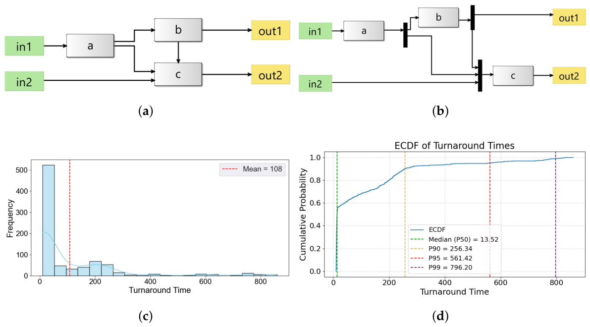
The first example diagram shown in Figure 2 consists of two input parameters, three action nodes, two output parameters, and seven flow edges to illustrate various precedence patterns. Figure 2a shows the example before the synthesis. Figure 2b shows the diagram after synthesizing the $sync$ nodes. The resulting diagram can be readily transformed into a coupled DEVS Markov model with a predefined experimental frame. The transformation is performed using Acceleo code templates to generate Java code that is executable by the MS4 Me simulator. The initial timing assignments for the action states are set to one, following an exponential distribution. The input generator alternately dispatches outputs to the coupled model: first to $i{n}_1$ and then to $i{n}_2$. The inter-arrival time is set to ten.

For illustrative purposes, we set the time for action c to 10, assuming an exponential distribution. Figure 2c,d show the obtained turnaround times after running the experiment for 10,000 time units. Both charts validate the initial timing assignments and the realization of the formal semantics during execution. The histogram shows heavily right-skewed data with two distinct regimes. The clustered times correspond to most jobs that traverse the path involving the actions a and b. The extended tail represents the turnaround times for jobs that go through c. This result is noticeable due to the empirical cumulative distribution function (ECDF). The synthesized synchronization node before c drives a skewed distribution with a median of 13.52, while 5% of cases exceed 561.

Such a combination of generative models, verifiable synthesis, and formally specified executable simulations may provide a foundation for describing and exploring behavioral dynamics within an automated modeling pipeline. For instance, the long-tail behavior observed in the turnaround-time distribution is consistent with the temporal constraints verified by the SMT layer. In particular, the action corresponding to node c has an associated processing time constraint (set to 10 units in the experiment) that participates in the SMT-based critical path validation. The stochastic simulation then samples execution paths according to the model’s structure and service-time distributions. Because the SMT validation guarantees that these precedence and timing constraints are satisfiable and causally consistent, the simulation results reflect valid executions of the formally validated model rather than artifacts introduced by the simulation environment. The resulting analytical plots, therefore, provide empirical confirmation that the observed turnaround-time behavior remains consistent with the SMT-validated temporal constraints.

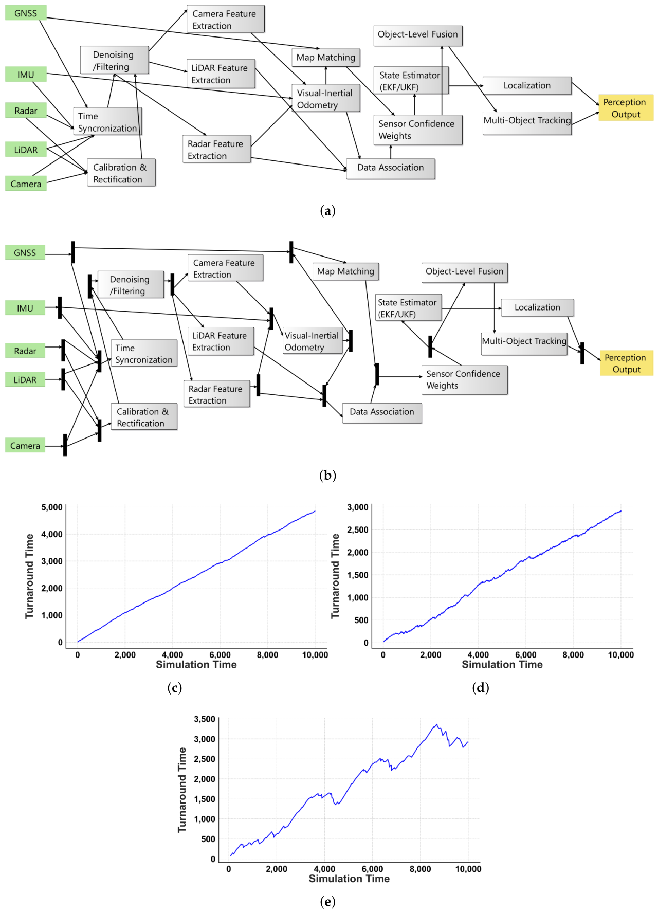
After validating the simulation results in a simple example, we demonstrate the approach’s capacity to describe domain-specific cases by using a more detailed example of a sensor fusion architecture commonly used for situational awareness in autonomous perception (Figure 3). We instructed GPT-4o to “generate a diagram for sensor fusion flow.” We implemented a tool that automatically renders the generated JSON file into an activity flow diagram. However, the devised approach aims to accommodate large structures with complex, evolving control dynamics. Figure 3a shows the generated diagram. Figure 3b shows the diagram after synthesis. As in the first example, the initial timing assignments for the action nodes are set to 1, assuming an exponential distribution. In the initial experiment, the input generator alternately dispatches outputs to the coupled model via each of the four input parameters. The inter-arrival time is set uniformly with bounds [0, 1]. Figure 3c shows the resulting turnaround times after running this experiment. Then, we adjust the inter-arrival time for the next two experiments to 1 and 10, with the turnaround time results shown in Figure 3d and Figure 3e, respectively. 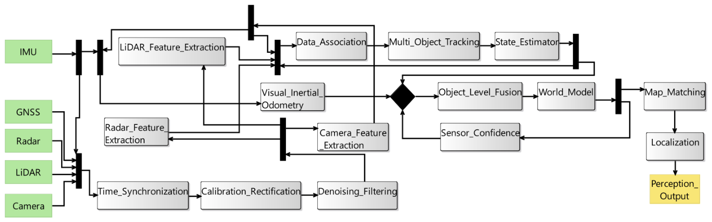Figure 4 shows another generated example for the sensor fusion pipeline with one relaxed (select-type) control node.

This example demonstrates the applicability of our proposed pipeline and its scalability in handling generated structures with behavioral and timing dynamics. The SAT-based synthesis is used to ensure that the generated structures admit a consistent executable interpretation, establishing a structurally valid progression of control flow. The resulting structures can then be transformed into parallel DEVS models while preserving their behavioral semantics. Within this setting, SAT-based reasoning provides a precise mechanism for ensuring structural consistency, whereas DEVS-based simulation enables broader exploration of system behavior through dynamic execution. This perspective aligns with earlier work emphasizing the importance of semantic-preserving transformations between formal analysis and simulation environments [36]. When the initial models are generated from AI-assisted artifacts, the process can naturally support iterative cycles in which synthesis, simulation, and validation are repeatedly applied, enabling continuous refinement of both the generated structures and the behavioral scenarios explored.

6. Conclusions

Our goal in this work is to leverage the generative capacity of recent AI models (i.e., generative models such as LLMs) to produce results with sound structures that are enriched with domain knowledge. We propose an approach to obtain the partial specifications of a timed activity and action flow diagram from a generative model in a structured format. Then, we subject the resulting structure to SAT-based synthesis to identify and rectify potential design flaws, thereby further enriching the model. Such enrichment is further compounded by its transformation into a set-theoretic DEVS-compliant specification and by code-generation templates. We demonstrate the approach using executable simulations and experiments. The obtained results and visualizations demonstrate the validity and key aspects of the automation’s consistency in the proposed pipeline. The results suggest that generative control flow structures can be synthesized with formal guarantees of correctness and executability when SAT-based structural synthesis is integrated with DEVS modeling and execution semantics. This capability is particularly valuable for complex synthesis problems that require precise and reliable execution. By embedding synthesis, validation, and simulation within a unified automated pipeline, the proposed framework provides a practical, formally grounded pathway for generating executable models.

While the proposed pipeline is motivated by structural imperfections observed in generative model outputs, these imperfections are addressed through formalization under execution semantics. Rather than requiring generative models to produce fully specified and executable flow structures—which can be unreliable due to hallucinations, instruction sensitivity, and lack of guarantees—we constrain their role to generating partial specifications. The synthesis process then constructs a complete and executable model by enforcing structural and semantic consistency. Accordingly, the current evaluation focuses on representative precedence structures capturing execution-relevant structural ambiguities, rather than directly benchmarking raw LLM-generated outputs. We acknowledge that this abstraction introduces a gap between the motivating generative artifacts and the evaluated instances, as the current experiments do not directly measure performance on raw LLM-generated structural outputs. Extending the evaluation to fully integrate end-to-end pipelines operating on unfiltered generative artifacts remains an important direction for ongoing and future work.

Despite some promising results, several limitations remain. The current synthesis procedure guarantees a weak progression property, ensuring that execution can propagate from sources to at least one sink, but stronger behavioral guarantees may require additional constraints. The SAT encoding also introduces token-propagation variables whose size grows with the number of nodes and candidate paths, potentially limiting scalability for larger models. Furthermore, the approach assumes the presence of identifiable source and sink nodes to establish execution progression. Finally, while the pipeline is designed to operate on artifacts produced by generative models, the quality of the resulting structure depends on the fidelity of the generated precedence relations and their transformation into the subject modeling framework. Addressing these limitations—including improved scalability and more robust handling of cycles and incomplete generative outputs—remains a direction for future work.

More broadly, the proposed framework illustrates how SAT-based structural synthesis and DEVS modeling can be combined to provide a principled pathway from generative design to formally validated, executable system models. The contribution of this work can be viewed in two complementary aspects: (i) a principled abstraction of generative outputs into partial, reliably manageable specifications, and (ii) a unified SAT-based synthesis framework that constructs executable control flow structures while enforcing execution semantics and consistency constraints. In future work, we plan to extend the approach to include various control constructs and artifacts with different semantics. We also plan to investigate the generative model’s ability to derive new constructs and synthesize them in real time. Our code-generation templates are currently static. However, we are examining more dynamic approaches for both generation and interpretation (e.g., context-sensitive code generation that adapts to domain or simulator requirements without violating verified constraints), accounting for AI code assistance tools with additional execution semantics that yield more interpretable simulation results. We primarily used LLMs in this work. We plan to extend the approach to integrate other models in the future.

References

- Ji, Z.; Lee, N.; Frieske, R.; Yu, T.; Su, D.; Xu, Y.; Ishii, E.; Bang, Y.J.; Madotto, A.; Fung, P. Survey of hallucination in natural language generation. ACM Comput. Surv. 2023, 55, 1–38. [Google Scholar] [CrossRef] [Scilit]
- OpenAI. GPT-4o. 2024. Available online: https://platform.openai.com/docs/models/gpt-4o (accessed on 8 January 2025).
- Google Inc. Gemini 2.5 Flash, 2025. Available online: https://gemini.google.com/ (accessed on 8 January 2025).
- Alshareef, A. Bootstrapping SysML with LLM-based inference and integrated discrete-event simulation. SIMULATION 2026, 102, 469–492. [Google Scholar] [CrossRef] [Scilit]
- Hooper, C.; Kim, S.; Mohammadzadeh, H.; Mahoney, M.W.; Shao, Y.S.; Keutzer, K.; Gholami, A. Kvquant: Towards 10 million context length llm inference with kv cache quantization. Adv. Neural Inf. Process. Syst. 2024, 37, 1270–1303. [Google Scholar] [CrossRef] [Scilit]
- Brown, T.; Mann, B.; Ryder, N.; Subbiah, M.; Kaplan, J.D.; Dhariwal, P.; Neelakantan, A.; Shyam, P.; Sastry, G.; Askell, A.; et al. Language models are few-shot learners. Adv. Neural Inf. Process. Syst. 2020, 33, 1877–1901. [Google Scholar]
- Maynez, J.; Narayan, S.; Bohnet, B.; McDonald, R. On faithfulness and factuality in abstractive summarization. arXiv 2020, arXiv:2005.00661. [Google Scholar]
- Alur, R.; Černỳ, P.; Madhusudan, P.; Nam, W. Synthesis of interface specifications for Java classes. In Proceedings of the 32nd ACM SIGPLAN-SIGACT Symposium on Principles of Programming Languages, Long Beach, CA, USA, 12–14 January 2005; pp. 98–109. [Google Scholar]
- Chen, J.; He, F. Control flow-guided SMT solving for program verification. In Proceedings of the 33rd ACM/IEEE International Conference on Automated Software Engineering, Montpellier, France, 3–7 September 2018; pp. 351–361. [Google Scholar]
- Gholami, S.; Sarjoughian, H.S. Modeling and verification of network-on-chip using constrained-DEVS. In Proceedings of the Symposium on Theory of Modeling & Simulation, SpringSim 17: Spring Simulation Multi-Conference, Virginia Beach, VA, USA, 23–26 April 2017; pp. 1–12. [Google Scholar]
- Bagherzadeh, M.; Kahani, N.; Jahed, K.; Dingel, J. Execution of partial state machine models. IEEE Trans. Softw. Eng. 2020, 48, 951–972. [Google Scholar] [CrossRef] [Scilit]
- Biere, A.; Heule, M.; van Maaren, H. Handbook of Satisfiability; IOS Press: Amsterdam, The Netherlands, 2009; Volume 185. [Google Scholar]
- Grover, A.; Ehlers, R.; D’Antoni, L. Synthesizing Transducers from Complex Specifications. In Proceedings of the FMCAD, Trento, Italy, 17–21 October 2022; pp. 294–303. [Google Scholar]
- Abdulla, P.A.; Iyer, S.P.; Nylén, A. SAT-solving the coverability problem for Petri nets. Form. Methods Syst. Des. 2004, 24, 25–43. [Google Scholar] [CrossRef] [Scilit]
- Desel, J.; Reisig, W. The synthesis problem of Petri nets. Acta Inform. 1996, 33, 297–315. [Google Scholar] [CrossRef] [Scilit]
- Kasalica, V.; Lamprecht, A.L. Workflow discovery with semantic constraints: The SAT-based implementation of APE. Electron. Commun. EASST 2020, 78. [Google Scholar] [CrossRef]
- McMillan, K.L. Symbolic model checking. In Symbolic Model Checking; Springer: Berlin/Heidelberg, Germany, 1993; pp. 25–60. [Google Scholar]
- Monakova, G.; Kopp, O.; Leymann, F.; Moser, S.; Schäfers, K. Verifying business rules using an SMT solver for BPEL processes. In Proceedings of the Business Process, Services–Computing and Intelligent Service Management; Gesellschaft für Informatik eV: Bonn, Germany, 2009; pp. 81–94. [Google Scholar]
- Marjanovic, O.; Orlowska, M.E. On modeling and verification of temporal constraints in production workflows. Knowl. Inf. Syst. 1999, 1, 157–192. [Google Scholar] [CrossRef] [Scilit]
- Liu, X.; Wang, D.; Yuan, D.; Wang, F.; Yang, Y. Workflow temporal verification for monitoring parallel business processes. J. Softw. Evol. Process 2016, 28, 286–302. [Google Scholar] [CrossRef] [Scilit]
- Biere, A. Bounded model checking. In Handbook of Satisfiability; IOS Press: Amsterdam, The Netherlands, 2021; pp. 739–764. [Google Scholar]
- Hwang, M.H.; Zeigler, B.P. Reachability graph of finite and deterministic DEVS networks. IEEE Trans. Autom. Sci. Eng. 2009, 6, 468–478. [Google Scholar] [CrossRef] [Scilit]
- Zeigler, B.P.; Muzy, A.; Kofman, E. Theory of Modeling and Simulation: Discrete Event & Iterative System Computational Foundations; Academic Press: Cambridge, MA, USA, 2018. [Google Scholar]
- Alshareef, A.; Kim, D.; Seo, C.; Zeigler, B.P. Activity diagrams between DEVS-based modeling & simulation and fUML-based model execution. In Proceedings of the 2020 Summer Simulation Conference, Virtual, 20–22 July 2020; pp. 1–12. [Google Scholar]
- ACIMS. DEVS-Suite Simulator, Version 7.0.0. 2023. Available online: https://acims.asu.edu/software/devs-suite/ (accessed on 30 June 2026).
- MS4 Systems. MS4 Me, Version 3.0. 2025. Available online: https://www.ms4systems.com/ (accessed on 30 June 2026).
- Carreira-Munich, T.; Paz-Marcolla, V.; Castro, R. DEVS Copilot: Towards Generative AI-Assisted Formal Simulation Modelling based on Large Language Models. In Proceedings of the 2024 Winter Simulation Conference (WSC), Orlando, FL, USA, 15–18 December 2024; pp. 2785–2796. [Google Scholar]
- Hojaji, F.; Mayerhofer, T.; Zamani, B.; Hamou-Lhadj, A.; Bousse, E. Model execution tracing: A systematic mapping study. Softw. Syst. Model. 2019, 18, 3461–3485. [Google Scholar] [CrossRef] [Scilit]
- De Moura, L.; Bjørner, N. Z3: An efficient SMT solver. In International Conference on Tools and Algorithms for the Construction and Analysis of Systems; Springer: Berlin/Heidelberg, Germany, 2008; pp. 337–340. [Google Scholar]
- Waez, M.T.B.; Dingel, J.; Rudie, K. A survey of timed automata for the development of real-time systems. Comput. Sci. Rev. 2013, 9, 1–26. [Google Scholar] [CrossRef] [Scilit]
- Object Management Group (OMG). SysML—OMG System Modeling Language. 2025. Available online: https://www.omg.org/spec/SysML (accessed on 8 January 2025).
- Object Management Group (OMG). UML—OMG Unified Modeling Language v 2.5.1. 2017. Available online: https://www.omg.org/spec/UML (accessed on 8 January 2025).
- HashiCorp. Terraform, 2025. Available online: https://developer.hashicorp.com/terraform (accessed on 30 June 2026).
- Eclipse Foundation. Acceleo: Model to Text Transformation Tool, 2023. Available online: https://www.eclipse.org/acceleo/ (accessed on 8 January 2025).
- Hunter, J.D. Matplotlib: A 2D graphics environment. Comput. Sci. Eng. 2007, 9, 90–95. [Google Scholar] [CrossRef] [Scilit]
- Zeigler, B.P.; Nutaro, J.J.; Seo, C. Combining DEVS and model-checking: Concepts and tools for integrating simulation and analysis. Int. J. Simul. Process Model. 2017, 12, 2–15. [Google Scholar] [CrossRef] [Scilit]