Proceeding Paper

Gauss-Seidel and Sor Methods for Solving Intuitionistic Fuzzy System of Linear Equations †

Department of Mathematics, Bankura University, Bankura 722155, West Bengal, India
*
Author to whom correspondence should be addressed.
Presented at the 1st International Online Conference on Mathematics and Applications, 1–15 May 2023; Available online: https://iocma2023.sciforum.net/.
Comput. Sci. Math. Forum 2023, 7(1), 47; https://doi.org/10.3390/IOCMA2023-14437
Published: 29 April 2023

Abstract

:
Solving various real-life problems ultimately requires solving systems of linear equations. However, the parameters involved in such real-life problems may be pervaded with uncertainty, which results in fuzzy parameters rather than crisp parameters. Intuitionistic fuzzy parameters are more suitable for some cases, since they allow us to tackle the feeling of fear or hesitation when making a decision. These are characteristics of human beings that occur when applying knowledge and skills. The intuitionistic fuzzy linear system (IFLS) resulting from real-life problem involves large number of equations and equally large number of unknowns. When IFLS is in matrix-vector form, the resulting coefficient matrix will have a sparse structure, which makes iterative methods necessary for their solution. In this paper, the known Gauss–Seidel and SOR iterative methods for solving linear system of equations are discussed, to the best of our knowledge for the first time, to solve (IFLS). The single parametric form representation of intuitionistic fuzzy numbers (IFN) makes it possible to apply these iterative techniques to IFLS. Finally, a problem of voltage input output in an electric circuit has been considered to show the applicability and the efficiency of these methods.

1. Introduction

In the real world, many of our scientific problems turn into problems related to solving linear system of equations. Parameters involved in such equations are generally determined through estimation, experiments and modeling. Thus, the parameters often involve some uncertainty or impreciseness. Therefore, our preferred choice is to choose fuzzy parameters rather than crisp parameters. Intuitionistic fuzzy parameters are more flexible in describing uncertainty with membership and non-membership functions with hesitancy function than fuzzy parameters. To handle this uncertainty or impreciseness, Zadeh [1] introduced the concept of fuzzy set theory. Since then, there have been several generalizations of fuzzy set theory made by researchers. One of them is intuitionistic fuzzy set theory, which was introduced by Atanassov [2,3]. Friedman et al. [4] proposed a general model to solve n × n FSLE, in which the coefficient matrix is crisp and the right-hand side is an arbitrary fuzzy vector. Iterative methods for solving FSLE are given by Allahviranloo [5]. The SOR method to solve FSLE is presented by Allahviranloo [6]. To solve IFLS, several authors provided different approaches. Atti et al. [7] developed an approach to solve IFLS, in which they converted n × n IFLS into four n × n crisp linear systems of equations. Saw et al. [8] proposed the Jacobi iterative method to solve IFLS. They converted n × n IFLS into one 4 n × 4 n crisp linear system of equations. In the present work, we extended the well-known Gauss–Seidel and SOR methods to solve IFLS.

2. Materials and Methods

The n × n intuitionistic fuzzy system of linear equations may be written as
a 11 x ˜ 1 + a 12 x ˜ 2 + . . . + a 1 n x ˜ n = y ˜ 1 , a 21 x ˜ 1 + a 22 x ˜ 2 + . . . + a 2 n x ˜ n = y ˜ 2 , a n 1 x ˜ 1 + a n 2 x ˜ 2 + . . . + a n n x ˜ n = y ˜ n .
In matrix-vector form, the above system may be written as A X ˜ = Y ˜ , where the coefficient matrix A = ( a i j ) , 1 i n , 1 j n is a crisp real n × n matrix, Y ˜ = ( y ˜ i ) , 1 i n , is a column vector of fuzzy numbers and X ˜ = ( x ˜ j ) , 1 j n , is the vector of fuzzy unknowns.
Definition 1.
An intuitionistic fuzzy number vector ( x 1 ˜ , x 2 ˜ , . . . , x n ˜ ) t given by ( x j ˜ = ( x j ̲ + ( α ) , x j ¯ + ( α ) ) , ( x j ̲ ( α ) , x j ¯ ( α ) ) ) , 1 j n , 0 α 1 , is called solution of (1) if:
j = 1 n a i j x j + ̲ = j = 1 n a i j x j + ̲ = y i ̲ + , i = 1 , 2 , . . . , n , j = 1 n a i j x j + ¯ = j = 1 n a i j x j + ¯ = y i ¯ + , i = 1 , 2 , . . . , n , j = 1 n a i j x j ̲ = j = 1 n a i j x j ̲ = y i ̲ , i = 1 , 2 , . . . , n , j = 1 n a i j x j ¯ = j = 1 n a i j x j ¯ = y i ¯ , i = 1 , 2 , . . . , n .
Hence, from (1), we have four crisp n × n linear systems for all i which can be extended to a 4 n × 4 n crisp linear system, as follows: S X = Y S 1 S 2 0 0 S 2 S 1 0 0 0 0 S 1 S 2 0 0 S 2 S 1 X ̲ α X ¯ α X ̲ α X ¯ α = Y ̲ α Y ¯ α Y ̲ α Y ¯ α , where s i j are determined as follows:
a i j 0 s i j = s i + n , j + n = s i + 2 n , j + 2 n = s i + 3 n , j + 3 n = a i j , a i j 0 s i , j + n = S i + n , j = s i + 2 n , j + 3 n = s i + 3 n , j + 2 n = a i j , and s i j which are not determined are zero.
Additionally, X ̲ α = x 1 ̲ + x 2 ̲ + x n ̲ + , X ¯ α = x 1 ¯ + x 2 ¯ + x n ¯ + , X ̲ α = x 1 ̲ x 2 ̲ x n ̲ , X ¯ α = x 1 ¯ x 2 ¯ x n ¯ and
Y ̲ α = y 1 ̲ + y 2 ̲ + y n ̲ + , Y ¯ α = y 1 ¯ + y 2 ¯ + y n ¯ + , Y ̲ α = y 1 ̲ y 2 ̲ y n ̲ , Y ¯ α = y 1 ¯ y 2 ¯ y n ¯ .
From the structure of S, it is clear that S 1 contains the positive entries of the matrix A, while S 2 contains the negative entries of the matrix A and A = S 1 + S 2 . We represent S as S = S D 0 ¯ 0 ¯ S D , where S D = S 1 S 2 S 2 S 1 and 0 ¯ = 0 0 0 0 .
Theorem 1.
Let the matrix S be strictly diagonally dominant. The Gauss–Seidel iterate converges to S 1 Y for any X 0 (see [9], p. 120).
Theorem 2.
The matrix S is non-singular iff A = S 1 + S 2 and ( S 1 S 2 ) are both non-singular. (see [4])
Proof. 
The matrix S is non-singular iff S D is non-singular. Now, S D = S 1 0 S 2 0 S 2 0 S 1 0 is non-singular iff A = S 1 + S 2 and ( S 1 S 2 ) is non-singular. □
Theorem 3.
Let S be non-singular. Then, the unique solution X of Equation (1) is always a intuitionistic fuzzy vector for arbitrary vector Y, if S 1 is non-negative. (see [5])
Theorem 4.
Matrix A in Equation (1) is strictly diagonally dominant if the matrix S is strictly diagonally dominant. (see [8])

2.1. Gauss–Seidel Iterative Scheme

Without loss of generality, suppose that s i i > 0 for all i = 1 , 2 , . . . , 4 n .
Let S = D + L + U , where
D = D 1 0 0 0 0 D 1 0 0 0 0 D 1 0 0 0 0 D 1 , L = L 1 0 0 0 S 2 L 1 0 0 0 0 L 1 0 0 0 S 2 L 1 , U = U 1 S 2 0 0 0 U 1 0 0 0 0 U 1 S 2 0 0 0 U 1
( D 1 ) i i = s i i > 0 , i = 1 , 2 , . . . , n and suppose S 1 = D 1 + L 1 + U 1 .
From S X = Y , we have
D 1 + L 1 0 0 0 S 2 D 1 + L 1 0 0 0 0 D 1 + L 1 0 0 0 S 2 D 1 + L 1 X ̲ α X ¯ α X ̲ α X ¯ α + U 1 S 2 0 0 0 U 1 0 0 0 0 U 1 S 2 0 0 0 U 1   X ̲ α X ¯ α X ̲ α X ¯ α = Y ̲ α Y ¯ α Y ̲ α Y ¯ α
Then,
X ̲ α = ( D 1 + L 1 ) 1 Y ̲ α ( D 1 + L 1 ) 1 U 1 X ̲ α ( D 1 + L 1 ) 1 S 2 X ¯ α X ¯ α = ( D 1 + L 1 ) 1 Y ¯ α ( D 1 + L 1 ) 1 U 1 X ¯ α ( D 1 + L 1 ) 1 S 2 X ̲ α X ̲ α = ( D 1 + L 1 ) 1 Y ̲ α ( D 1 + L 1 ) 1 U 1 X ̲ α ( D 1 + L 1 ) 1 S 2 X ¯ α X ¯ α = ( D 1 + L 1 ) 1 Y ¯ α ( D 1 + L 1 ) 1 U 1 X ¯ α ( D 1 + L 1 ) 1 S 2 X ̲ α
So, the Gauss–Seidel iterative technique reads as:
( X ̲ α ) k + 1 = ( D 1 + L 1 ) 1 Y ̲ α ( D 1 + L 1 ) 1 U 1 ( X ̲ α ) k ( D 1 + L 1 ) 1 S 2 ( X ¯ α ) k ( X ¯ α ) k + 1 = ( D 1 + L 1 ) 1 Y ¯ α ( D 1 + L 1 ) 1 U 1 ( X ¯ α ) k ( D 1 + L 1 ) 1 S 2 ( X ̲ α ) k ( X ̲ α ) k + 1 = ( D 1 + L 1 ) 1 Y ̲ α ( D 1 + L 1 ) 1 U 1 ( X α ̲ ) k ( D 1 + L 1 ) 1 S 2 ( X α ¯ ) k ( X ¯ α ) k + 1 = ( D 1 + L 1 ) 1 Y ¯ α ( D 1 + L 1 ) 1 U 1 ( X ¯ α ) k ( D 1 + L 1 ) 1 S 2 ( X ̲ α ) k
The results in the matrix-vector form of the Gauss–Seidel iterative technique are X ( k + 1 ) = M G S X k + C , where
M G S = ( D 1 + L 1 ) 1 U 1 ( D 1 + L 1 ) 1 S 2 0 0 ( D 1 + L 1 ) 1 S 2 ( D 1 + L 1 ) 1 U 1 0 0 0 0 ( D 1 + L 1 ) 1 U 1 ( D 1 + L 1 ) 1 S 2 0 0 ( D 1 + L 1 ) 1 S 2 ( D 1 + L 1 ) 1 U 1 ,
C = ( D 1 + L 1 ) 1 Y ̲ α ( D 1 + L 1 ) 1 Y ¯ α ( D 1 + L 1 ) 1 Y ̲ α ( D 1 + L 1 ) 1 Y ¯ α , X = X ̲ α X ¯ α X ̲ α X ¯ α .
From Theorem (1) and (4), the Gauss–Seidel iterates converge to the unique solution X = S 1 Y , for any X 0 . The stopping criterion with tolerance ϵ > 0 is
( X ̲ α ) k + 1 ( X ̲ α ) k ( X ̲ α ) k + 1 < ϵ , ( X ¯ α ) k + 1 ( X ¯ α ) k ( X ¯ α ) k + 1 < ϵ , ( X ̲ α ) k + 1 ( X ̲ α ) k ( X ̲ α ) k + 1 < ϵ , ( X ¯ α ) k + 1 ( X ¯ α ) k ( X ¯ α ) k + 1 < ϵ .

2.2. SOR Iterative Scheme

If we decomposed the S 1 matrix as S 1 = D 1 + L 1 + U 1 , with diagonal component D 1 , and strictly lowered triangular component L 1 and upper triangular component U 1 , then the decomposed matrix S became similar to S = D + L + U , where
D = D 1 0 0 0 0 D 1 0 0 0 0 D 1 0 0 0 0 D 1 , L = L 1 0 0 0 S 2 L 1 0 0 0 0 L 1 0 0 0 S 2 L 1 , U = U 1 S 2 0 0 0 U 1 0 0 0 0 U 1 S 2 0 0 0 U 1
From S X = Y , we rewrite the system as
( D + L + U ) X = Y
Using relaxation parameter ω , we rewrite the above system in the new form as
( D + ω L ) X = ω Y [ ( ω 1 ) D + ω U ] X ,
D 1 + ω L 1 0 0 0 ω S 2 D 1 + ω L 1 0 0 0 0 D 1 + ω L 1 0 0 0 ω S 2 D 1 + ω L 1 X ̲ α X ¯ α X ̲ α X ¯ α =
ω Y ̲ α Y ¯ α Y ̲ α Y ¯ α ( ω 1 ) D 1 + ω U 1 ω S 2 0 0 0 ( ω 1 ) D 1 + ω U 1 0 0 0 0 ( ω 1 ) D 1 + ω U 1 ω S 2 0 0 0 ( ω 1 ) D 1 + ω U 1 X ̲ α X ¯ α X ̲ α X ¯ α
Then, we get
X ̲ α = ( D 1 + ω L 1 ) 1 ω Y ̲ α ( D 1 + ω L 1 ) 1 [ ω U 1 + ( ω 1 ) D 1 ] X ̲ α ( D 1 + ω L 1 ) 1 S 2 X ¯ α X ¯ α = ( D 1 + ω L 1 ) 1 ω Y ¯ α ( D 1 + ω L 1 ) 1 [ ω U 1 + ( ω 1 ) D 1 ] X ¯ α ( D 1 + ω L 1 ) 1 S 2 X ̲ α X ̲ α = ( D 1 + ω L 1 ) 1 ω Y ̲ α ( D 1 + ω L 1 ) 1 [ ω U 1 + ( ω 1 ) D 1 ] X ̲ α ( D 1 + ω L 1 ) 1 S 2 X ¯ α X ¯ α = ( D 1 + ω L 1 ) 1 ω Y ¯ α ( D 1 + ω L 1 ) 1 [ ω U 1 + ( ω 1 ) D 1 ] X ¯ α ( D 1 + ω L 1 ) 1 S 2 X ̲ α
So, the SOR iterative technique read as:
( X ̲ α ) k + 1 = ( D 1 + ω L 1 ) 1 ω Y ̲ α ( D 1 + ω L 1 ) 1 [ ω U 1 + ( ω 1 ) D 1 ] ( X ̲ α ) k ( D 1 + ω L 1 ) 1 S 2 ( X ¯ α ) k ( X ¯ α ) k + 1 = ( D 1 + ω L 1 ) 1 ω Y ¯ α ( D 1 + ω L 1 ) 1 [ ω U 1 + ( ω 1 ) D 1 ] ( X ¯ α ) k ( D 1 + ω L 1 ) 1 S 2 ( X ̲ α ) k ( X ̲ α ) k + 1 = ( D 1 + ω L 1 ) 1 ω Y ̲ α ( D 1 + ω L 1 ) 1 [ ω U 1 + ( ω 1 ) D 1 ] ( X ̲ α ) k ( D 1 + ω L 1 ) 1 S 2 ( X ¯ α ) k ( X ¯ α ) k + 1 = ( D 1 + ω L 1 ) 1 ω Y ¯ α ( D 1 + ω L 1 ) 1 [ ω U 1 + ( ω 1 ) D 1 ] ( X ¯ α ) k ( D 1 + ω L 1 ) 1 S 2 ( X ̲ α ) k
This can be written in matrix-vector form as X ( k + 1 ) = M S O R X k + C where
M S O R = ( D 1 + ω L 1 ) 1 [ ω U 1 + ( ω 1 ) D 1 ] ( D 1 + ω L 1 ) 1 S 2 0 0 ( D 1 + ω L 1 ) 1 S 2 ( D 1 + ω L 1 ) 1 [ ω U 1 + ( ω 1 ) D 1 ] 0 0 0 0 ( D 1 + ω L 1 ) 1 [ ω U 1 + ( ω 1 ) D 1 ] ( D 1 + ω L 1 ) 1 S 2 0 0 ( D 1 + ω L 1 ) 1 S 2 ( D 1 + ω L 1 ) 1 [ ω U 1 + ( ω 1 ) D 1 ] ,
C = ( D 1 + L 1 ) 1 Y ̲ α ( D 1 + L 1 ) 1 Y ¯ α ( D 1 + L 1 ) 1 Y ̲ α ( D 1 + L 1 ) 1 Y ¯ α , X = X ̲ α X ¯ α X ̲ α X ¯ α .

3. A Practical Application

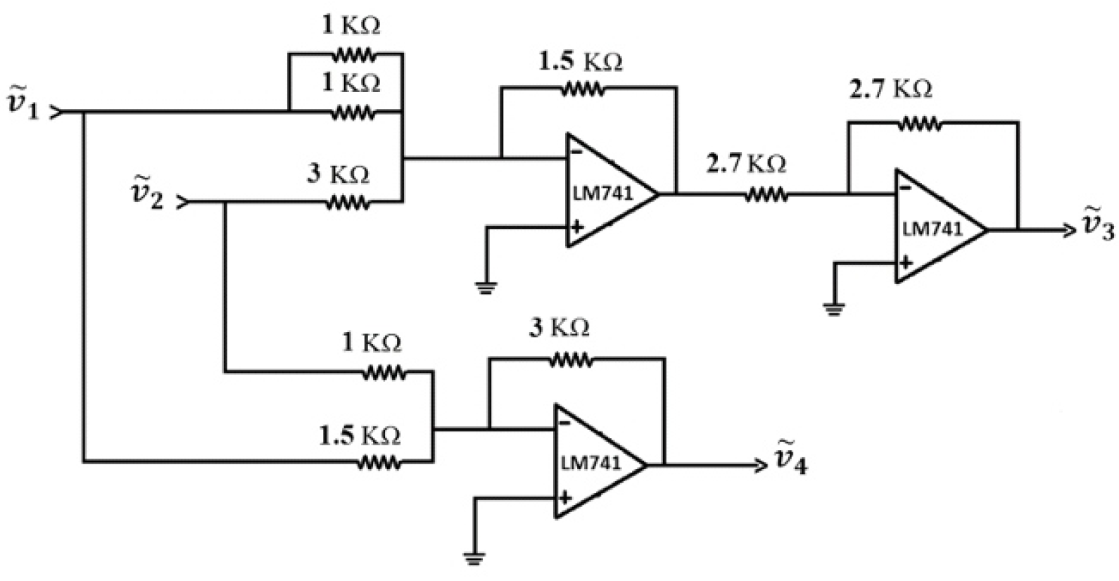
The authors of [10] considered the electrical circuit shown in Figure 1, where v 1 ˜ and v 2 ˜ are the input voltages, and v 3 ˜ and v 4 ˜ are the output voltages. The circuit is a kind of summing amplifier with two inputs and two outputs. The relationship between input and output voltages is as follows: 3 0.5 2 3 v 1 ˜ v 2 ˜ = v 3 ˜ v 4 ˜ .
They considered the output voltages as type-2 fuzzy numbers. In this paper, we treat the same example, but we consider the output voltages as intuitionistic fuzzy numbers, as considered by the authors in [7]:
v 3 ˜ = ( 14 + 2 α ; 14 2 α ; 16 3 α ; 16 + 3 α ) and
v 4 ˜ = ( 18 + 2 α ; 14 2 α ; 16 3 α ; 16 + 3 α ) .
Here, we are looking at how to calculate the input voltages when the output voltages are known but uncertain. That is, v 3 ˜ is “about 16 volts” and v 4 ˜ is “about –16 volts”. Different experts may have different viewpoints on the output voltage’s uncertainty.
Now, if we choose to focus on one expert’s interpretation, then the linear system shown in Equation (1) will be type-1 FLSE, as mentioned in [10].
In addition, we consider the hesitation of the expert, which is quite natural when making a decision, because of characteristics of human beings applying knowledge and skills. Then, the linear system shown in Equation (1) will be an intuitionistic fuzzy linear system of equations. This is more realistic than type-1 FLSE.
If we want to consider more than one expert’s opinion, then we obtain the system of equations as type-2 FLSE, originally considered in [10].
Now, if we consider different experts’ opinions individually, together with their hesitations, then we can take, for example, the arithmetic average of different IFNs to determine the output voltages, and the system can be better represented as IFLS.
In this case, the above system reduces to
3 v 1 ˜ + 0.5 v 2 ˜ = ( 14 + 2 α ; 18 2 α ; 16 3 α ; 16 + 3 α ) 2 v 1 ˜ 3 v 2 ˜ = ( 18 + 2 α ; 14 2 α ; 16 3 α ; 16 + 3 α )
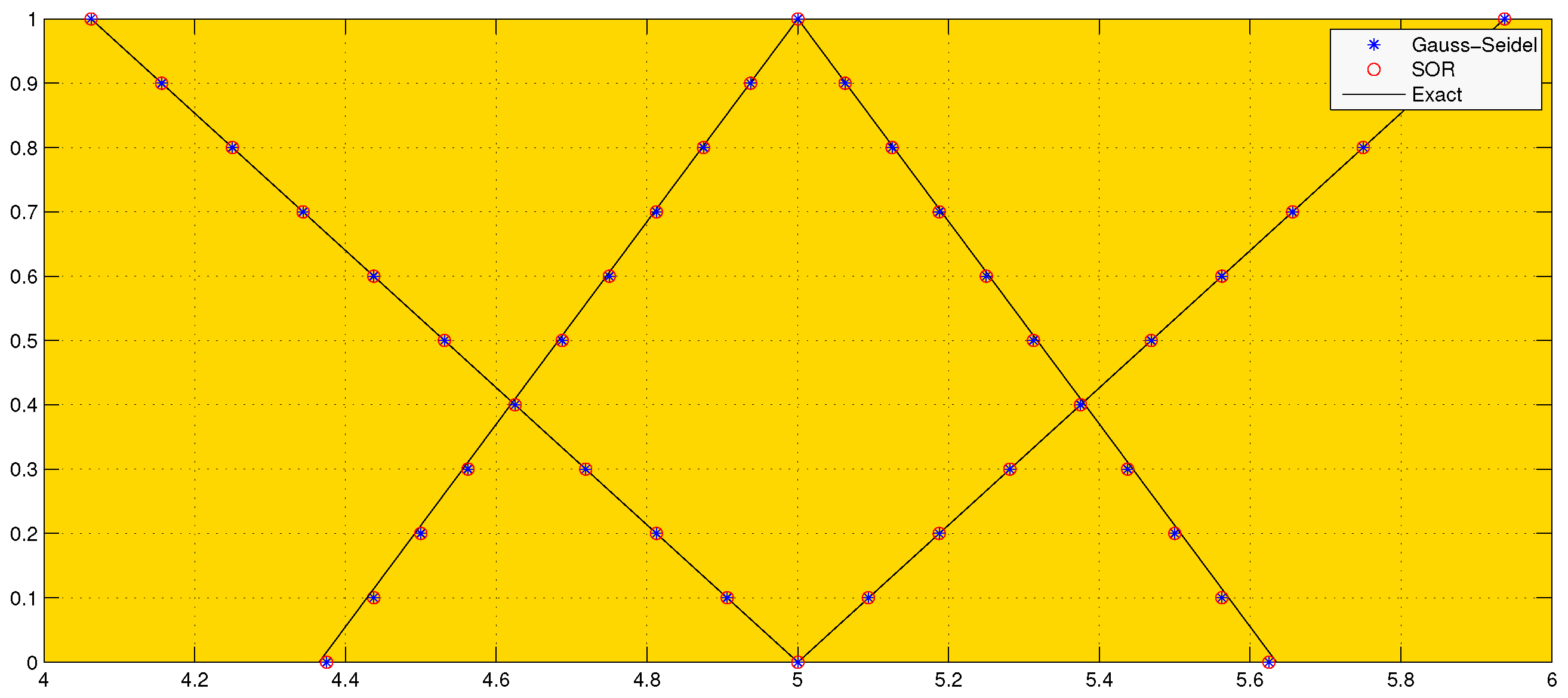
The exact and approximated solutions are plotted and compared for v 1 ˜ .
The exact and approximated solutions are plotted and compared for v 2 ˜ .

4. Conclusions

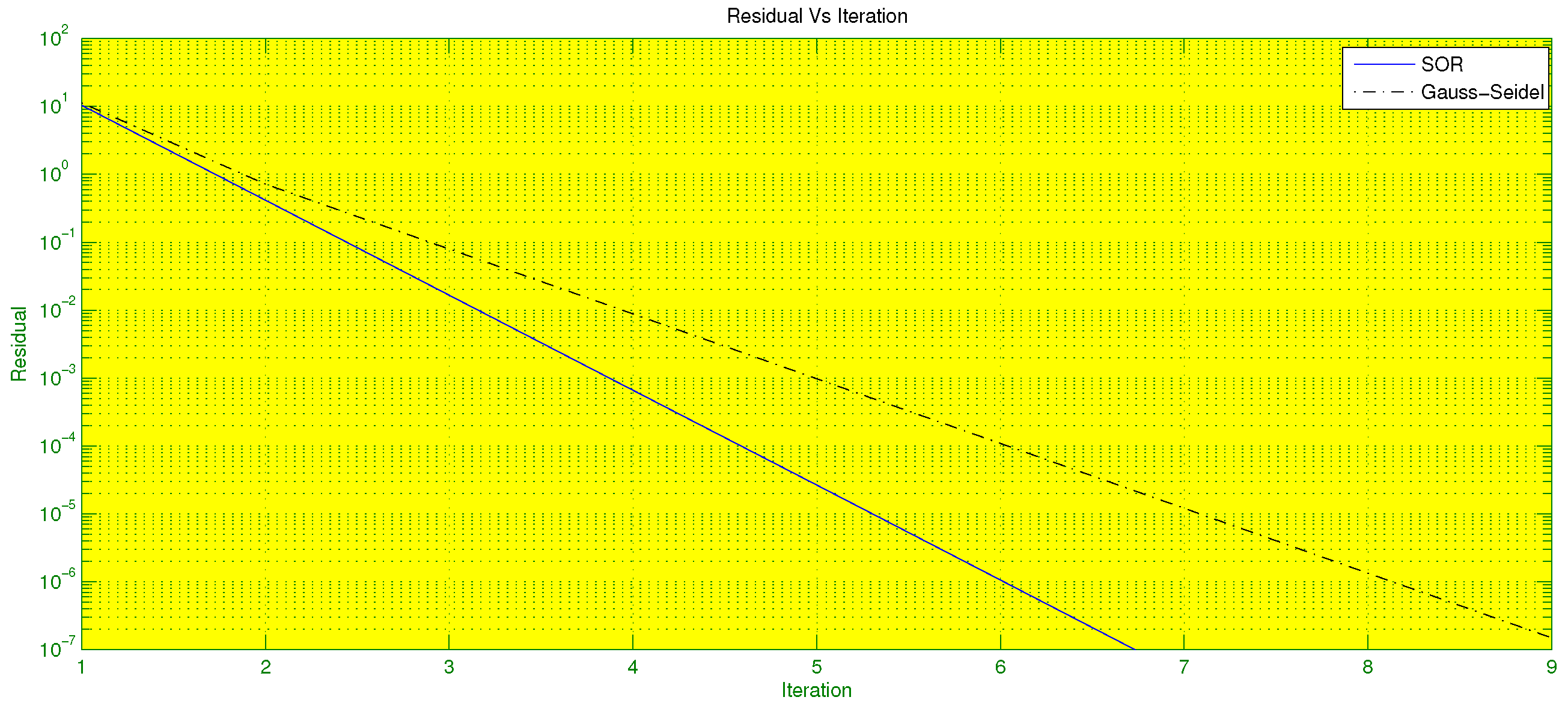
As can be seen in Figure 2 and Figure 3, the solutions obtained by both the methods for tolerance ϵ = 10 6 agreed quite well with the exact solution for both v 1 ˜ and v 2 ˜ . The convergence history in Figure 4 shows that the Gauss–Seidel method requires nine iterations and the SOR method requires eight iterations to converge in this case. As expected, the SOR method with w o p t = 0.9 is faster than the Gauss–Seidel method, even for this relatively small ( f o r n = 2 I F L S , i . e . , 8 × 8 c r i s p ) system of equations. Certainly, for large system of equations, convergence will be accelerated using the SOR method rather than the Gauss–Seidel method.
In future, we try to accelerate the convergence of the linear system using more efficient iterative methods, such as the Krylov subspace methods or Multigrid methods.

Author Contributions

All authors contributed equally to this work. All authors have read and agreed to the published version of the manuscript.

Funding

This research received no external funding.

Institutional Review Board Statement

Not applicable.

Informed Consent Statement

Not applicable.

Data Availability Statement

Enquiries about data availability should be directed to the authors.

Conflicts of Interest

The authors declare no conflict of interest.

References

  1. Zadeh, L.A. Fuzzy sets. Inf. Control 1965, 8, 338–353. [Google Scholar] [CrossRef]
  2. Atanassov, K.T. Intuitionistic fuzzy sets. Fuzzy Sets Syst. 1986, 20, 87–96. [Google Scholar] [CrossRef]
  3. Atanassov, K.T. Ideas for Intuitionistic Fuzzy Sets Equations, Inequations and Optimization. Notes Intuitionistic Fuzzy Sets 1995, 1, 17–24. [Google Scholar]
  4. Friedman, M.; Ming, M.; Kandel, A. Fuzzy linear systems. Fuzzy Sets Syst. 1998, 96, 201–209. [Google Scholar] [CrossRef]
  5. Allahviraloo, T. Numerical methods for fuzzy system of linear equations. Appl. Math. Comput. 2004, 155, 493–502. [Google Scholar]
  6. Allahviraloo, T. Successive over relaxation iterative method for fuzzy system of linear equations. Appl. Math. Comput. 2005, 162, 189–196. [Google Scholar]
  7. Atti, H.; Amma, B.B.; Melliani, S.; Chadli, S. Intuitionistic Fuzzy Linear Systems. In Intuitionistic and Type-2 Fuzzy Logic Enhancements in Neural and Optimization Algorithms: Theory and Applications, Studies in Computational Intelligence; Castillo, O., Melin, P., Kacprzyk, J., Eds.; Springer: Berlin/Heidelberg, Germany, 2020; Volume 862, pp. 133–144. [Google Scholar]
  8. Saw, B.C.; Man, S.; Bairagi, A.; Hazra, S.B. Iterative method for intuitionistic fuzzy system of linear equations. Soft Comput. 2023. submitted. [Google Scholar]
  9. Ortega, J.M. Numerical Analysis a Second Course; siam: Philadelphia, PA, USA, 1990. [Google Scholar]
  10. Najariyan, M.; Mazandarani, M.; John, R. Type-2 fuzzy linear systems. Granul. Comput. 2017, 6, 175–186. [Google Scholar] [CrossRef]
Figure 1. Electrical Circuit.
Csmf 07 00047 g001
Figure 2. Graphical representation of v 1 ˜ with continuous (exact solution) and approximate values for α = 0.0 , 0.1 , 0.2 , 0.3 , 0.4 , 0.5 , 0.6 , 0.7 , 0.8 , 0.9 , 1.0 for both Gauss–Seidel and SOR methods.
Csmf 07 00047 g002
Figure 3. Graphical representation of v 2 ˜ with continuous (exact solution) and approximate values for α = 0.0 , 0.1 , 0.2 , 0.3 , 0.4 , 0.5 , 0.6 , 0.7 , 0.8 , 0.9 , 1.0 for both Gauss–Seidel and SOR methods.
Csmf 07 00047 g003
Figure 4. Convergence history of Gauss–Seidel and SOR methods.
Csmf 07 00047 g004
Disclaimer/Publisher’s Note: The statements, opinions and data contained in all publications are solely those of the individual author(s) and contributor(s) and not of MDPI and/or the editor(s). MDPI and/or the editor(s) disclaim responsibility for any injury to people or property resulting from any ideas, methods, instructions or products referred to in the content.