The Burr XII Autoregressive Moving Average Model ^†

Abstract

The present work proposes a new class of model for random variables with support in the positive real line, this model explains the conditional quantile and is an alternative for modeling data that indicate asymmetric behavior and heavy tails. We present a new autoregressive moving average model based on the $\tau$–th quantile of the Burr XII distribution (BXII-ARMA) since the quantile is less sensitive than the average of heterogeneous populations and also suitable in the presence of outliers. This model makes it possible to model any quantile by a dynamic structure containing autoregressive terms and moving averages, time-varying regressors, unknown parameters, and a link function. The conditional maximum likelihood method is considered to estimate the parameters and build the confidence intervals of the BXII-ARMA model. In addition, the model is adjusted to real data related to the financial market and compared with other competing models.

1. Introduction

The origin of the Burr XII (BXII) distribution was through a system of distributions, which was introduced by [1]. The BXII was defined as the twelfth model of this system and has recently been applied mainly in income studies [2,3], poverty indicators [4,5], dropout proportion [6], and survival analysis [7,8], between others. For economists, the BXII is also well known as the Singh-Maddala distribution because it is widely used as an alternative to model income data [9]. In the methodological scope, some properties of the model were explored by [10,11,12]. Generalizations of the BXII distribution have also been explored in recent years, for example, the distributions Marshall-Olkin generalized Burr XII [13], Reflected Unit Burr XII [14], Generalized log-logistic Burr XII [13], and ${\mathrm{Burr}}_b^{SAR}$ distribution [15].

In recent literature, several types of research have been devoted to the development of time series models under the assumption of non-Gaussian distributions. Between them, ref. [16] developed the Generalized Autoregressive Moving Average (GARMA) models. In the GARMA approach, the conditional distribution of the fixed-time response variable t is modeled by a distribution belonging to the exponential family, and one of the most used generalization models is for positive series with Gamma distribution. After the proposal of the GARMA model by [16], proposing new models that are not based on a Gaussian structure was left aside. However, it has recently had an ascendancy in the literature, ref. [17] addressed an autoregressive moving average model based on the Rayleigh (RARMA) distribution for variables that assume values in positive reals. For variables that assume values in the range $(0,1)$, ref. [18] they formulated a Beta autoregressive moving average ($\beta$-ARMA) model, and in the studies of [19], the Kumaraswamy autoregressive moving average (KARMA) model was introduced.

In the context of forecasting, usual models have already been used to model financial market series to forecast economic indices [20], leasing value [21] and stock prices [22]. Articles on trading volume forecasts have also been published recently, in the stock market in India [23], ref. [24] in the real estate market. Therefore, time series analysis is a strategic tool used to predict future trends and moreover, it helps investors to make decisions that lead to good results and more profits.

The BXII is a distribution for random variables with support in the positive real line and has the ability to represent asymmetric behaviors and heavy tails. These characteristics make the BXII a suitable alternative both in survival analysis applications and in economic, hydrological, and environmental indicators. It is in this context that the present work is inserted, which aims to propose a new autoregressive moving average model based on a reparametrization in terms of the quantiles of the BXII distribution. This new class of model can help in the analysis and prediction of variables with these asymmetry characteristics.

2. The Burr XII ARMA Model

This section defines the BXII-ARMA model. For that purpose, we consider the parametrization of the BXII distribution proposed by [25], which is based on the quantities $\mu$ and $\tau$, where $\mu$ is the $\tau$–th quantile with $\tau \in (0,1)$ a known constant. This parameterization satisfies the relation $d=-log\left(1-\tau \right)/log\left(1+{\mu }^c\right)$. We provide a link to show the probability density function (pdf) forms that the reparameterized BXII can take (https://visionmt.shinyapps.io/RBXII/, accessed on 10 February 2023).

Let $Y_1,Y_2,\dots$ be a sequence of random variables, where each $Y_t$ ($t\in \mathbb{Z}$) assumes values $y_t\in {\mathbb{R}}^{+}$. Besides, let ${\mathcal{F}}_t$ be the $\sigma$-field generated by past observations $\{\dots ,y_{t-2},y_{t-1},y_t\}$ (i.e., the smallest $\sigma$-algebra such that the variables $Y_1,\dots ,Y_t$ are measurable). Additionally, suppose that each $Y_t$ conditional on previous information set ${\mathcal{F}}_{t-1}$ is distributed following a BXII law with parameters $c>0$ and ${\mu }_t$, where ${\mu }_t$ is the conditional $\tau$–th quantile of $Y_t$. Thus, the conditional pdf of $Y_t$ given ${\mathcal{F}}_{t-1}$ is

$$g\left(y_t|{\mathcal{F}}_{t-1}\right)=log\left(\frac{1}{1-\tau }\right)\frac{c{y}_t^{c-1}}{log\left(1+{\mu }_t^c\right)}{\left(1+y_t^c\right)}^{log\left(1-\tau \right)/log\left(1+{\mu }_t^c\right)-1},$$

(1)

and we denote as $Y_t|{\mathcal{F}}_{t-1}\sim$ BXII$({\mu }_t,c)$.

The conditional cumulative distribution function (cdf) and conditional quantile function (cqf) of $Y_t|{\mathcal{F}}_{t-1}$ are

$$\begin{array}{c}\hfill G\left(y_t|{\mathcal{F}}_{t-1}\right)=1-{\left(1+y_t^c\right)}^{log\left(1-\tau \right)/log\left(1+{\mu }_t^c\right)}\end{array}$$

(2)

and

$$\begin{array}{c}\hfill Q\left(u|{\mathcal{F}}_{t-1}\right)={\left[{\left(1-u\right)}^{log\left(1+{\mu }_t^c\right)/log\left(1-\tau \right)}-1\right]}^{1/c},\end{array}$$

respectively.

The h–th condition moment of $Y_t|{\mathcal{F}}_{t-1}$ can be expressed as

$$\mathrm{E}\left(Y_t^h\right|{\mathcal{F}}_{t-1})=-\frac{log\left(1-\tau \right)}{log\left(1+{\mu }_t^c\right)}\mathrm{B}\left(-\frac{log\left(1-\tau \right)}{log\left(1+{\mu }_t^c\right)}-h{c}^{-1},1+h{c}^{-1}\right),$$

where $h<c\left[-log\left(1-\tau \right)/log\left(1+{\mu }_t^c\right)\right]$ and $\mathrm{B}(·)$ is the Beta function.

The dynamic general BXII-ARMA model has the following specification for the $\tau$–th conditional quantile

$$\begin{array}{c}\hfill {\eta }_t=g\left({\mu }_t\right)=\alpha +x_t^{\top }\mathit{\beta }+\sum _{i=1}^p{\varphi }_i\left\{g\left(y_{t-i}\right)-x_{t-i}^{\top }\mathit{\beta }\right\}+\sum _{j=1}^q{\theta }_j{r}_{t-j},\end{array}$$

(3)

where ${\eta }_t$ is the linear predictor, $\alpha \in \mathbb{R}$ is a constant, ${\mathit{x}}_{\mathit{t}}$ denotes the k-dimensional vector containing the covariates at time t, $\mathit{\beta }={({\beta }_1,\cdots ,{\beta }_k)}^{\top }$ is a k-dimensional vector of unknown coefficients associated to the covariates, $g(·)$ is a strictly increasing and twice differentiable link function that relates the linear predictor to the $\tau$–th quantile. This function has important purposes in interpreting the response variable. The $r_t=g\left(y_t\right)-g\left({\mu }_t\right)$ term correspond to the random error; $\mathit{\varphi }={({\varphi }_1,\cdots ,{\varphi }_p)}^{\top },$ and $\mathit{\theta }={({\theta }_1,\cdots ,{\theta }_q)}^{\top }$ are the autoregressive and moving average coefficients, respectively.

3. Parameter Estimation

This section describes the estimation of the parameters of the model by conditional maximum likelihood method. Let $y_1,\dots ,y_n$ be the random sample satisfying the specification given by Equations (1) and (3) with $\delta ={(\alpha ,{\mathit{\beta }}^{\top },{\mathit{\varphi }}^{\top },{\mathit{\theta }}^{\top },c)}^{\top }$ denoting the $(2+k+p+q)$-dimensional parametric vector. The log-likelihood function of the BXII-ARMA model is expressed as

$$\begin{array}{c}\hfill \mathcal{l}=\mathcal{l}(\delta ;y_t|{\mathcal{F}}_{t-1})=\sum _{t=m+1}^n{\mathcal{l}}_t({\mu }_t,c),\end{array}$$

(4)

where

$$\begin{array}{cc}\hfill {\mathcal{l}}_t({\mu }_t,c)=& log\left[\frac{clog\left(\frac{1}{1-\tau }\right)}{log(1+{\mu }_t^c)}\right]+\left(c-1\right)log\left(y_t\right)+\left[\frac{log(1-\tau )}{log(1+{\mu }_t^c)}-1\right]log(1+y_t^c),\hfill \end{array}$$

${\mu }_t=g^{-1}\left({\eta }_t\right),$ and ${\eta }_t$ is defined in Equation (3). Note that Equation (4) holds, once ${\mathcal{l}}_t({\mu }_t,c)$ is null for the first $m=max(p,q)$ observations of $y_t$.

The conditional maximum likelihood estimators (CMLE), $\widehat{\delta }$ for $\delta$ are obtained through the maximization of Equation (4). Furthermore, the CMLE are obtained by equalizing the score vector to zero and solving the resulting system of equations. The calculations for the conditionals score vector and Fisher’s information matrix, and the construction of confidence intervals and hypothesis testings for the BXII-ARMA model were implemented in R programming language.

4. Numerical Results

This section presents an empirical application of the BXII-ARMA to datasets related to the financial market. Furthermore, the ARMA [26], GARMA [16], and RARMA [17] models are also fitted for comparative purposes. The function arima() is used to the ARMA fit. The implementation of the GARMA and RARMA models is similar to the BXII-ARMA model and is available in the PTSR package using the ptsr.fit() function. For more information, see [27]. The application is implemented in the R software. The dataset refers to the trading volume of the Banco Bradesco S.A. (BBD) stocks and was collected from the Yahoo Finance website (https://finance.yahoo.com/most-active (accessed on 10 February 2023)), which provides up-to-date financial news, international market data, including stock quotes, financial reports and original content. The information corresponds from 14 February 2022, to 10 February 2023, totaling 250 observations. The trading volume corresponds to the number of stocks bought and sold in a day, and the standard unit of these assets is given in U.S. Dollars (US$). Since trading volumes are usually large-scale numbers, we divided the series by one hundred million to better visualize the results. The last thirty observations of the series were removed to obtain the Mean Square Error (MSE), Mean Absolute Percentage Error (MAPE), and Mean Absolute Scaled Error (MASE) measures to choose the most accurate model. The forecast is estimated by one-step-ahead, updated by the actual value.

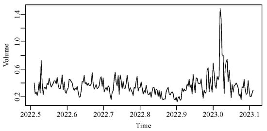
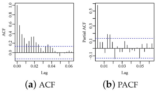
Figure 1 shows the graphs of the BBD trading volume serie. Figure 2 shows the autocorrelation function (ACF) and partial autocorrelation (PACF) plots of the BBD trading volume. Figure 2a, it is noted that the vast majority of observations are outside the confidence interval (CI). In the PACF, shown in Figure 2b, almost all observations are within the CI. The series was identified as stationary through the unit root tests, Phillips-Perron (PP) and Kwiatkowski-Phillips-Schmidt-Shin (KPSS) with p-values equal to $0.01$ and $0.1$, respectively. Thus, the ARMA, GARMA, RARMA, and BXII-ARMA models were adjusted to choose the model that best represented the behavior of the studied serie. The best fit of each model class is selected through the AIC, BIC, and HQ measures. After, the best fit of each class, the model with the best prediction is chosen.

Figure 1. Time series plot of BBD trading volume.

Figure 2. ACF and PACF of BBD trading volume.

Table 1 shows the fit of the models with the parameter estimates, the standard errors (SE), and the p-values of each estimate. The structure for the BBD trading volume is given by one autoregressive coefficient and four moving average filters, namely ARMA(1,4), GARMA(1,4), RARMA(1,4), and BXII-ARMA(1,4). For the ARMA model, only the intercept was significant. For the GARMA and RARMA models, all coefficients were significant, except for the autoregressive ${\varphi }_1$ and the moving average coefficient ${\theta }_4$. All coefficients of the BXII-ARMA model were significant at the $5\%$ significance level. Table 2 presents the adequacy measures adopted as methodologies for comparing forecast performance between the different best-fitted models in each class. Therefore, the MSE, MAPE, and MASE measurements are calculated for all models, considering the thirty-day out-of-sample estimates with the last thirty observations taken from the series. Therefore, the best results of the accurate measurements are given by the BXII-ARMA model for the data sets.

Table 1. ARMA, GARMA, RARMA, and BXII-ARMA adjustments in the time serie.

ARMA(1,4)				GARMA(1,4)
Coef.	Estimate	SE	p-Value	Coef.	Estimate	SE	p-Value
Int.	0.3558	0.0189	0.0000	$\alpha$	$-1.0887$	0.1188	0.0000
${\varphi }_1$	$-0.2537$	2.4091	0.9161	${\varphi }_1$	$-0.0280$	0.0971	0.7730
${\theta }_1$	0.8051	2.4058	0.7379	${\theta }_1$	1.4578	0.1434	0.0000
${\theta }_2$	0.5003	1.3250	0.7057	${\theta }_2$	1.0380	0.2281	0.0000
${\theta }_3$	0.4213	0.8648	0.6261	${\theta }_3$	1.0413	0.1716	0.0000
${\theta }_4$	0.0881	0.7846	0.9106	${\theta }_4$	$-0.0078$	0.1746	0.9640
_	_	_	_	$\phi$	11.5539	1.0861	0.0000
RARMA(1,4)				BXII-ARMA(1,4)
Coef.	Estimate	SE	p-Value	Coef.	Estimate	SE	p-Value
$\alpha$	$-1.3357$	0.1799	0.0000	$\alpha$	$-0.6286$	0.0880	0.0000
${\varphi }_1$	0.3683	0.5293	0.4866	${\varphi }_1$	0.3398	0.0663	0.0000
${\theta }_1$	1.2574	0.3980	0.0016	${\theta }_1$	0.3705	0.0541	0.0000
${\theta }_2$	1.0528	0.4046	0.0093	${\theta }_2$	0.2454	0.0651	0.0002
${\theta }_3$	1.1475	0.3057	0.0002	${\theta }_3$	0.2801	0.0611	0.0000
${\theta }_4$	$-0.0185$	0.3283	0.9549	${\theta }_4$	0.2361	0.0626	0.0002
_	_	_	_	c	3.7013	0.1806	0.0000

Table 2. Forecasting performance comparison among different the best fitted models in each class.

Model	MSE	MAPE	MASE
ARMA	0.0555	0.4233	0.8224
GARMA	0.0567	0.4129	0.8215
RARMA	0.0676	0.3834	0.8679
BXII-ARMA	0.0071	0.1491	0.3020

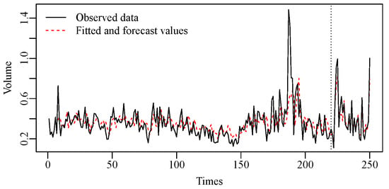
Figure 3 shows the residuals BXII-ARMA(1,4) plots to the BBD trading volume. In Figure 3a, the quantile residuals show the absence of the tendency, and their behavior is similar to white noise. Figure 3b,c, have the ACF and PACF of the residuals that confirm that they are similar to white noise. Figure 4 provides a plot of the actual and adjusted values. Figure 4 shows the observed and adjusted values of the BBD trading volume. All analyzed graphs show that BXII-ARMA models adjusted to BBD trading volume can be used to make step-ahead predictions of the considered sample.

Figure 3. Residual diagnostic plots of the fitted BXII-MA(1,4) model for the trading volume of BBD.

Figure 4. Observed and adjusted values of the BXII-ARMA model.

5. Concluding Remarks

This study proposes an autoregressive moving averages model based on a quantile parameterization of the BXII distribution. We carried out an economic application using the trading volume of Banco Bradesco stock to verify the adequacy of the proposed model. The proposed model is compared with other models of time series to verify its goodness of fit to the dataset used. We show some results for the mathematical properties of the proposed model, such as conditional moments and probability density, cumulative distribution, and conditional quantile functions. In addition, we estimated the model’s parameters by the maximum likelihood method. An application of time series was carried out using a real dataset, referring to the BBD trading volume, and BXII-ARMA(1,4) was fitted The BXII-ARMA model was adjusted to the data and the predicted values were obtained close to the real values of the series. It was also verified that, through the MSE, MAPE, and MASE measures, the BXII-ARMA model surpassed the ARMA, GARMA, and RARMA models, being a useful and flexible alternative for the adjustment of non-negative time series and with asymmetric patterns. Thus, the BXII-ARMA model is adequate to satisfactorily capture the dynamics of Banco Bradesco trading volume. It should be noted that the BXII-ARMA is a new methodology whose applicability can be extended to other topics.

References

- Burr, I.W. Cumulative frequency functions. Ann. Math. Stat. 1942, 13, 215–232. [Google Scholar] [CrossRef]
- Bhatti, F.A.; Hamedani, G.G.; Korkmaz, M.Ç.; Sheng, W.; Ali, A. On the Burr XII-moment exponential distribution. PLoS ONE 2021, 16, e0246935. [Google Scholar] [CrossRef] [PubMed]
- Guerra, R.R.; Peña-Ramírez, F.A.; Cordeiro, G.M. The Weibull Burr XII distribution in lifetime and income analysis. An. Acad. Bras. Ciências 2021, 93, 1–28. [Google Scholar] [CrossRef] [PubMed]
- Dhongde, S.; Minoiu, C. Global poverty estimates: A sensitivity analysis. World Dev. 2013, 44, 1–13. [Google Scholar] [CrossRef]
- Thompson, B.S. Empirical likelihood-based inference for poverty measures with relative poverty lines. Econom. Rev. 2013, 32, 513–523. [Google Scholar] [CrossRef]
- Ribeiro, T.F.; Peña-Ramírez, F.A.; Guerra, R.R.; Cordeiro, G.M. Another unit Burr XII quantile regression model based on the different reparameterization applied to dropout in Brazilian undergraduate courses. PLoS ONE 2022, 17, e0276695. [Google Scholar] [CrossRef]
- Low, V.J.M.; Khoo, H.L.; Khoo, W.C. Statistical modelling of bus travel time with Burr distribution. Itm Web Conf. 2021, 36, 1–15. [Google Scholar] [CrossRef]
- Ramires, T.G.; Nakamura, L.R.; Righetto, A.J.; Carvalho, R.J.; Vieira, L.A.; Pereira, C.A. Comparison between Highly Complex Location Models and GAMLSS. Entropy 2021, 23, 469. [Google Scholar] [CrossRef]
- Singh, S.K.; Maddala, G.S. A function for the size distribution of incomes. Econometrica 1976, 44, 963–970. [Google Scholar] [CrossRef]
- Tadikamalla, P.R. A Look at the Burr and Related Distribution. Int. Stat. Rev. Int. Stat. 1980, 48, 337–344. [Google Scholar] [CrossRef]
- Zimmer, W.J.; Keats, J.B.; Wang, F.K. The Burr XII distribution in reliability analysis. J. Qual. Technol. 1998, 30, 386–394. [Google Scholar] [CrossRef]
- Watkins, A. A note on expected Fisher information for the Burr XII distribution. Microelectron. Reliab. 1997, 37, 1849–1852. [Google Scholar] [CrossRef]
- Muse, A.H.; Mwalili, S.; Ngesa, O.; Almalki, S.J.; Abd-Elmougod, G.A. Bayesian and classical inference for the generalized log-logistic distribution with applications to survival data. Comput. Intell. Neurosci. 2021, 2021, 1–24. [Google Scholar] [CrossRef]
- Ribeiro, T.F.; Cordeiro, G.M.; Peña-Ramírez, F.A.; Guerra, R.R. A new quantile regression for the COVID-19 mortality rates in the United States. Comput. Appl. Math. 2021, 40, 1–16. [Google Scholar] [CrossRef]
- Sagrillo, M.; Guerra, R.R.; Machado, R.; Bayer, F.M. A generalized control chart for anomaly detection in SAR imagery. Comput. Ind. Eng. 2023, 177, 109030. [Google Scholar] [CrossRef]
- Benjamin, M.A.; Rigby, R.A.; Stasinopoulos, D.M. Generalized autoregressive moving average models. J. Am. Stat. Assoc. 2003, 98, 214–223. [Google Scholar] [CrossRef]
- Bayer, F.M.; Bayer, D.M.; Marinoni, A.; Gamba, P. A Novel Rayleigh Dynamical Model for Remote Sensing Data Interpretation. IEEE Trans. Geosci. Remote Sens. 2020, 58, 4989–4999. [Google Scholar] [CrossRef]
- Cribari-Neto, F.; Scher, V.T.; Bayer, F.M. Beta autoregressive moving average model selection with application to modeling and forecasting stored hydroelectric energy. Int. J. Forecast. 2023, 39, 98–109. [Google Scholar] [CrossRef]
- Melchior, C.; Zanini, R.R.; Guerra, R.R.; Rockenbach, D.A. Forecasting Brazilian mortality rates due to occupational accidents using autoregressive moving average approaches. Int. J. Forecast. 2021, 37, 825–837. [Google Scholar] [CrossRef]
- Jeong, Y.; Lee, S. Recurrent neural network-adapted nonlinear ARMA-GARCH model with application to S&P 500 index data. Korean Data Inf. Sci. Soc. 2019, 30, 1187–1195. [Google Scholar]
- Korbi, A.; Lleshaj, L. Finance leasing and arma forecasting: Evidence from albania. Eur. J. Bus. Manag. Res. 2020, 5, 1–6. [Google Scholar] [CrossRef]
- Koh, W.S.; Heng, H.S.; Wong, C.Z.; Lai, P.L.; Dass, C. Forecasting Stock Price using ARMA Model. INTI J. 2020, 2020, 1–8. [Google Scholar]
- Shah, H.; Bhatt, V.; Shah, J. A Neoteric Technique Using ARIMA-LSTM for Time Series Analysis on Stock Market Forecasting. In Proceedings of the Mathematical Modeling, Computational Intelligence Techniques and Renewable Energy: Proceedings of the Second International Conference, MMCITRE 2021, Gandhinagar, India, 6–8 February 2021; Springer: Singapore, 2022; pp. 381–392. [Google Scholar]
- Lee, C.; Park, K.K.H. Forecasting trading volume in local housing markets through a time-series model and a deep learning algorithm. Eng. Constr. Archit. Manag. 2022, 29, 165–178. [Google Scholar] [CrossRef]
- Araújo, F.J.M.; Guerra, R.R.; Peña-Ramírez, F.A. The Burr XII quantile regression for salary-performance models with applications in the sports economy. Comput. Appl. Math. 2022, in press. [Google Scholar] [CrossRef]
- Box, G.E.; Jenkins, G.M. Time Series Analysis Forecasting and Control; Department of Statistics, University of Wisconsin Madison: Madison, WI, USA, 1970; pp. 1–574. [Google Scholar]
- Prass, T.S.; Carlos, J.H.; Taufemback, C.G.; Pumi, G. Positive Time Series Regression Models. arXiv 2022, arXiv:2201.03667. [Google Scholar]
Disclaimer/Publisher’s Note: The statements, opinions and data contained in all publications are solely those of the individual author(s) and contributor(s) and not of MDPI and/or the editor(s). MDPI and/or the editor(s) disclaim responsibility for any injury to people or property resulting from any ideas, methods, instructions or products referred to in the content. |
© 2023 by the authors. Licensee MDPI, Basel, Switzerland. This article is an open access article distributed under the terms and conditions of the Creative Commons Attribution (CC BY) license (https://creativecommons.org/licenses/by/4.0/).