
Quantifying Bias in a Face Verification System †

 ,
,
Abstract
:1. Introduction
2. Related Work
2.1. Sources of Bias
2.2. Statistical Fairness Definitions
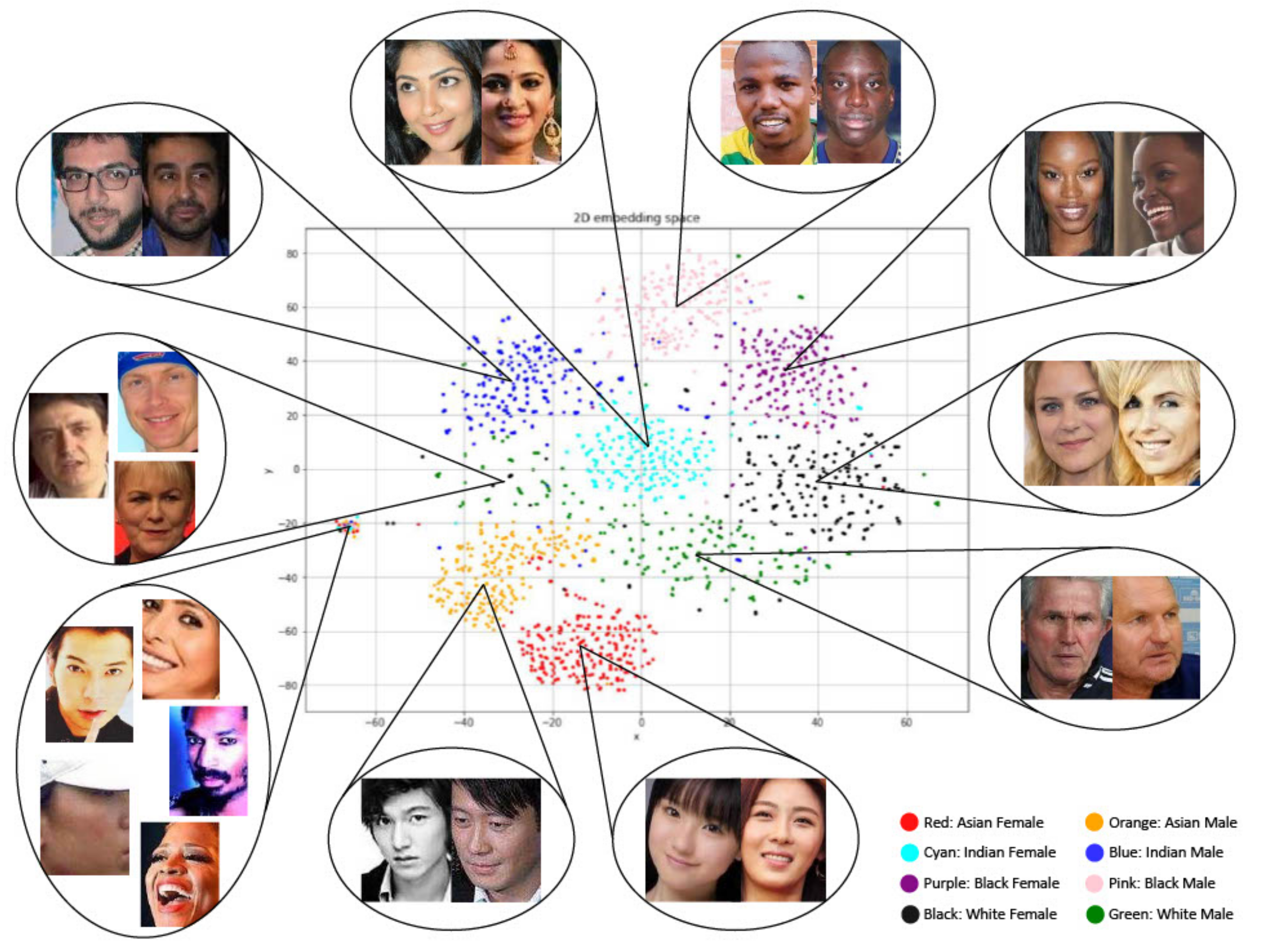
2.3. Bias in the Embedding Space
3. Method
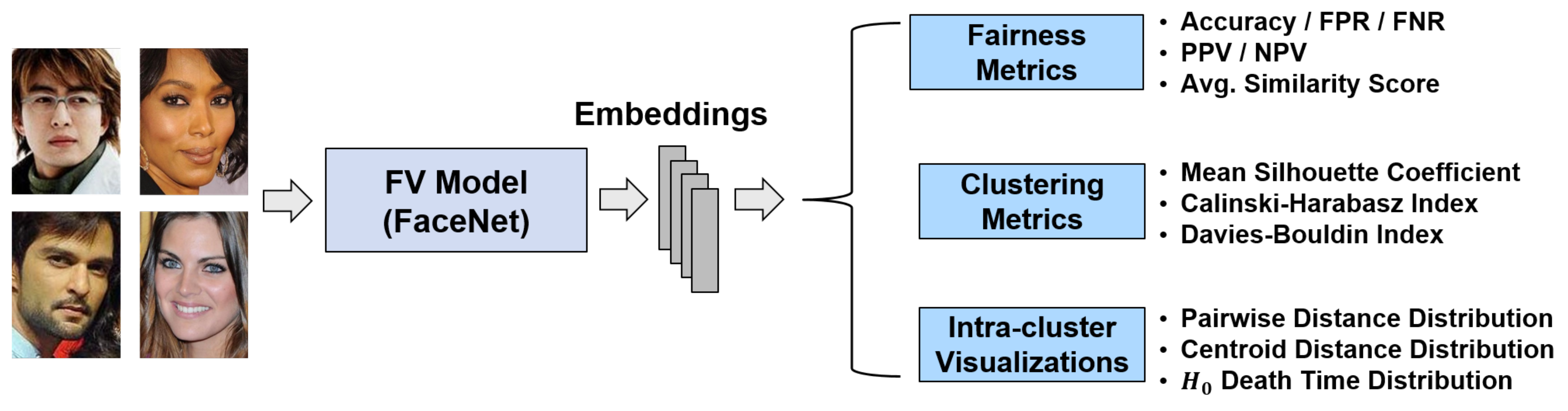
3.1. FV Pipeline
- Pass a pair of face images to MTCNN to crop them to bounding boxes around the faces (we discard data where MTCNN detects no faces). Each input pair has an “actual classification” of 1 (genuine) or 0 (imposter).
- Pass each cropped image tensor into the model (FaceNet, for our experiments) to produce two face embeddings.
- Compute the cosine similarity between the two embeddings (the “similarity score”).
- Use a pre-determined threshold (the threshold is determined according to a false accept rate (FAR) of 0.05 on a 20% heldout validation set; all datasets have no overlap between people in the testing and validation splits) to produce a “predicted classification” of 1 (genuine) or 0 (imposter).
3.2. Datasets
3.3. Statistical Fairness
3.4. Cluster-Based Fairness
- Mean silhouette coefficient [37]: A value in the range [−1, 1] indicating how similar elements are to their own cluster. A higher value indicates that elements are more similar to their own cluster and less similar to other clusters (good clustering).
- Calinski–Harabasz index [38]: The ratio of between-cluster variance and within-cluster variance. A larger index means greater separation between clusters and less within clusters (good clustering).
- Davies–Bouldin index [39]: A value greater than or equal to zero aggregating the average similarity measure of each cluster with its most similar cluster, judging cluster separation according to their dissimilarity (a lower index means better clustering).
4. Experiments
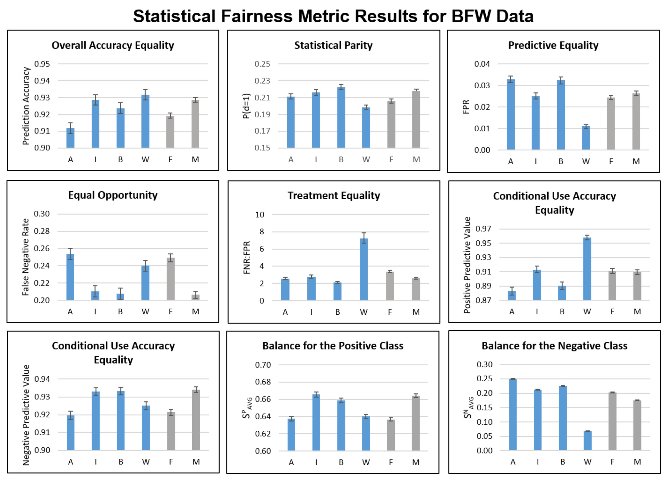
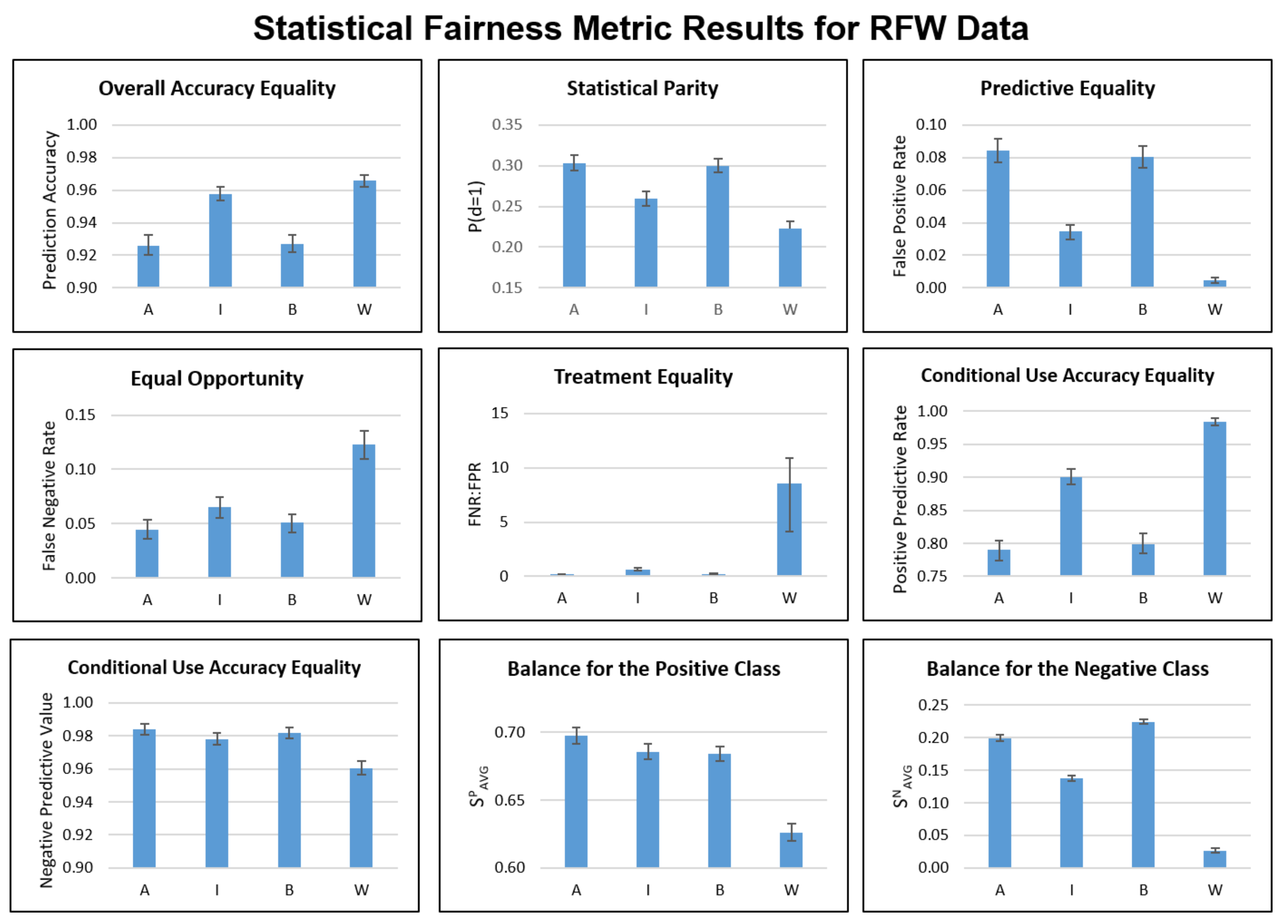
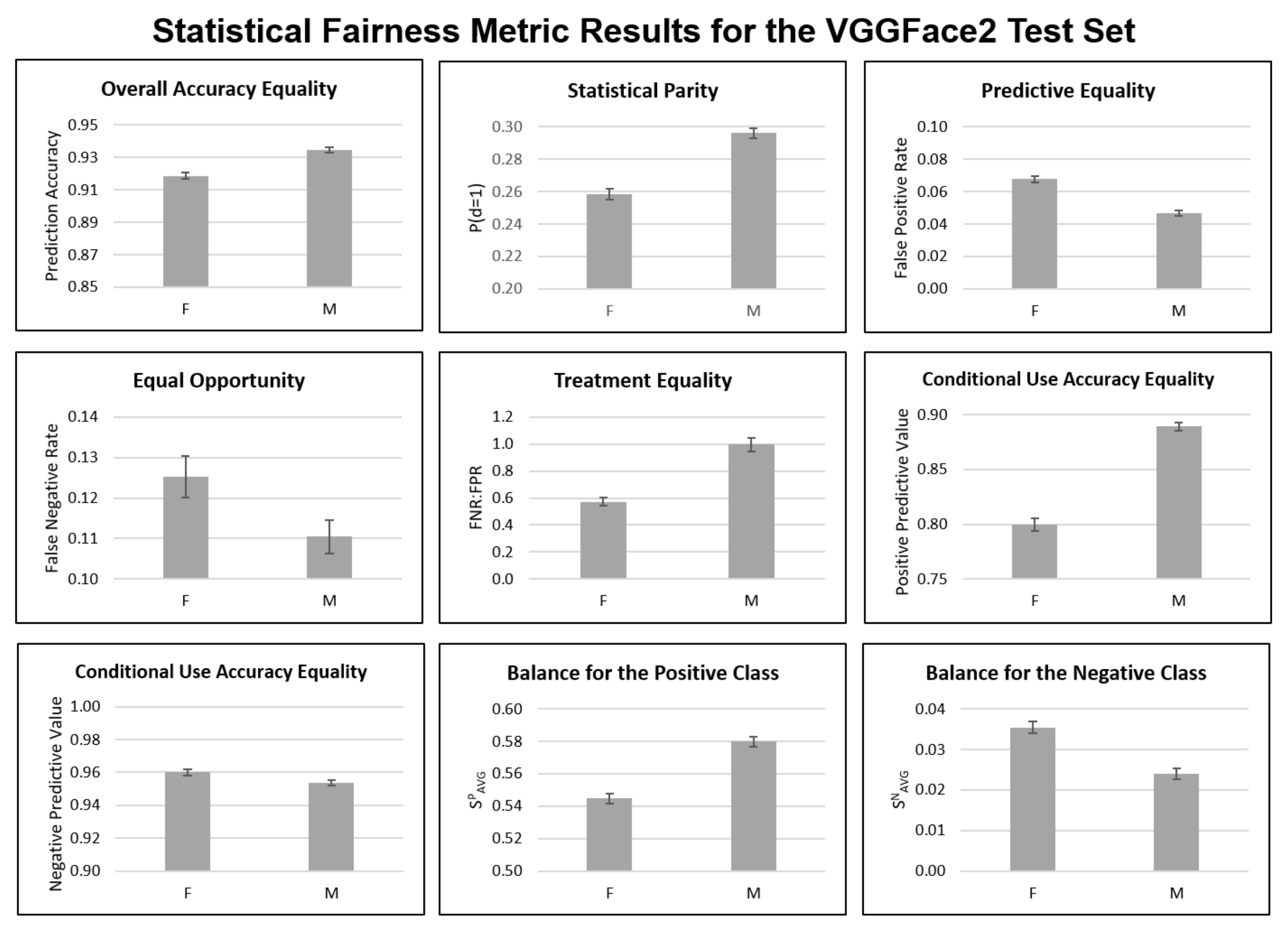
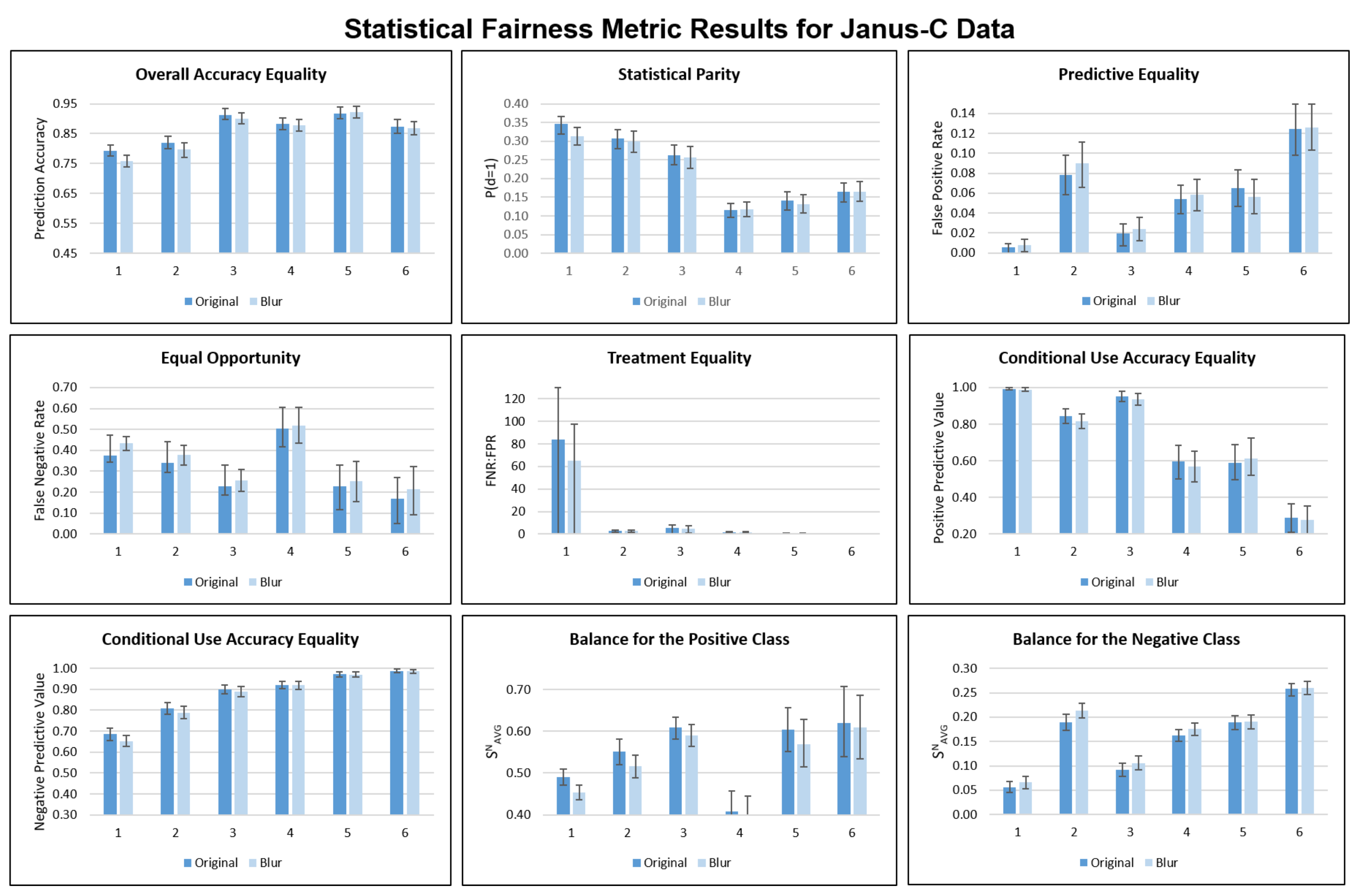
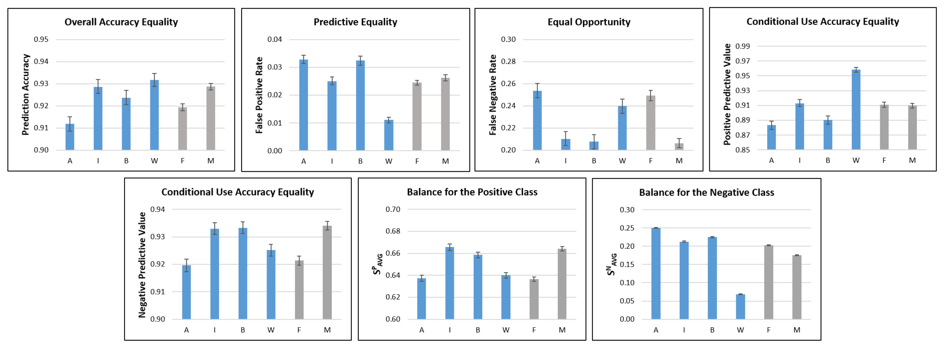
4.1. Statistical Fairness Metrics
4.2. Clustering Metrics
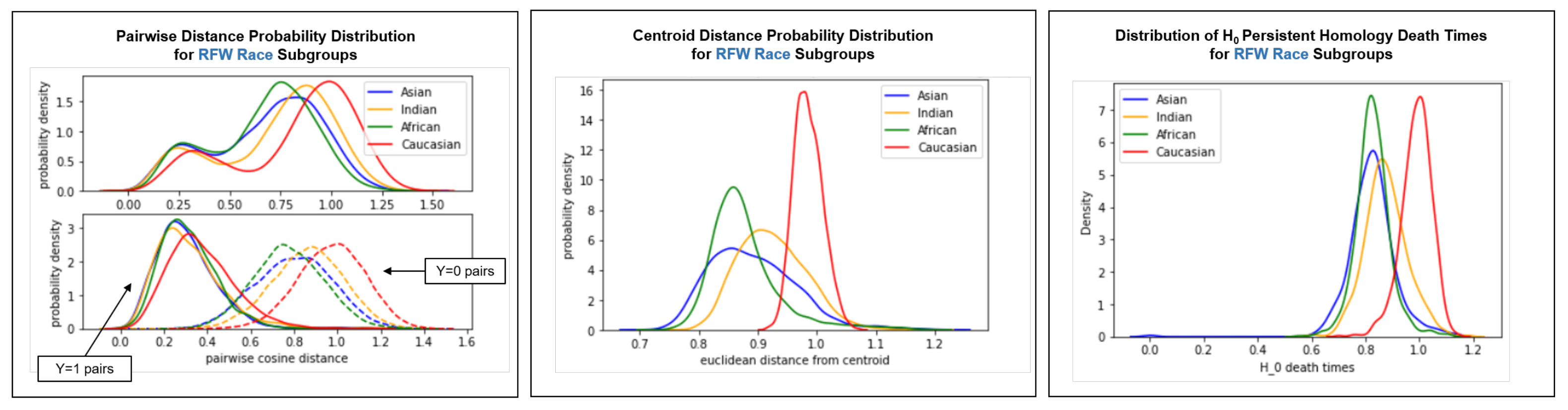
4.3. Intra-Cluster Fairness Visualizations
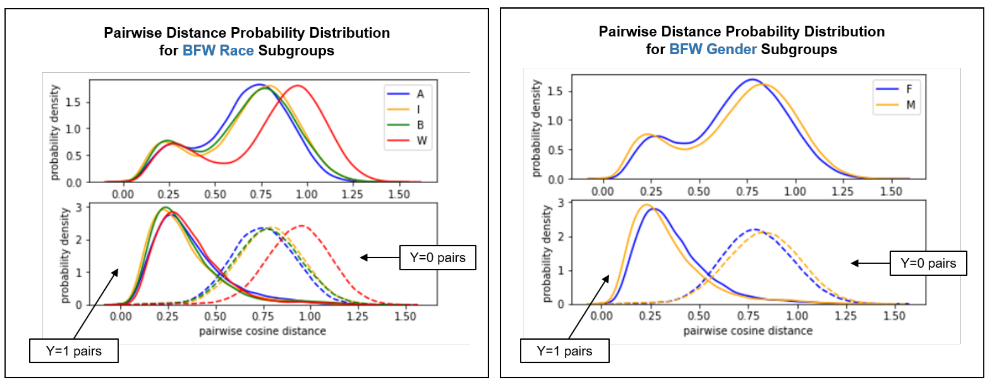
4.3.1. Pairwise Distance Distribution
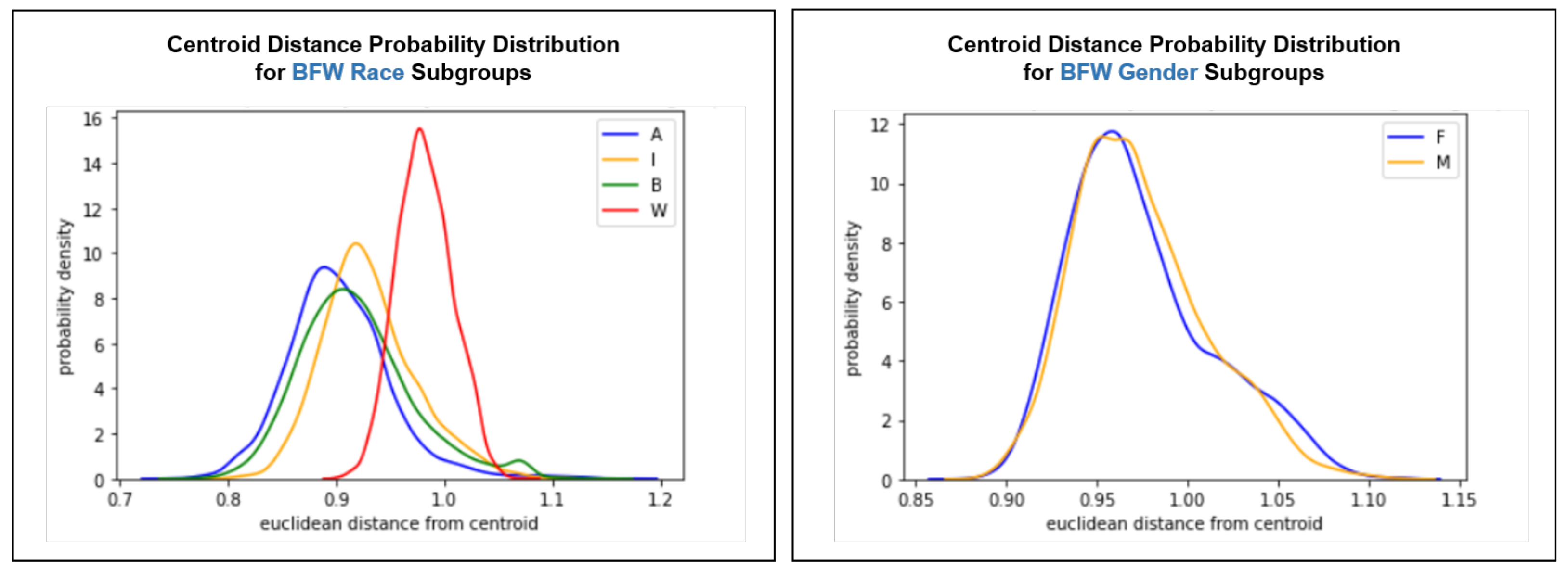
4.3.2. Centroid Distance Distribution
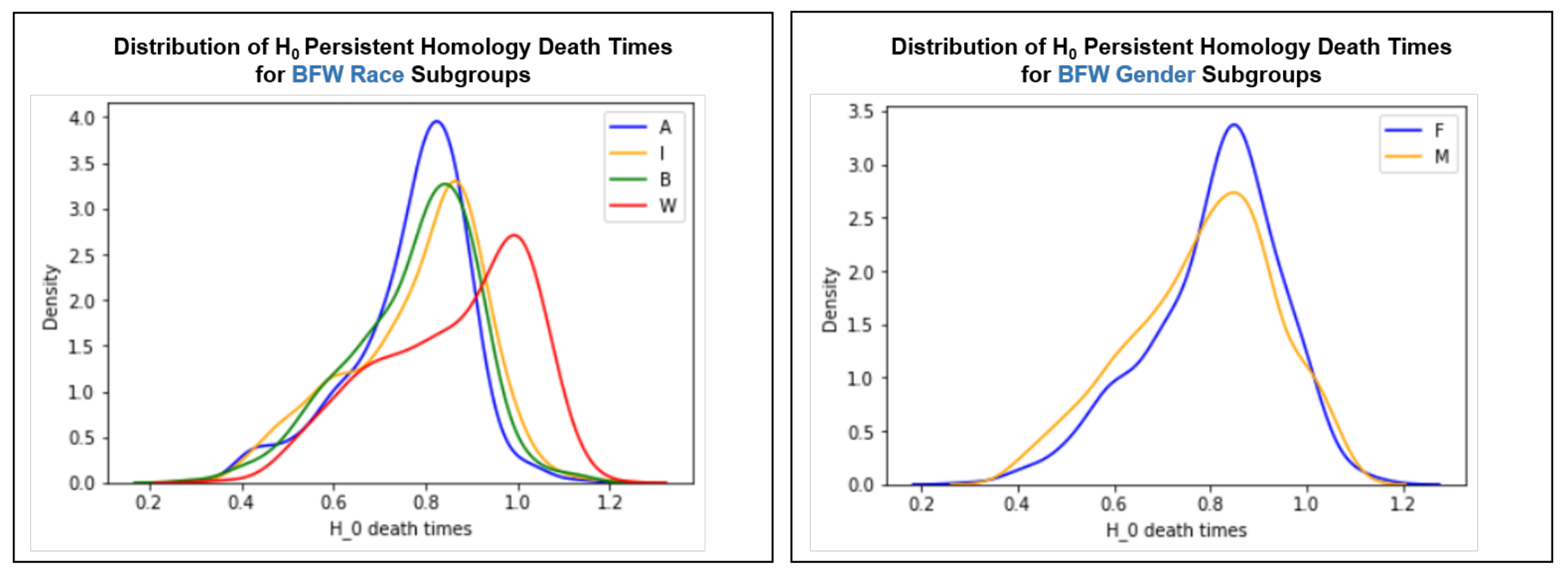
4.3.3. Persistent Homology
5. Conclusions
Author Contributions
Funding
Institutional Review Board Statement
Informed Consent Statement
Data Availability Statement
Acknowledgments
Conflicts of Interest
Abbreviations
| BFW | Balanced Faces in the Wild |
| CH | Calinski–Harabasz Index |
| DB | Davies–Bouldin Index |
| FNR | False Negative Rate |
| FPR | False Positive Rate |
| FR | Face Recognition |
| FV | Face Verification |
| IJBC | IARPA Janus Benchmark C |
| ML | Machine Learning |
| MS | Mean Silhouette Coefficient |
| MTCNN | Multi-Task Cascaded Convolutional Networks |
| NPV | Negative Predictive Value |
| PPV | Positive Predictive Value |
| RFW | Racial Faces in the Wild |
| t-SNE | t-distributed Stochastic Neighbor Embedding |
Appendix A. Pair Generation

| Asian | Indian | Black | White | |
|---|---|---|---|---|
| % positive | 25.0 | 25.0 | 25.2 | 25.0 |
| % negative | 75.0 | 75.0 | 74.8 | 75.0 |
| Female | 1 | 2 | 3 | 4 | 5 | 6 |
|---|---|---|---|---|---|---|
| % positive | 54.9 | 40.6 | 36.5 | 14.9 | 14.4 | 7.1 |
| % negative | 45.1 | 59.4 | 63.5 | 85.1 | 85.6 | 92.9 |
| Male | 1 | 2 | 3 | 4 | 5 | 6 |
| % positive | 54.7 | 37.3 | 29.5 | 13.7 | 8.6 | 5.5 |
| % negative | 45.3 | 62.7 | 70.5 | 86.3 | 91.4 | 94.5 |

| Female | Male | |
|---|---|---|
| % positive | 23.6 | 29.6 |
| % negative | 76.4 | 70.4 |
Appendix B. Statistical Fairness Metric Experiments


Appendix C. Clustering Metrics
| Metric | Race |
|---|---|
| MS↑ | 0.112 |
| CH↑ | 1423 |
| DB↓ | 4.21 |
| Metric | Gender |
|---|---|
| MS↑ | 0.026 |
| CH↑ | 1835 |
| DB↓ | 8.44 |
| Metric | Gender | Skin Tone |
|---|---|---|
| MS↑ | 0.034 | −0.002 |
| CH↑ | 380 | 227 |
| DB↓ | 7.57 | 7.81 |
Appendix D. Clustering Visualizations


Intra-Cluster Distribution T-Tests
| Pairwise Distance Distributions | Centroid Distance Distributions | Death Time Distributions | |||||||||
|---|---|---|---|---|---|---|---|---|---|---|---|
| I | B | W | I | B | W | I | B | W | |||
| A | <0.001 | <0.001 | <0.001 | A | <0.001 | <0.001 | <0.001 | A | >0.999 | >0.999 | <0.001 |
| I | - | <0.001 | <0.001 | I | - | <0.001 | <0.001 | I | - | >0.999 | <0.001 |
| B | - | - | <0.001 | B | - | - | <0.001 | B | - | - | <0.001 |
| Pairwise Distance Distributions | Centroid Distance Distributions | Death Time Distributions | |||||||||
| M | M | M | |||||||||
| F | <0.001 | F | >0.999 | F | >0.03 | ||||||
| Pairwise Distance Distributions | Centroid Distance Distributions | Death Time Distributions | |||||||||
|---|---|---|---|---|---|---|---|---|---|---|---|
| I | B | W | I | B | W | I | B | W | |||
| A | <0.001 | <0.001 | <0.001 | A | <0.001 | <0.001 | <0.001 | A | <0.001 | >0.999 | <0.001 |
| I | - | <0.001 | <0.001 | I | - | <0.001 | <0.001 | I | - | <0.001 | <0.001 |
| B | - | - | <0.001 | B | - | - | <0.001 | B | - | - | <0.001 |
| Pairwise Distance Distributions | Centroid Distance Distributions | Death Time Distributions | |||
|---|---|---|---|---|---|
| M | M | M | |||
| F | <0.001 | F | <0.001 | F | 0.02 |
| Pairwise Distance Distributions | Centroid Distance Distributions | Death Time Distributions | |||||||||||||||
|---|---|---|---|---|---|---|---|---|---|---|---|---|---|---|---|---|---|
| 2 | 3 | 4 | 5 | 6 | 2 | 3 | 4 | 5 | 6 | 2 | 3 | 4 | 5 | 6 | |||
| 1 | >0.999 | >0.999 | 0.01 | 0.62 | >0.999 | 1 | <0.001 | <0.001 | <0.001 | <0.001 | <0.001 | 1 | <0.001 | 0.81 | >0.999 | 0.13 | <0.001 |
| 2 | - | 0.70 | <0.001 | 0.02 | >0.999 | 2 | - | <0.001 | <0.001 | >0.999 | <0.001 | 2 | - | <0.001 | <0.001 | 0.22 | >0.999 |
| 3 | - | - | 0.30 | >0.999 | 0.54 | 3 | - | - | <0.001 | <0.001 | <0.001 | 3 | - | - | 0.98 | 0.03 | <0.001 |
| 4 | - | - | - | 0.91 | <0.001 | 4 | - | - | - | <0.001 | <0.001 | 4 | - | - | - | 0.98 | 0.06 |
| 5 | - | - | - | - | 0.003 | 5 | - | - | - | - | <0.001 | 5 | - | - | - | - | 0.99 |
| Pairwise Distance Distributions | Centroid Distance Distributions | Death Time Distributions | |||||||||||||||
| M | M | M | |||||||||||||||
| F | 0.08 | F | >0.999 | F | >.999 | ||||||||||||
References
- Monahan, J.; Skeem, J.L. Risk Assessment in Criminal Sentencing. Annu. Rev. Clin. Psychol. 2016, 12, 489–513. [Google Scholar] [CrossRef] [PubMed] [Green Version]
- Christin, A.; Rosenblat, A.; Boyd, D. Courts and Predictive Algorithms. Data & Civil Rights: A New Era of Policing and Justice. 2016. Available online: https://www.law.nyu.edu/sites/default/files/upload_documents/Angele%20Christin.pdf (accessed on 28 February 2022).
- Romanov, A.; De-Arteaga, M.; Wallach, H.; Chayes, J.; Borgs, C.; Chouldechova, A.; Geyik, S.; Kenthapadi, K.; Rumshisky, A.; Kalai, A.T. What’s in a Name? Reducing Bias in Bios without Access to Protected Attributes. arXiv 2019, arXiv:1904.05233. [Google Scholar]
- De-Arteaga, M.; Romanov, A.; Wallach, H.; Chayes, J.; Borgs, C.; Chouldechova, A.; Geyik, S.; Kenthapadi, K.; Kalai, A.T. Bias in Bios: A Case Study of Semantic Representation Bias in a High-Stakes Setting. In Proceedings of the Conference on Fairness, Accountability, and Transparency, Atlanta, GA, USA, 29–31 January 2019. [Google Scholar]
- Fuster, A.; Goldsmith-Pinkham, P.; Ramadorai, T.; Walther, A. Predictably Unequal? The Effects of Machine Learning on Credit Markets. SSRN Electron. J. 2017, 77, 5–47. [Google Scholar] [CrossRef]
- Mitchell, S.; Potash, E.; Barocas, S.; D’Amour, A.; Lum, K. Prediction-Based Decisions and Fairness: A Catalogue of Choices, Assumptions, and Definitions. arXiv 2020, arXiv:1811.07867. [Google Scholar]
- Verma, S.; Rubin, J. Fairness Definitions Explained. In Proceedings of the 2018 IEEE/ACM International Workshop on Software Fairness (FairWare), Gothenburg, Sweden, 29 May 2018; pp. 1–7. [Google Scholar] [CrossRef]
- Robinson, J.P.; Livitz, G.; Henon, Y.; Qin, C.; Fu, Y.; Timoner, S. Face Recognition: Too Bias, or Not Too Bias? In Proceedings of the 2020 IEEE/CVF Conference on Computer Vision and Pattern Recognition Workshops (CVPRW), Seattle, WA, USA, 14–19 June 2020; IEEE: Seattle, WA, USA, 2020; pp. 1–10. [Google Scholar] [CrossRef]
- Buolamwini, J.; Gebru, T. Gender Shades: Intersectional Accuracy Disparities in Commercial Gender Classification. In Proceedings of the Conference on Fairness, Accountability, and Transparency, New York, NY, USA, 23–24 February 2018; ACM: New York, NY, USA, 2018. [Google Scholar]
- Gluge, S.; Amirian, M.; Flumini, D.; Stadelmann, T. How (Not) to Measure Bias in Face Recognition Networks. In Artificial Neural Networks in Pattern Recognition; Schilling, F.P., Stadelmann, T., Eds.; Springer International Publishing: Berlin/Heidelberg, Germany, 2020; pp. 125–137. [Google Scholar]
- Bhattacharyya, D.; Ranjan, R. Biometric Authentication: A Review. Int. J. u- e-Serv. Sci. Technol. 2009, 2, 13–28. [Google Scholar]
- Schroff, F.; Kalenichenko, D.; Philbin, J. FaceNet: A Unified Embedding for Face Recognition and Clustering. In Proceedings of the 2015 IEEE Conference on Computer Vision and Pattern Recognition (CVPR), Boston, MA, USA, 7–12 June 2015. [Google Scholar]
- Wheeler, F.W.; Weiss, R.L.; Tu, P.H. Face recognition at a distance system for surveillance applications. In Proceedings of the 2010 Fourth IEEE International Conference on Biometrics: Theory, Applications and Systems (BTAS), Washington, DC, USA, 27–29 September 2010; IEEE: Washington, DC, USA, 2010; pp. 1–8. [Google Scholar] [CrossRef]
- Van der Maaten, L.; Hinton, G. Visualizing Data using t-SNE. J. Mach. Learn. Res. 2008, 9, 2579–2605. [Google Scholar]
- Suresh, H.; Guttag, J.V. A Framework for Understanding Unintended Consequences of Machine Learning. arXiv 2020, arXiv:1901.10002. [Google Scholar]
- Hardt, M.; Price, E.; Price, E.; Srebro, N. Equality of Opportunity in Supervised Learning. In Proceedings of the Advances in Neural Information Processing Systems 29, Barcelona, Spain, 5–10 December 2016; Lee, D.D., Sugiyama, M., Luxburg, U.V., Guyon, I., Garnett, R., Eds.; Curran Associates, Inc.: Red Hook, NY, USA, 2016; pp. 3315–3323. [Google Scholar]
- Chouldechova, A. Fair Prediction with Disparate Impact: A Study of Bias in Recidivism Prediction Instruments. Big Data 2017, 5, 153–163. [Google Scholar] [CrossRef] [PubMed]
- Corbett-Davies, S.; Pierson, E.; Feller, A.; Goel, S.; Huq, A. Algorithmic Decision Making and the Cost of Fairness. In Proceedings of the 23rd ACM SIGKDD International Conference on Knowledge Discovery and Data Mining, Halifax, NS, Canada, 13–17 August 2017; Association for Computing Machinery: Halifax, NS, Canada, 2017; pp. 797–806. [Google Scholar] [CrossRef] [Green Version]
- Zemel, R. Learning Fair Representations. In Proceedings of the ICML, Atlanta, GA, USA, 16–21 June 2013; pp. 325–333. [Google Scholar]
- Feldman, M.; Friedler, S.A.; Moeller, J.; Scheidegger, C.; Venkatasubramanian, S. Certifying and Removing Disparate Impact. In Proceedings of the 21th ACM SIGKDD International Conference on Knowledge Discovery and Data Mining, Sydney, NSW, Australia, 10–13 August 2015; Association for Computing Machinery: Sydney, NSW, Australia, 2015; pp. 259–268. [Google Scholar] [CrossRef] [Green Version]
- Louizos, C.; Swersky, K.; Li, Y.; Welling, M.; Zemel, R. The Variational Fair Autoencoder. arXiv 2017, arXiv:1511.00830. [Google Scholar]
- Rothblum, G.N.; Yona, G. Probably Approximately Metric-Fair Learning. In Proceedings of the ICML, Stockholm, Sweden, 10–15 July 2018. [Google Scholar]
- Dwork, C.; Hardt, M.; Pitassi, T.; Reingold, O.; Zemel, R. Fairness through awareness. In Proceedings of the 3rd Innovations in Theoretical Computer Science Conference, Cambridge, MA, USA, 8–10 January 2012; Association for Computing Machinery: Cambridge, MA, USA, 2012; pp. 214–226. [Google Scholar] [CrossRef] [Green Version]
- Kusner, M.J.; Loftus, J.; Russell, C.; Silva, R. Counterfactual Fairness. In Advances in Neural Information Processing Systems 30; Guyon, I., Luxburg, U.V., Bengio, S., Wallach, H., Fergus, R., Vishwanathan, S., Garnett, R., Eds.; Curran Associates, Inc.: Red Hook, NY, USA, 2017; pp. 4066–4076. [Google Scholar]
- Kilbertus, N.; Rojas Carulla, M.; Parascandolo, G.; Hardt, M.; Janzing, D.; Schölkopf, B. Avoiding Discrimination through Causal Reasoning. In Advances in Neural Information Processing Systems 30; Guyon, I., Luxburg, U.V., Bengio, S., Wallach, H., Fergus, R., Vishwanathan, S., Garnett, R., Eds.; Curran Associates, Inc.: Red Hook, NY, USA, 2017; pp. 656–666. [Google Scholar]
- Nabi, R.; Shpitser, I. Fair Inference On Outcomes. In Proceedings of the Thirty-Second AAAI Conference on Artificial Intelligence, New Orleans, LA, USA, 2–7 February 2018. [Google Scholar]
- Berk, R.; Heidari, H.; Jabbari, S.; Kearns, M.; Roth, A. Fairness in Criminal Justice Risk Assessments: The State of the Art. Sociol. Methods Res. 2018, 50, 3–44. [Google Scholar] [CrossRef]
- Kleinberg, J.; Mullainathan, S.; Raghavan, M. Inherent Trade-Offs in the Fair Determination of Risk Scores. arXiv 2018, arXiv:1609.05807. [Google Scholar]
- Zhang, K.; Zhang, Z.; Li, Z.; Qiao, Y. Joint Face Detection and Alignment using Multi-task Cascaded Convolutional Networks. IEEE Signal Process. Lett. 2016, 23, 1499–1503. [Google Scholar] [CrossRef] [Green Version]
- Cao, Q.; Shen, L.; Xie, W.; Parkhi, O.M.; Zisserman, A. VGGFace2: A dataset for recognising faces across pose and age. arXiv 2018, arXiv:1710.08092. [Google Scholar]
- Wang, M.; Deng, W.; Hu, J.; Tao, X.; Huang, Y. Racial Faces in-the-Wild: Reducing Racial Bias by Information Maximization Adaptation Network. arXiv 2019, arXiv:1812.00194. [Google Scholar]
- Wang, M.; Zhang, Y.; Deng, W. Meta Balanced Network for Fair Face Recognition. IEEE Trans. Pattern Anal. Mach. Intell. 2021. [Google Scholar] [CrossRef]
- Wang, M.; Deng, W. Mitigate Bias in Face Recognition using Skewness-Aware Reinforcement Learning. arXiv 2019, arXiv:1911.10692. [Google Scholar]
- Wang, M.; Deng, W. Deep Face Recognition: A survey. Neurocomputing 2021, 429, 215–244. [Google Scholar] [CrossRef]
- Maze, B.; Adams, J.; Duncan, J.A.; Kalka, N.; Miller, T.; Otto, C.; Jain, A.K.; Niggel, W.T.; Anderson, J.; Cheney, J.; et al. IARPA Janus Benchmark – C: Face Dataset and Protocol. In Proceedings of the 2018 International Conference on Biometrics (ICB), Gold Coast, QLD, Australia, 20–23 February 2018; IEEE: New York, NY, USA, 2018; pp. 158–165. [Google Scholar] [CrossRef]
- Orloff, J.; Bloom, J. Bootstrap confidence intervals. 2014. Available online: https://math.mit.edu/~dav/05.dir/class24-prep-a.pdf (accessed on 28 February 2022).
- Rousseeuw, P.J. Silhouettes: A graphical aid to the interpretation and validation of cluster analysis. J. Comput. Appl. Math. 1987, 20, 53–65. [Google Scholar] [CrossRef] [Green Version]
- Calinski, T.; Harabasz, J. A dendrite method for cluster analysis. Commun. Stat.-Theory Methods 1974, 3, 1–27. [Google Scholar] [CrossRef]
- Davies, D.L.; Bouldin, D.W. A Cluster Separation Measure. IEEE Trans. Pattern Anal. Mach. Intell. 1979, 1, 224–227. [Google Scholar] [CrossRef]
- Chazal, F.; Michel, B. An introduction to Topological Data Analysis: Fundamental and practical aspects for data scientists. arXiv 2017, arXiv:1710.04019. [Google Scholar] [CrossRef]
- Wasserman, L. Topological Data Analysis. Annu. Rev. Stat. Appl. 2018, 5, 501–532. [Google Scholar] [CrossRef] [Green Version]
- Domingos, P. A few useful things to know about machine learning. Commun. ACM 2012, 55, 78–87. [Google Scholar] [CrossRef] [Green Version]
- Saul, N.; Tralie, C. Scikit-TDA: Topological Data Analysis for Python. 2019. Available online: https://zenodo.org/record/2533369 (accessed on 28 February 2022).

| Metric | Description | Definition | References |
|---|---|---|---|
| Overall Accuracy Equality | Equal prediction accuracy across protected and unprotected groups | Berk et al. [27] Mitchell et al. [6] Verma and Rubin [7] | |
| Predictive Equality | Equal FPR across protected and unprotected groups | Chouldechova [17] Corbett-Davies et al. [18] Mitchell et al. [6] Verma and Rubin [7] | |
| Equal Opportunity | Equal FNR across protected and unprotected groups | Chouldechova [17] Hardt et al. [16] Kusner et al. [24] Mitchell et al. [6] Verma and Rubin [7] | |
| Conditional Use Accuracy Equality | Equal PPV and NPV * across protected and unprotected groups | AND | Berk et al. [27] Mitchell et al. [6] Verma and Rubin [7] |
| Balance for the Positive Class | Equal avg. score S for the positive class across protected and unprotected groups | Kleinberg et al. [28] Mitchell et al. [6] Verma and Rubin [7] | |
| Balance for the Negative Class | Equal avg. score S for the negative class across protected and unprotected groups | Kleinberg et al. [28] Mitchell et al. [6] Verma and Rubin [7] |
| Dataset | # IDs | Faces/ ID | Attributes | Notes |
|---|---|---|---|---|
| BFW | 800 | 25 | Race, Gender | Equal balance for race and gender |
| RFW | 12,000 | 6.7 | Race | Equal balance for race |
| IJBC | 3531 | 6 | Skin Tone, Gender | Occlusion, occupation diversity |
| VGG Test * | 500 | 375 | Gender | Variation in pose and age |
| Female | Asian | Indian | Black | White |
|---|---|---|---|---|
| % positive | 25 | 25 | 25 | 25 |
| % negative | 75 | 75 | 75 | 75 |
| Male | Asian | Indian | Black | White |
| % positive | 25 | 25 | 25 | 25 |
| % negative | 75 | 75 | 75 | 75 |
| Metric | Gender | Race | Both |
|---|---|---|---|
| MS↑ | 0.034 | 0.091 | 0.103 |
| CH↑ | 280 | 572 | 444 |
| DB↓ | 7.55 | 4.36 | 3.98 |
Publisher’s Note: MDPI stays neutral with regard to jurisdictional claims in published maps and institutional affiliations. |
© 2022 by the authors. Licensee MDPI, Basel, Switzerland. This article is an open access article distributed under the terms and conditions of the Creative Commons Attribution (CC BY) license (https://creativecommons.org/licenses/by/4.0/).
Share and Cite
Frisella, M.; Khorrami, P.; Matterer, J.; Kratkiewicz, K.; Torres-Carrasquillo, P. Quantifying Bias in a Face Verification System. Comput. Sci. Math. Forum 2022, 3, 6. https://doi.org/10.3390/cmsf2022003006
Frisella M, Khorrami P, Matterer J, Kratkiewicz K, Torres-Carrasquillo P. Quantifying Bias in a Face Verification System. Computer Sciences & Mathematics Forum. 2022; 3(1):6. https://doi.org/10.3390/cmsf2022003006
Chicago/Turabian StyleFrisella, Megan, Pooya Khorrami, Jason Matterer, Kendra Kratkiewicz, and Pedro Torres-Carrasquillo. 2022. "Quantifying Bias in a Face Verification System" Computer Sciences & Mathematics Forum 3, no. 1: 6. https://doi.org/10.3390/cmsf2022003006
APA StyleFrisella, M., Khorrami, P., Matterer, J., Kratkiewicz, K., & Torres-Carrasquillo, P. (2022). Quantifying Bias in a Face Verification System. Computer Sciences & Mathematics Forum, 3(1), 6. https://doi.org/10.3390/cmsf2022003006