The Details Matter: Preventing Class Collapse in Supervised Contrastive Learning ^†

Abstract

Supervised contrastive learning optimizes a loss that pushes together embeddings of points from the same class while pulling apart embeddings of points from different classes. Class collapse—when every point from the same class has the same embedding—minimizes this loss but loses critical information that is not encoded in the class labels. For instance, the “cat” label does not capture unlabeled categories such as breeds, poses, or backgrounds (which we call “strata”). As a result, class collapse produces embeddings that are less useful for downstream applications such as transfer learning and achieves suboptimal generalization error when there are strata. We explore a simple modification to supervised contrastive loss that aims to prevent class collapse by uniformly pulling apart individual points from the same class. We seek to understand the effects of this loss by examining how it embeds strata of different sizes, finding that it clusters larger strata more tightly than smaller strata. As a result, our loss function produces embeddings that better distinguish strata in embedding space, which produces lift on three downstream applications: 4.4 points on coarse-to-fine transfer learning, 2.5 points on worst-group robustness, and 1.0 points on minimal coreset construction. Our loss also produces more accurate models, with up to 4.0 points of lift across 9 tasks.

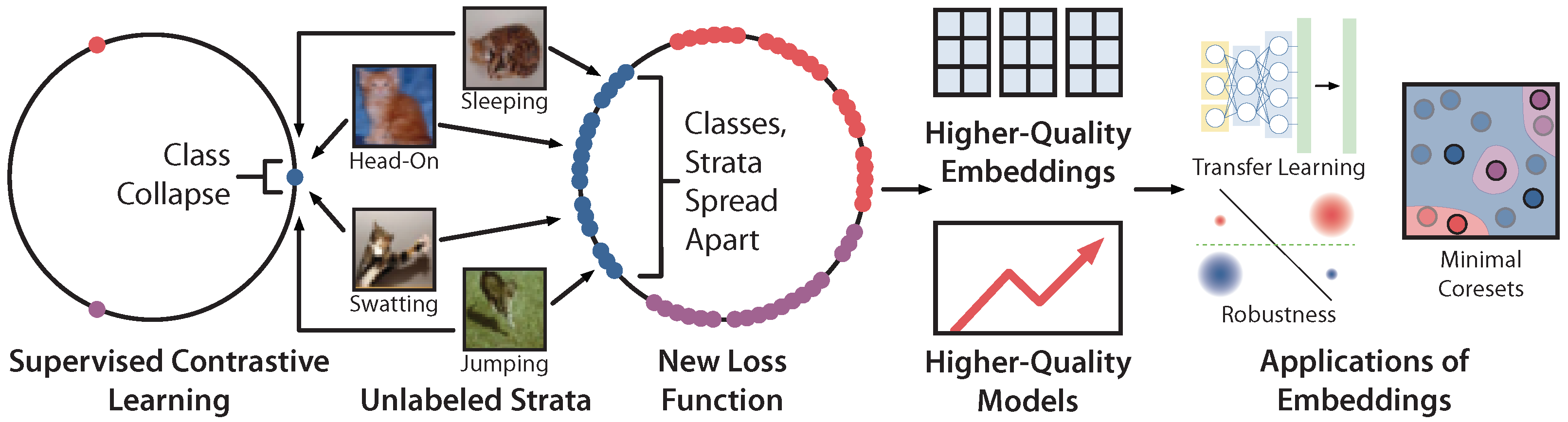
1. Introduction

Supervised contrastive learning has emerged as a promising method for training deep models, with strong empirical results over traditional supervised learning [1]. Recent theoretical work has shown that under certain assumptions, class collapse—when the representation of every point from a class collapses to the same embedding on the hypersphere, as in Figure 1—minimizes the supervised contrastive loss $L_{SC}$ [2]. Furthermore, modern deep networks, which can memorize arbitrary labels [3], are powerful enough to produce class collapse.

Figure 1. Classes contain critical information that is not explicitly encoded in the class labels. Supervised contrastive learning (left) loses this information, since it maps unlabeled strata such as sleeping cats, jumping cats, and swatting cat to a single embedding. We introduce a new loss function $L_{spread}$ that prevents class collapse and maintains strata distinctions. $L_{spread}$ produces higher-quality embeddings, which we evaluate with three downstream applications.

Although class collapse minimizes $L_{SC}$ and produces accurate models, it loses information that is not explicitly encoded in the class labels. For example, consider images with the label “cat.” As shown in Figure 1, some cats may be sleeping, some may be jumping, and some may be swatting at a bug. We call each of these semantically-unique categories of data—some of which are rarer than others, and none of which are explicitly labeled—a stratum. Distinguishing strata is important; it empirically can improve model performance [4] and fine-grained robustness [5]. It is also critical in high-stakes applications such as medical imaging [6]. However, $L_{SC}$ maps the sleeping, jumping, and swatting cats all to a single “cat” embedding, losing strata information. As a result, these embeddings are less useful for common downstream applications in the modern machine learning landscape, such as transfer learning.

In this paper, we explore a simple modification to $L_{SC}$ that prevents class collapse. We study how this modification affects embedding quality by considering how strata are represented in embedding space. We evaluate our loss both in terms of embedding quality, which we evaluate through three downstream applications, and end model quality.

In Section 3, we present our modification to $L_{SC}$, which prevents class collapse by changing how embeddings are pushed and pulled apart. $L_{SC}$ pushes together embeddings of points from the same class and pulls apart embeddings of points from different classes. In contrast, our modified loss $L_{spread}$ includes an additional class-conditional InfoNCE loss term that uniformly pulls apart individual points from within the same class. This term on its own encourages points from the same class to be maximally spread apart in embedding space, which discourages class collapse (see Figure 1 middle). Even though $L_{spread}$ does not use strata labels, we observe that it still produces embeddings that qualitatively appear to retain more strata information than those produced by $L_{SC}$ (see Figure 2).

Figure 2. $L_{spread}$ produces embeddings that are qualitatively better than those produced by $L_{SC}$. We show t-SNE visualizations of embeddings for the CIFAR10 test set and report cosine similarity metrics (average intracluster cosine similarities, and similarities between individual points and the class cluster). $L_{spread}$ produces lower intraclass cosine similarity and embeds images from rare strata further out over the hypersphere than $L_{SC}$.

In Section 4, motivated by these empirical observations, we study how well $L_{spread}$ preserves distinctions between strata in the representation space. Previous theoretical tools that study the optimal embedding distribution fail to characterize the geometry of strata. Instead, we propose a simple thought experiment considering the embeddings that the supervised contrastive loss generates when it is trained on a partial sample of the dataset. This setup enables us to distinguish strata based on their sizes by considering how likely it is for them to be represented in the sample (larger strata are more likely to appear in a small sample). In particular, we find that points from rarer and more distinct strata are clustered less tightly than points from common strata, and we show that this clustering property can improve embedding quality and generalization error.

In Section 5, we empirically validate several downstream implications of these insights. First, we demonstrate that $L_{spread}$ produces embeddings that retain more information about strata, resulting in lift on three downstream applications that require strata recovery:

• We evaluate how well $L_{spread}$’s embeddings encode fine-grained subclasses with coarse-to-fine transfer learning. $L_{spread}$ achieves up to 4.4 points of lift across four datasets.
• We evaluate how well embeddings produced by $L_{spread}$ can recover strata in an unsupervised setting by evaluating robustness against worst-group accuracy and noisy labels. We use our insights about how $L_{spread}$ embeds strata of different sizes to improve worst-group robustness by up to 2.5 points and to recover 75% performance when 20% of the labels are noisy.
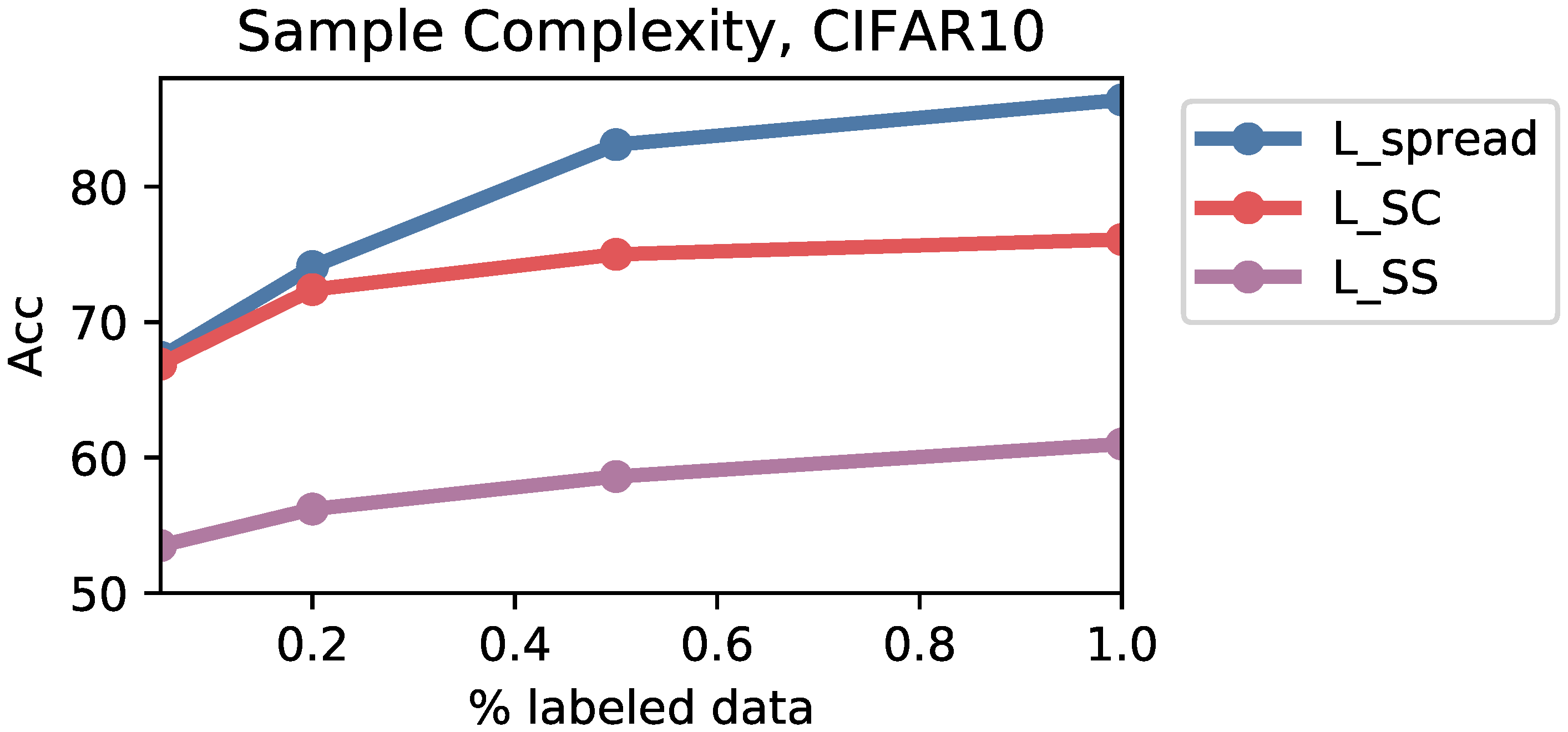
• We evaluate how well we can differentiate rare strata from common strata by constructing limited subsets of the training data that can achieve the highest performance under a fixed training strategy (the coreset problem). We construct coresets by subsampling points from common strata. Our coresets outperform prior work by 1.0 points when coreset size is 30% of the training set.

Next, we find that $L_{spread}$ produces higher-quality models, outperforming $L_{SC}$ by up to 4.0 points across 9 tasks. Finally, we discuss related work in Section 6 and conclude in Section 7.

2. Background

We present our generative model for strata (Section 2.1). Then, we discuss supervised contrastive learning—in particular the SupCon loss $L_{SC}$ from [1] and its optimal embedding distribution [2]—and the end model for classification (Section 2.2).

2.1. Data Setup

We have a labeled input dataset $\mathcal{D}={\left\{(x_i,y_i)\right\}}_{i=1}^N$, where $(x,y)\sim \mathcal{P}$ for $x\in \mathcal{X}$ and $y\in \mathcal{Y}=\{1,\cdots ,K\}$. For a particular data point x, we denote its label as $h\left(x\right)\in \mathcal{Y}$ with distribution $p\left(y\right|x)$. We assume that data is class-balanced such that $p(y=i)=\frac{1}{K}$ for all $i\in \mathcal{Y}$. The goal is to learn a model $\left(y\right|x)$ on $\mathcal{D}$ to classify points.

Data points also belong to categories beyond their labels, called strata. Following [5], we denote a stratum as a latent variable z, which can take on values in $\mathcal{Z}=\{1,\cdots ,C\}$. $\mathcal{Z}$ can be partitioned into disjoint subsets $S_1,\cdots ,S_K$ such that if $z\in S_k$, then its corresponding y label is equal to k. Let $S\left(c\right)$ denote the deterministic label corresponding to stratum c. We model the data generating process as follows. First, the latent stratum is sampled from distribution $p\left(z\right)$. Then, the data point x is sampled from the distribution ${\mathcal{P}}_z=p(·|z)$, and its corresponding label is $y=S\left(z\right)$ (see Figure 2 of [5]). We assume that each class has m strata, and that there exist at least two strata, $z_1,z_2$, where $S\left(z_1\right)\ne S\left(z_2\right)$ and $\mathrm{supp}\left(z_1\right)\cap \mathrm{supp}\left(z_2\right)\ne \varnothing$.

2.2. Supervised Contrastive Loss

Supervised contrastive loss pushes together pairs of points from the same class (called positives) and pulls apart pairs of points from different classes (called negatives) to train an encoder $f:\mathcal{X}\to {\mathbb{R}}^d$. Following previous works, we make three assumptions on the encoder: (1) we restrict the encoder output space to be ${\mathbb{S}}^{d-1}$, the unit hypersphere; (2) we assume $K\le d+1$, which allows Graf et al. [2] to recover optimal embedding geometry; and (3) we assume the encoder f is “infinitely powerful”, meaning that any distribution on ${\mathbb{S}}^{d-1}$ is realizable by $f\left(x\right)$.

2.2.1. SupCon and Collapsed Embeddings

We focus on the SupCon loss $L_{SC}$ from [1]. Denote $\sigma (x,x^{\prime })=f{\left(x\right)}^{\top }f\left(x^{\prime }\right)/\tau$, where $\tau$ is a temperature hyperparameter. Let $\mathcal{B}$ be the set of batches of labeled data on $\mathcal{D}$ and $P(i,B)=\{p\in B\backslash i:h(p)=h(i\left)\right\}$ be the points in B with the same label as $x_i$. For an anchor $x_i$, the SupCon loss is ${\widehat{L}}_{SC}(f,x_i,B)=\frac{-1}{\left|P\right(i,B\left)\right|}{\sum }_{p\in P(i,B)}log\frac{exp\left(\sigma (x_i,x_p)\right)}{{\sum }_{a\in B\backslash i}exp\left(\sigma (x_i,x_a)\right)}$, where $P(i,B)$ forms positive pairs and $B\backslash i$ forms negative pairs.

The optimal embedding distribution that minimizes $L_{SC}$ has one embedding per class, with the per-class embeddings collectively forming a regular simplex inscribed in the hypersphere Graf et al. [2]. Formally, if $h\left(x\right)=i$, then $f\left(x\right)=v_i$ for all $x\in \mathcal{B}$. ${\left\{v_i\right\}}_{i=1}^K$ makes up the regular simplex, defined by: (a) ${\sum }_{i=1}^K{v}_i=0$; (b) $\parallel v_i{\parallel }_2=1$; and (c) $\exists c_K\in \mathbb{R}$ s.t. $v_i^{\top }{v}_j=c_K$ for $i\ne j$. We describe this property as class collapse and define the distribution of $f\left(x\right)$ that satisfies these conditions as collapsed embeddings.

2.2.2. End Model

After the supervised contrastive loss is used to train an encoder, a linear classifier $W\in {\mathbb{R}}^{K\times d}$ is trained on top of the representations $f\left(x\right)$ by minimizing cross-entropy loss over softmax scores. We assume that $\parallel W_y{\parallel }_2\le 1$ for each $y\in \mathcal{Y}$. The end model’s empirical loss can be defined as $\widehat{\mathcal{L}}(W,\mathcal{D})={\sum }_{x_i\in \mathcal{D}}-log\frac{exp\left(f{\left(x_i\right)}^{\top }{W}_{h\left(x_i\right)}\right)}{{\sum }_{j=1}^{K}exp\left(f{\left(x_i\right)}^{\top }{W}_j\right)}$. The model uses softmax scores constructed with $f\left(x\right)$ and W to generate predictions $\widehat{p}\left(y\right|x)$, which we also write as $\widehat{p}\left(y\right|f\left(x\right))$. Finally, the generalization error of the model on $\mathcal{P}$ is the expected cross-entropy between $\widehat{L}\left(y\right|x)$ and $p\left(y\right|x)$, namely $\mathcal{L}(x,y,f)={\mathbb{E}}_{x,y\sim \mathcal{P}}\left[-log\left(y\right|f\left(x\right))\right]$.

3. Method

We now highlight some theoretical problems with class collapse under our generative model of strata (Section 3.1). We then propose and qualitatively analyze the loss function $L_{spread}$ (Section 3.2).

3.1. Theoretical Motivation

We show that the conditions under which collapsed embeddings minimize generalization error on coarse-to-fine transfer and the original task do not hold when distinct strata exist.

Consider the downstream coarse-to-fine transfer task $(x,z)$ of using embeddings $f\left(x\right)$ learned on $(x,y)$ to classify points by fine-grained strata. Formally, coarse-to-fine transfer involves learning an end model with weight matrix $W\in {\mathbb{R}}^{C\times d}$ and fixed $f\left(x\right)$ (as described in Section 2.2) on points $(x,z)$, where we assume the data are class-balanced across z.

Observation 1.

Class collapse minimizes $\mathcal{L}(x,z,f)$ if for all x, (1) $p(y=h(x\left)\right|x)=1$, meaning that each x is deterministically assigned to one class, and (2) $p\left(z\right|x)=\frac{1}{m}$ where $z\in S_{h\left(x\right)}$. The second condition implies that $p\left(x\right|z)=p(x\left|y\right)$ for all $z\in S_y$, meaning that there is no distinction among strata from the same class. This contradicts our data model described in Section 2.1.

Similarly, we characterize when collapsed embeddings are optimal for the original task $(x,y)$.

Observation 2.

Class collapse minimizes $\mathcal{L}(x,y,f)$ if, for all x, $p(y=h(x\left)\right|x)=1$. This contradicts our data model.

Proofs are in Appendix D.1. We also analyze transferability of f on arbitrary new distributions $(x^{\prime },y^{\prime })$ information-theoretically in Appendix C.1, finding that a one-to-one encoder obeys the Infomax principle [7] better than collapsed embeddings on $(x^{\prime },y^{\prime })$. These observations suggest that a distribution over the embeddings that preserves strata distinctions and does not collapse classes is more desirable.

3.2. Modified Contrastive Loss $L_{spread}$

We introduce the loss $L_{spread}$, a weighted sum of two contrastive losses $L_{attract}$ and $L_{repel}$. $L_{attract}$ is a supervised contrastive loss, while $L_{repel}$ encourages intra-class separation. For $\alpha \in [0,1]$,

$$\begin{array}{cc}\hfill L_{spread}& =\alpha L_{attract}+(1-\alpha )L_{repel}.\hfill \end{array}$$

(1)

For a given anchor $x_i$, define $x_i^{aug}$ as an augmentation of the same point as x. Define the set of negative examples for i to be $N(i,B)=\{a\in B\backslash i:h(a)\ne h(i\left)\right\}$. Then,

$$\begin{array}{cc}\hfill {\widehat{L}}_{attract}(f,x_i,B)& =\frac{-1}{\left|P\right(i,B\left)\right|}\times \sum _{p\in P(i,B)}log\frac{exp\left(\sigma (x_i,x_p)\right)}{exp\left(\sigma (x_i,x_p)\right)+{\sum }_{a\in N(i,B)}exp\left(\sigma (x_i,x_a)\right)}\hfill \end{array}$$

(2)

$$\begin{array}{cc}\hfill {\widehat{L}}_{repel}(f,x_i,B)& =-log\frac{exp\left(\sigma (x_i,x_i^{aug})\right)}{{\sum }_{p\in P(i,B)}exp\left(\sigma (x_i,x_p)\right)}.\hfill \end{array}$$

(3)

${\widehat{L}}_{attract}$ is a variant of the SupCon loss, which encourages class separation in embedding space as suggested by Graf et al. [2]. ${\widehat{L}}_{repel}$ is a class-conditional InfoNCE loss, where the positive distribution consists of augmentations and the negative distribution consists of i.i.d samples from the same class. It encourages points within a class to be spread apart, as suggested by the analysis of the InfoNCE loss by Wang and Isola [8].

Qualitative Evaluation

Figure 2 shows t-SNE plots for embeddings produced with $L_{SC}$ versus $L_{spread}$ on the CIFAR10 test set. $L_{spread}$ produces embeddings that are more spread out than those produced by $L_{SC}$ and avoids class collapse. As a result, images from different strata can be better differentiated in embedding space. For example, we show two dogs, one from a common stratum and one from a rare stratum (rare pose). The two dogs are much more distinguishable by distance in the $L_{spread}$ embedding space, which suggests that it helps preserve distinctions between strata.

4. Geometry of Strata

We first discuss some existing theoretical tools for analyzing contrastive loss geometrically and their shortcomings with respect to understanding how strata are embedded. In Section 4.2, we propose a simple thought experiment about the distances between strata in embedding space when trained under a finite subsample of data to better understand our prior qualitative observations. Then, in Section 4.3, we discuss implications of representations that preserve strata distinctions, showing theoretically how they can yield better generalization error on both coarse-to-fine transfer and the original task and empirically how they allow for new downstream applications.

4.1. Existing Analysis

Previous works have studied the geometry of optimal embeddings under contrastive learning [2,8,9], but their techniques cannot analyze strata because strata information is not directly used in the loss function. These works use the infinite encoder assumption, where any distribution on ${\mathbb{S}}^{d-1}$ is realizable by the encoder f applied to the input data. This allows the minimization of the contrastive loss to be equivalent to an optimization problem over probability measures on the hypersphere. As a result, solving this new problem yields a distribution whose characterization is solely determined by information in the loss function (e.g., labels information [2,9]) and is decoupled from other information about the input data x and hence decoupled from strata.

More precisely, if we denote the measure of $x\in \mathcal{X}$ as ${\mu }_{\mathcal{X}}$, minimizing the contrastive loss over the mapping f is equal (at the population level) to minimizing over the pushforward measure ${\mu }_{\mathcal{X}}\circ f^{-1}:{\mathbb{S}}^{d-1}\to [0,1]$. The infinite encoder assumption allows us to relax the problem and instead consider optimizing over any $\mu \in \mathcal{M}\left({\mathbb{S}}^{d-1}\right)$ in the Borel set of probability measures on the hypersphere. Then, the optimal ${\mu }^{★}$ learned is independent of the distribution of the input data $\mathcal{P}$ beyond what is in the relaxed objective function.

This approach using the infinite encoder assumption does not allow for analysis of strata. Strata are unknown at training time and thus cannot be incorporated explicitly into the loss function. Their geometries will not be reflected in the characterization of the optimal distribution obtained from previous theoretical tools. Therefore, we need additional reasoning for our empirical observations that strata distinctions are preserved in embedding space under $L_{spread}$.

4.2. Subsampling Strata

We propose a simple thought experiment based on subsampling the dataset—randomly sampling a fraction of the training data—to analyze strata. Consider the following: we subsample a fraction $t\in [0,1]$ of a training set of N points from $\mathcal{P}$. We use this subsampled dataset ${\mathcal{D}}_t$ to learn an encoder ${\widehat{f}}_t$, and we study the average distance under ${\widehat{f}}_t$ between two strata z and $z^{\prime }$ as t varies.

The average distance between z and $z^{\prime }$ is $\delta ({\widehat{f}}_t,z,z^{\prime })={\parallel {\mathbb{E}}_{x\sim {\mathcal{P}}_z}\left[{\widehat{f}}_t\left(x\right)\right]-{\mathbb{E}}_{x\sim {\mathcal{P}}_{z^{\prime }}}\left[{\widehat{f}}_t\left(x\right)\right]\parallel }_2$ and depends on whether z and $z^{\prime }$ are both in the subsampled dataset. We study when z and $z^{\prime }$ belong to the same class. We have three cases (with probabilities stated in Appendix C.2) based on strata frequency and t—when both, one, or neither of the strata appears in ${\mathcal{D}}_t$:

• Both strata appear in ${\mathcal{D}}_t$ The encoder ${\widehat{f}}_t$ is trained on both z and $z^{\prime }$. For large N, we can approximate this setting by considering ${\widehat{f}}_t$ trained on infinite data from these strata. Points belonging to these strata will be defined in the optimal embedding distribution on the hypersphere, which can be characterized by prior theoretical approaches [2,8,9]. With $L_{spread}$, $\delta ({\widehat{f}}_t,z,z^{\prime })$ depends on $\alpha$, which controls the extent of spread in the embedding geometry. With $L_{SC}$, points from the two strata would asymptotically map to one location on the hypersphere, and $\delta ({\widehat{f}}_t,z,z^{\prime })$ would converge to 0. This case occurs with probability increasing in $p\left(z\right),p\left(z^{\prime }\right),$ and t.
• One stratum but not the other appears in ${\mathcal{D}}_t$ Without loss of generality, suppose that points from z appear in ${\mathcal{D}}_t$ but no points from $z^{\prime }$ do. To understand $\delta ({\widehat{f}}_t,z,z^{\prime })$, we can consider how the end model $\widehat{p}\left(y\right|{\widehat{f}}_t\left(x\right))$ learned using the “source” distribution containing z performs on the “target” distribution of stratum $z^{\prime }$ since this downstream classifier is a function of distances in embedding space. Borrowing from the literature in domain adaptation, the difficulty of this out-of-distribution problem depends on both the divergence between source z and target $z^{\prime }$ distributions and the capacity of the overall model. The $\mathcal{H}\Delta \mathcal{H}$-divergence from Ben-David et al. [10,11], which is studied in lower bounds in Ben-David and Urner [12], and the discrepancy difference from Mansour et al. [13] capture both concepts. Moreover, the optimal geometries of $L_{spread}$ and $L_{SC}$ induce different end model capacities and prediction distributions, with data being more separable under $L_{SC}$, which can help explain why $L_{spread}$ better preserves strata distances. This case occurs with probability increasing in $p\left(z\right)$ and decreasing in $p\left(z^{\prime }\right)$ and t.
• Neither strata appears in ${\mathcal{D}}_t$ The distance $\delta ({\widehat{f}}_t,z,z^{\prime })$ in this case is at most $2D_{\mathrm{TV}}({\mathcal{P}}_z,{\mathcal{P}}_{z^{\prime }})$ (total variation distance) regardless of how the encoder is trained, although differences in transfer from models learned on $\mathcal{Z}\backslash z,z^{\prime }$ to z versus $z^{\prime }$ can be further analyzed. This case occurs with probability decreasing in $p\left(z\right),p\left(z^{\prime }\right),$ and t.

We make two observations from these cases. First, if z and $z^{\prime }$ are both common strata, then as t increases, the distance between them depends on the optimal asymptotic distribution. Therefore, if we set $\alpha =1$ in $L_{spread}$, these common strata will collapse. Second, if z is a common strata and $z^{\prime }$ is uncommon, the second case occurs frequently over randomly sampled ${\mathcal{D}}_t$, and thus the strata are separated based on the difficulty of the respective out-of-distribution problem. We thus arrive at the following insight from our thought experiment:

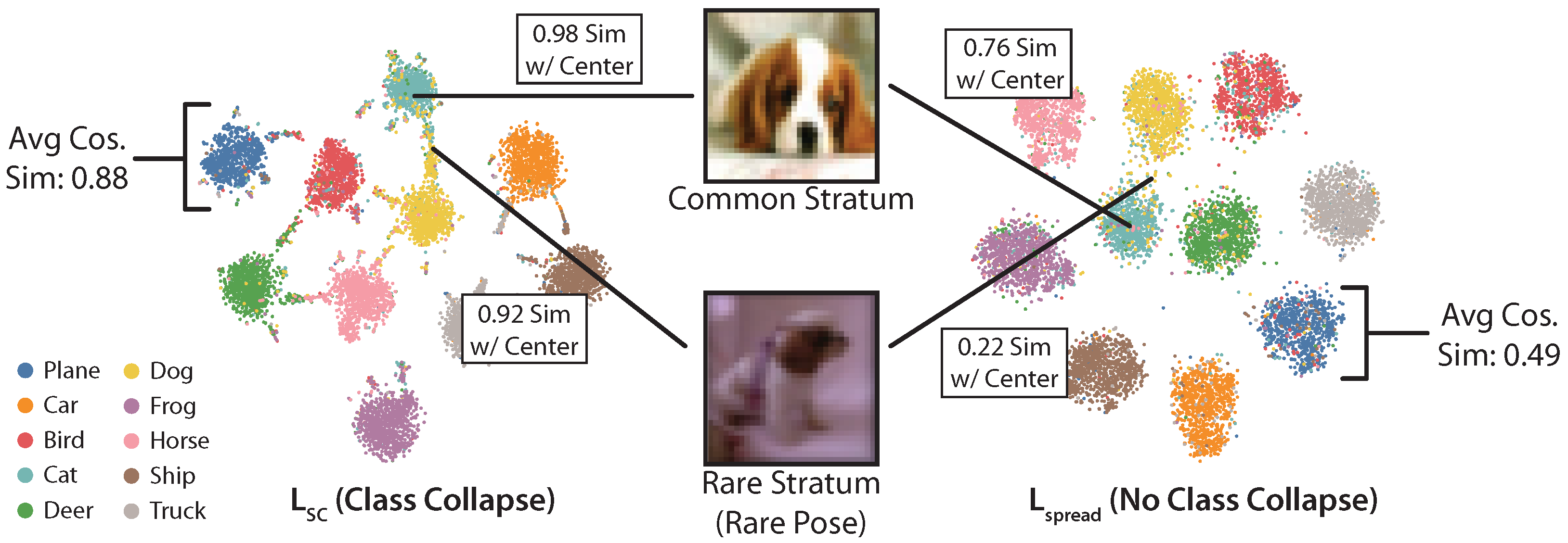
Common strata are more tightly clustered together, while rarer and more semantically distinct strata are far away from them.

Figure 3 demonstrates this insight. It shows a t-SNE visualization of embeddings from training on CIFAR100 with coarse superclass labels, and with artifically imbalanced subclasses. We show points from the largest subclasses in dark blue and points from the smallest subclasses in light blue. Points from the largest subclasses (dark blue) cluster tightly, whereas points from small subclasses (light blue) are scattered throughout the embedding space.

Figure 3. Points from large subclasses cluster tightly; points from small subclasses scatter (CIFAR100-Coarse, unbalanced subclasses).

4.3. Implications

We discuss theoretical and practical implications of our subsampling argument. First, we show that on both the coarse-to-fine transfer task $(x,z)$ and the original task $(x,y)$, embeddings that preserve strata yield better generalization error. Second, we discuss practical implications arising from our subsampling argument that enable new applications.

4.3.1. Theoretical Implications

Consider ${\widehat{f}}_1$, the encoder trained on $\mathcal{D}$ with all N points using $L_{spread}$, and suppose a mean classifier is used for the end model, e.g., $W_y={\mathbb{E}}_{x|y}\left[{\widehat{f}}_1\left(x\right)\right]$ and $W_z={\mathbb{E}}_{x|z}\left[{\widehat{f}}_1\left(x\right)\right]$. On coarse-to-fine transfer, generalization error depends on how far each stratum center is from the others.

Lemma 1.

There exists ${\lambda }_z>0$ such that the generalization error on the coarse-to-fine transfer task is at most

$$\begin{array}{c}\hfill \mathcal{L}(x,z,{\widehat{f}}_1)\le {\mathbb{E}}_z\left[log\left(\sum _{z^{\prime }\in \mathcal{Z}}exp\left(-{\lambda }_z\left(\frac{1}{2}\delta {({\widehat{f}}_1,z,z^{\prime })}^2-1\right)\right)\right)\right]-1,\end{array}$$

(4)

where $\delta ({\widehat{f}}_1,z,z^{\prime })$ is the average distance between strata z and $z^{\prime }$ defined in Section 4.2.

The larger the distances between strata, the smaller the upper bound on generalization error. We now show that a similar result holds on the original task $(x,y)$, but there is an additional term that penalizes points from the same class being too far apart.

Lemma 2.

There exists ${\lambda }_y>0$ such that the generalization error on the original task is at most

$$\begin{array}{cc}\hfill \mathcal{L}(x,y,{\widehat{f}}_1)\le {\mathbb{E}}_z[& {\mathbb{E}}_{z^{\prime }|S\left(z\right)}\left[\frac{1}{2}\delta {({\widehat{f}}_1,z,z^{\prime })}^2-1\right]\hfill \end{array}$$

(5)

$$\begin{array}{cc}\hfill & +log\left(\sum _{y\in \mathcal{Y}}exp\left({\mathbb{E}}_{z^{\prime }|y}\left[-{\lambda }_y\left(\frac{1}{2}\delta {({\widehat{f}}_1,z,z^{\prime })}^2-1\right)\right]\right)\right)].\hfill \end{array}$$

(6)

This result suggests that maximizing distances between strata of different classes is desirable, but less so for distances between strata of the same class as suggested by the first term in the expression. Both results illustrate that separating strata to some extent in the embedding space results in better bounds on generalization error. In Appendix C.3, we provide proofs of these results and derive values of the generalization error for these two tasks under class collapse for comparison.

4.3.2. Practical Implications

Our discussion in Section 4.2 suggests that training with $L_{spread}$ better distinguishes strata in embedding space. As a result, we can use differences between strata of different sizes for downstream applications. For example, unsupervised clustering can help recover pseudolabels for unlabeled, rare strata. These pseudolabels can be used as inputs to worst-group robustness algorithms, or used to detect noisy labels, which appear to be rare strata during training (see Section 5.3 for examples). We can also train over subsampled datasets to heuristically distinguish points that come from common strata from points that come from rare strata. We can then downsample points from common strata to construct minimal coresets (see Section 5.4 for examples).

5. Experiments

This section evaluates $L_{spread}$ on embedding quality and model quality:

• First, in Section 5.2, we use coarse-to-fine transfer learning to evaluate how well the embeddings maintain strata information. We find that $L_{spread}$ achieves lift across four datasets.
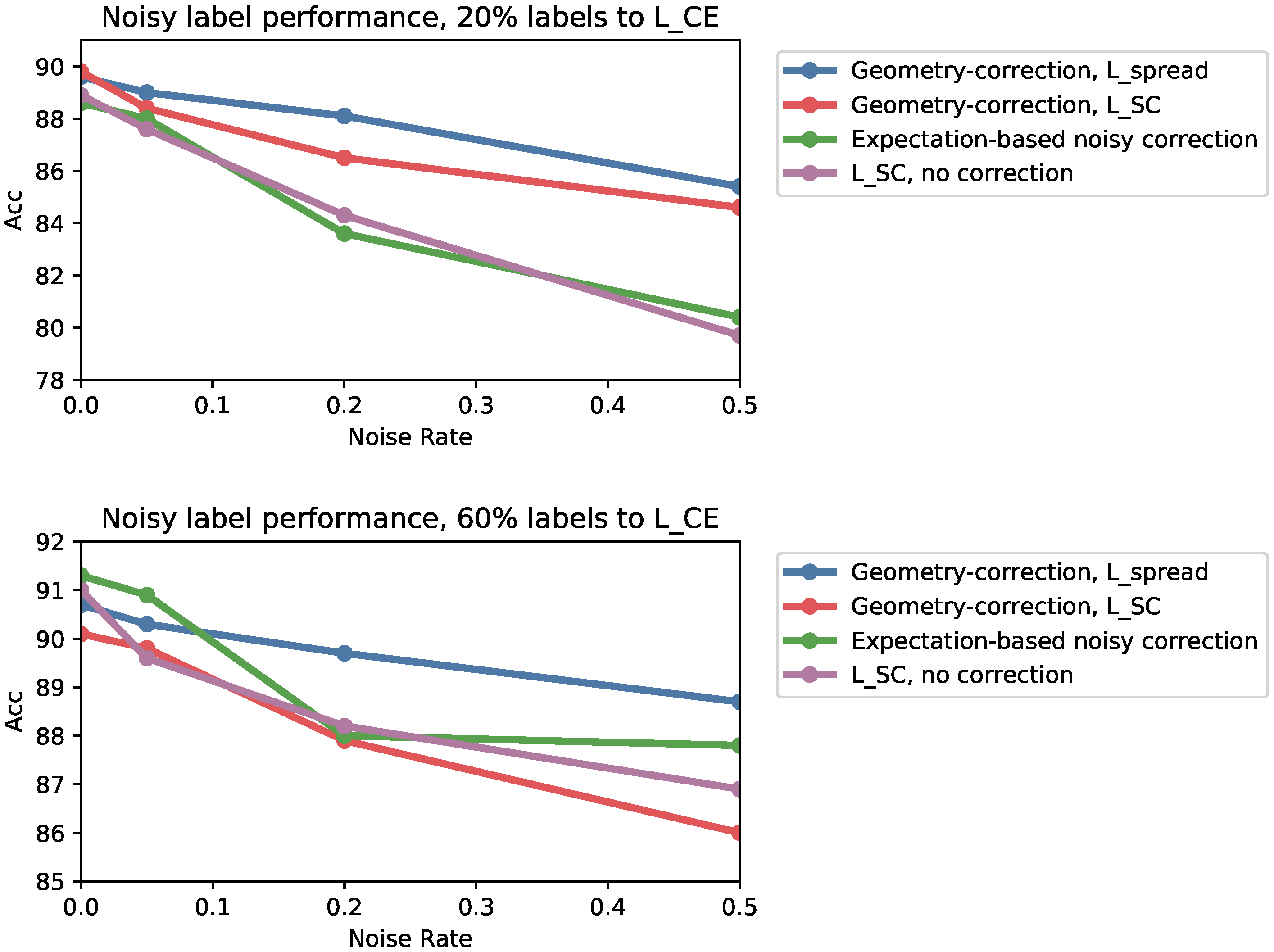
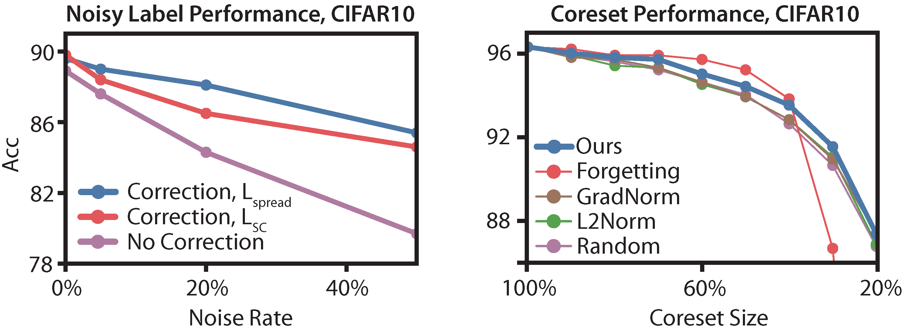
• In Section 5.3, we evaluate how well $L_{spread}$ can detect rare strata in an unsupervised setting. We first use $L_{spread}$ to detect rare strata to improve worst-group robustness by up to 2.5 points. We then use rare strata detection to correct noisy labels, recovering 75% performance under 20% noise.
• In Section 5.4, we evaluate how well $L_{spread}$ can distinguish points from large strata versus points from small strata. We downsample points from large strata to construct minimal coresets on CIFAR10, outperforming prior work by 1.0 points at 30% labeled data.
• Finally, in Section 5.5, we show that training with $L_{spread}$ improves model quality, validating our theoretical claims that preventing class collapse can improve generalization error. We find that $L_{spread}$ improves performance in 7 out of 9 cases.

5.1. Datasets and Models

Tabel Table 1 lists all the datasets we use in our evaluation. CIFAR10, CIFAR100, and MNIST are the standard computer vision datasets. We also use coarse versions of each, wherein classes are combined to create coarse superclasses (animals/vehicles for CIFAR10, standard superclasses for CIFAR100, and <5, ≥5 for MNIST). In CIFAR100-Coarse-U, some subclasses have been artificially imbalanced. Waterbirds, ISIC and CelebA are image datasets with documented hidden strata [5,14,15,16]. We use a ViT model [17] (4 × 4, 7 layers) for CIFAR and MNIST and a ResNet50 for the rest. For the ViT models, we jointly optimize the contrastive loss with a cross entropy loss head. For the ResNets, we train the contrastive loss on its own and use linear probing on the final layer. More details in Appendix E.

Table 1. Summary of the datasets we use for evaluation.

Dataset	Notes
CIFAR10	Standard computer vision dataset
CIFAR10-Coarse	CIFAR10 with animal/vehicle coarse labels
CIFAR100	Standard computer vision dataset
CIFAR100-Coarse	CIFAR100 with standard coarse labels
CIFAR100-Coarse-U	CIFAR100 with standard coarse labels, but with some fine classes
	sub-sampled
MNIST	Standard computer vision dataset
MNIST-Coarse	MNIST with <5 and ≥5 coarse labels
Waterbirds	Robustness dataset mixing up images of birds and their
	backgrounds [14]
ISIC	Images of skin lesions [15]
CelebA	Images of celebrity faces [16]

5.2. Coarse-to-Fine Transfer Learning

In this section, we use coarse-to-fine transfer learning to evaluate how well $L_{spread}$ retains strata information in the embedding space. We train on coarse superclass labels, freeze the weights, and then use transfer learning to train a linear layer with subclass labels. We use this supervised strata recovery setting to isolate how well the embeddings can recover strata in the optimal setting. For baselines, we compare against training with $L_{SC}$ and the SimCLR loss $L_{SS}$.

Table 2 reports the results. We find that $L_{spread}$ produces better embeddings for coarse-to-fine transfer learning than $L_{SC}$ and $L_{SS}$. Lift over $L_{SC}$ varies from 0.2 points on MNIST (16.7% error reduction), to 23.6 points of lift on CIFAR10. $L_{spread}$ also produces better embeddings than $L_{SS}$, since $L_{SS}$ does not encode superclass labels in the embedding space.

Table 2. Performance of coarse-to-fine transfer on various datasets compared against contrastive baselines. In these tasks, we first train a model on coarse task labels, then freeze the representation and train a model on fine-grained subclass labels. $L_{spread}$ produces embeddings that transfer better across all datasets. Best in bold.

	Coarse-to-Fine Transfer
Dataset	${\mathit{L}}_{\mathbf{SS}}$	${\mathit{L}}_{\mathbf{SC}}$	${\mathit{L}}_{\mathbf{spread}}$
CIFAR10-Coarse	71.7	52.5	76.1
CIFAR100-Coarse	62.0	62.4	63.9
CIFAR100-Coarse-U	61.9	59.5	62.4
MNIST-Coarse	97.1	98.8	99.0

5.3. Robustness against Worst-Group Accuracy and Noise

In this section, we use robustness to measure how well $L_{spread}$ can recover strata in an unsupervised setting. We use clustering to detect rare strata as an input to worst-group robustness algorithms, and we use a geometric heuristic over embeddings to correct noisy labels.

To evaluate worst-group accuracy, we follow the experimental setup and datasets from Sohoni et al. [5]. We first train a model with class labels. We then cluster the embeddings to produce pseudolabels for hidden strata, which we use as input for a Group-DRO algorithm to optimize worst-group robustness [14]. We use both $L_{SC}$ and cross entropy loss [5] for training the first stage as baselines.

To evaluate robustness against noise, we introduce noisy labels to the contrastive loss head on CIFAR10. We detect noisy labels with a simple geometric heuristic: points with incorrect labels appear to be small strata, so they should be far away from other points of the same class. We then correct noisy points by assigning the label of the nearest cluster in the batch. More details can be found in Appendix E.

Table 3 shows the performance of unsupervised strata recovery and downstream worst-group robustness. We can see that $L_{spread}$ outperforms both $L_{SC}$ and Sohoni et al. [5] on strata recovery. This translates to better worst-group robustness on Waterbirds and CelebA.

Table 3. Unsupervised strata recovery performance (top, F1), and worst-group performance (AUROC for ISIC, Acc for others) using recovered strata. Best in bold.

	Sub-Group Recovery
Dataset	Sohoni et al. [5]	${\mathit{L}}_{\mathbf{SC}}$	${\mathit{L}}_{\mathbf{spread}}$
Waterbirds	56.3	47.2	59.0
ISIC	74.0	92.5	93.8
CelebA	24.2	19.4	24.8
	Worst-Group Robustness
Waterbirds	88.4	86.5	89.0
ISIC	92.0	93.3	92.6
CelebA	55.0	66.1	67.8

Figure 4 (left) shows the effect of noisy labels on performance. When noisy labels are uncorrected (purple), performance drops by up to 10 points at 50% noise. Applying our geometric heuristic (red) can recover 4.8 points at 50% noise, even without using $L_{spread}$. However, $L_{spread}$ recovers an additional 0.9 points at 50% noise, and an additional 1.6 points at 20% noise (blue). In total, $L_{spread}$ recovers 75% performance at 20% noise, whereas $L_{SC}$ only recovers 45% performance.

Figure 4. (Left) Performance of models under various amounts of label noise for the contrastive loss head. (Right) Performance of a ResNet18 trained with coresets of various sizes. Our coreset algorithm is competitive with the state-of-the-art in the large coreset regime (from 40–90% coresets), but maintains performance for small coresets (smaller than 40%). At the 10% coreset, our algorithm outperforms [18] by 32 points and matches random sampling.

5.4. Minimal Coreset Construction

Now we evaluate how well training on fractional samples of the dataset with $L_{spread}$ can distinguish points from large versus small strata by constructing minimal coresets for CIFAR10. We train a ResNet18 on CIFAR10, following Toneva et al. [18], and compare against baselines from Toneva et al. [18] (Forgetting) and Paul et al. [19] (GradNorm, L2Norm). For our coresets, we train with $L_{spread}$ on subsamples of the dataset and record how often points are correctly classified at the end of each run. We bucket points in the training set by how often the point is correctly classified. We then iteratively remove points from the largest bucket in each class. Our strategy removes easy examples first from the largest coresets, but maintains a set of easy examples in the smallest coresets.

Figure 4 (right) shows the results at various coreset sizes. For large coresets, our algorithm outperforms both methods from Paul et al. [19] and is competitive with Toneva et al. [18]. For small coresets, our method outperforms the baselines, providing up to 5.2 points of lift over Toneva et al. [18] at 30% labeled data. Our analysis helps explain this gap; removing too many easy examples hurts performance, since then the easy examples become rare and hard to classify.

5.5. Model Quality

Finally, we confirm that $L_{spread}$ produces higher-quality models and achieves better sample complexity than both $L_{SC}$ and the SimCLR loss $L_{SS}$ from [20]. Table 4 reports the performance of models across all our datasets. We find that $L_{spread}$ achieves better overall performance compared to models trained with $L_{SC}$ and $L_{SS}$ in 7 out of 9 tasks, and matches performance in 1 task. We find up to 4.0 points of lift over $L_{SC}$ (Waterbirds), and up to 2.2 points of lift (AUROC) over $L_{SS}$ (ISIC). In Appendix F, we additionally evaluate the sample complexity of contrastive losses by training on partial subsamples of CIFAR10. $L_{spread}$ outperforms $L_{SC}$ and $L_{SS}$ throughout.

Table 4. End model performance training with $L_{spread}$ on various datasets compared against contrastive baselines. All metrics are accuracy except for ISIC (AUROC). $L_{spread}$ produces the best performance in 7 out of 9 cases, and matches the best performance in 1 case. Best in bold.

	End Model Perf.
Dataset	${\mathit{L}}_{\mathbf{SS}}$	${\mathit{L}}_{\mathbf{SC}}$	${\mathit{L}}_{\mathbf{spread}}$
CIFAR10	89.7	90.9	91.5
CIFAR10-Coarse	97.7	96.5	98.1
CIFAR100	68.0	67.5	69.1
CIFAR100-Coarse	76.9	77.2	78.3
CIFAR100-Coarse-U	72.1	71.6	72.4
MNIST	99.1	99.3	99.2
MNIST-Coarse	99.1	99.4	99.4
Waterbirds	77.8	73.9	77.9
ISIC	87.8	88.7	90.0

6. Related Work and Discussion

From work in contrastive learning, we take inspiration from [21], who use a latent classes view to study self-supervised contrastive learning. Similarly, [22] considers how minimizing the InfoNCE loss recovers a latent data generating model. We initially started from a debiasing angle to study the effects of noise in supervised contrastive learning inspired by [23], but moved to our current strata-based view of noise instead. Recent work has also analyzed contrastive learning from the information-theoretic perspective [24,25,26], but does not fully explain practical behavior [27], so we focus on the geometric perspective in this paper because of the downstream applications. On the geometric side, we are inspired by the theoretical tools from [8] and [2], who study representations on the hypersphere along with [9].

Our work builds on the recent wave of empirical interest in contrastive learning [20,28,29,30,31] and supervised contrastive learning [1]. There has also been empirical work analyzing the transfer performance of contrastive representations and the role of intra-class variability in transfer learning. [32] find that combining supervised and self-supervised contrastive loss improves transfer learning performance, and they hypothesize that this is due to both inter-class separation and intra-class variability. [33] find that combining cross entropy and self-supervised contrastive loss improves coarse-to-fine transfer, also motivated by preserving intra-class variability.

We derive $L_{spread}$ from similar motivations to losses proposed in these works, and we futher theoretically study why class collapse can hurt downstream performance. In particular, we study why preserving distinctions of strata in embedding space may be important, with theoretical results corroborating their empirical studies. We further propose a new thought experiment for why a combined loss function may lead to better separation of strata.

Our treatment of strata is strongly inspired by [5,6], who document empirical consequences of hidden strata. We are inspired by empirical work that has demonstrated that detecting subclasses can be important for performance [4,34] and robustness [14,35,36].

Each of our downstream applications is a field in itself, and we take inspiration from recent work from each. Our noise heuristic is similar to the ELR [37] and takes inspiration from a various work using contrastive learning to correct noisy labels and for semi-supervised learning [38,39,40]. Our coreset algorithm is inspired by recent work in coresets for modern deep networks [19,41,42], and takes inspiration from [18] in particular.

7. Conclusions

We propose a new supervised contrastive loss function to prevent class collapse and produce higher-quality embeddings. We discuss how our loss function better maintains strata distinctions in embedding space and explore several downstream applications. Future directions include encoding label hierarchies and other forms of knowledge in contrastive loss functions and extending our work to more modalities, models, and applications. We hope that our work inspires further work in more fine-grained supervised contrastive loss functions and new theoretical approaches for reasoning about generalization and strata.

Appendix C.1. Transfer Learning on $(x^{\prime },y^{\prime })$

We now show an additional transfer learning result on new tasks $(x^{\prime },y^{\prime })$. Formally, recall that we learn the encoder f on $(x,y)\sim \mathcal{P}$. We wish to use it on a new task with target distribution $(x^{\prime },y^{\prime })\sim {\mathcal{P}}^{\prime }$. We find that an injective encoder $f\left(x\right)$ is more appropriate to be used on new distributions than collapsed embeddings based on the Infomax principle [7].

Observation A1.

Define $f_c\left(y\right)$ as the mapping to collapsed embeddings and $f_{1-1}\left(x\right)$ as an injective mapping, both learned on $\mathcal{P}$. Construct a new variable $\tilde{y}$ with joint distribution $(x^{\prime },\tilde{y})\sim p\left(y\right|x)·p^{\prime }\left(x^{\prime }\right)$ and suppose that $\tilde{y}⫫y^{\prime }|x^{\prime }$. Then, by the data processing inequality, it holds that $I(\tilde{y},y^{\prime })\le I(x^{\prime },y^{\prime })$ where $I(·,·)$ is the mutual information between two random variables. We apply $f_c$ to $\tilde{y}$ and $f_{1-1}$ to $x^{\prime }$ to get that

$$\begin{array}{c}\hfill I(f_c\left(\tilde{y}\right),y^{\prime })\le I(f_{1-1}\left(x^{\prime }\right),y^{\prime }).\end{array}$$

Therefore, $f_{1-1}$ obeys the Infomax principle [7] better on ${\mathcal{P}}^{\prime }$ than $f_c$. Via Fano’s inequality, this statement implies that the Bayes risk for learning $y^{\prime }$ from $x^{\prime }$ is lower using $f_{1-1}$ than $f_c$.

Appendix C.2. Probabilities of Strata $z,z^{\prime }$ Appearing in Subsampled Dataset

As discussed in Section 4.2, the distance between strata z and $z^{\prime }$ in embedding space depends on if these strata appear in the subsampled dataset ${\mathcal{D}}_t$ that the encoder was trained on. We define the exact probabilities of the three cases presented. Let $Pr(z,z^{\prime }\in {\mathcal{D}}_t)$ be the probability that both strata are seen, $Pr(z\in {\mathcal{D}}_t,z^{\prime }\notin {\mathcal{D}}_t)$ be the probability that only z is seen, and $Pr(z,z^{\prime }\notin {\mathcal{D}}_t)$ be the probability that neither are seen.

First, the probability of neither strata appearing in ${\mathcal{D}}_t$ is easy to compute. In particular, we have that $Pr(z,z^{\prime }\notin {\mathcal{D}}_t)={(1-p\left(z\right)-p\left(z^{\prime }\right))}^{tN}$. This quantity decreases in $p\left(z\right)$ and $p\left(z^{\prime }\right)$, confirming that it is less likely for two common strata to not appear in ${\mathcal{D}}_t$.

Second, the probability of z being in ${\mathcal{D}}_t$ and $z^{\prime }$ not being in ${\mathcal{D}}_t$ can be expressed as $Pr(z\in {\mathcal{D}}_t|z^{\prime }\notin {\mathcal{D}}_t)·Pr(z^{\prime }\notin {\mathcal{D}}_t)$. $Pr(z^{\prime }\notin {\mathcal{D}}_t)$ is equal to ${(1-p\left(z^{\prime }\right))}^{tN}$, and $Pr(z\in {\mathcal{D}}_t|z^{\prime }\notin {\mathcal{D}}_t)=1-Pr(z\notin {\mathcal{D}}_t|z^{\prime }\notin {\mathcal{D}}_t)=1-(1-p(z|z\in \mathcal{Z}\backslash z^{\prime }{\left)\right)}^{tN}$. Finally, note that $p\left(z\right|z\in \mathcal{Z}\backslash z^{\prime })=\frac{p\left(z\right)}{1-p\left(z^{\prime }\right)}$. Putting this together, we get that $Pr(z\in {\mathcal{D}}_t,z^{\prime }\notin {\mathcal{D}}_t)={(1-p\left(z^{\prime }\right))}^{tN}-{(1-p\left(z^{\prime }\right)-p\left(z\right))}^{tN}$, and we can similarly construct $Pr(z^{\prime }\in {\mathcal{D}}_t,z\notin {\mathcal{D}}_t)$. This quantity depends on the difference between $p\left(z\right)$ and $p\left(z^{\prime }\right)$, so this case is common when one stratum is common and one is rare.

Lastly, the probability of both z and $z^{\prime }$ being in ${\mathcal{D}}_t$ is thus $Pr(z,z^{\prime }\in {\mathcal{D}}_t)=1-Pr(z,z^{\prime }\notin {\mathcal{D}}_t)-Pr(z^{\prime }\in {\mathcal{D}}_t,z\notin {\mathcal{D}}_t)-Pr(z\in {\mathcal{D}}_t,z^{\prime }\notin {\mathcal{D}}_t)=1+{(1-p\left(z^{\prime }\right)-p\left(z\right))}^{tN}-{(1-p\left(z^{\prime }\right))}^{tN}-{(1-p\left(z\right))}^{tN}$. This quantity increases in $p\left(z\right)$ and $p\left(z^{\prime }\right)$.

Appendix C.3. Performance of Collapsed Embeddings on Coarse-to-Fine Transfer and Original Task

Lemma A1.

Denote $f_c$ to be the encoder that collapses embeddings such that $f_c\left(x\right)=v_y$ for any $(x,y)\sim \mathcal{P}$. Then, the generalization error on the coarse-to-fine transfer task using $f_c$ and a linear classifier learned using cross entropy loss is at least

$$\begin{array}{c}\hfill \mathcal{L}(x,z,f_c)\ge log(mexp\left(1\right)+(C-m)exp\left(c_K\right)-1,\end{array}$$

where $c_K$ is the dot product of any two different class-collapsed embeddings. The generalization error on the original task under the same setup is at least

$$\begin{array}{c}\hfill \mathcal{L}(x,y,f_c)\ge log(exp\left(1\right)+(K-1)exp\left(c_K\right))-1.\end{array}$$

Proof. 

We first bound generalization error on the coarse-to-fine transfer task. For collapsed embeddings, $f\left(x\right)=v_i$ when $h\left(x\right)=i$, where $h\left(x\right)$ is information available at training time that follows the distribution $p\left(y\right|x)$. We thus denote the embedding $f\left(x\right)$ as $v_{h\left(x\right)}$. Therefore, we write the generalization error with an expectation over $h\left(x\right)$ and factorize the expectation according to our generative model.

$$\begin{array}{cc}\hfill {\mathbb{E}}_{x,z,h\left(x\right)}[-log(z\left|f\right(x\left)\right)]& =-\sum _{z=1}^C\sum _{h\left(x\right)=1}^K\int p(x,z,h\left(x\right))log\widehat{p}\left(z\right|h\left(x\right))dx\hfill \\ \hfill & =-\sum _{z=1}^C\sum _{h\left(x\right)=1}^K\int p\left(z\right)p\left(x\right|z)p\left(h\left(x\right)\right|x)log\widehat{p}\left(z\right|h\left(x\right))dx\hfill \\ \hfill & =-\sum _{z=1}^C\sum _{h\left(x\right)=1}^K\int p\left(z\right)p\left(x\right|z)p\left(h\left(x\right)\right|x)log\frac{exp\left(f_{h\left(x\right)}^{\top }{W}_z\right)}{{\sum }_{i=1}^{C}exp\left(f_{h\left(x\right)}^{\top }{W}_i\right)}dx\hfill \\ \hfill & =\sum _{z=1}^{C}p\left(z\right){\mathbb{E}}_{x\sim {\mathcal{P}}_z}\left[\sum _{y=1}^{K}p\left(y\right|x)\left(-v_y^{\top }{W}_z+log\sum _{i=1}^{C}exp\left(v_y^{\top }{W}_i\right)\right)\right].\hfill \end{array}$$

Furthermore, since the W learned over collapsed embeddings satisfies $W_z=v_y$ for $S\left(z\right)=y$, we have that $log{\sum }_{i=1}^{C}exp\left(v_y^{\top }{W}_i\right)=mexp\left(1\right)+(C-m)exp\left(c_K\right)$ for any y, and our expected generalization error is

$$\begin{array}{cc}\hfill & \sum _{z=1}^{C}p\left(z\right){\mathbb{E}}_{x\sim {\mathcal{P}}_z}\left[-p(y=S\left(z\right)|x)-p(y\ne S\left(z\right)|x)\delta +log(mexp\left(1\right)+(C-m)exp\left(c_K\right))\right]\hfill \\ \hfill & =log(mexp\left(1\right)+(C-m)exp\left(c_K\right))-c_K-(1-c_K)\sum _{z=1}^{C}p\left(z\right){\mathbb{E}}_{x\sim {\mathcal{P}}_z}\left[p(y=S(z\left)\right|x)\right].\hfill \end{array}$$

This tells us that the generalization error is at most $log(mexp\left(1\right)+(C-m)exp\left(c_K\right))-c_K$ and at least $log(mexp\left(1\right)+(C-m)exp\left(c_K\right))-1$.

For the original task, we can apply this same approach to the case where $m=1,C=K$ to get that the average generalization error is

$$\begin{array}{cc}\hfill {\mathbb{E}}_{h\left(x\right)}\left[\mathcal{L}(x,y,{\widehat{f}}_1)\right]=& log(exp\left(1\right)+(K-1)exp\left(c_K\right))\hfill \\ \hfill & -c_K-(1-c_K)\sum _{z=1}^{C}p\left(z\right){\mathbb{E}}_{x\sim {\mathcal{P}}_z}\left[p(y=S(z\left)\right|x)\right].\hfill \end{array}$$

This is at least $log(exp\left(1\right)+(K-1)exp\left(c_K\right))-1$ and at most $log(exp\left(1\right)+(K-1)exp\left(c_K\right))-c_K$. □

Appendix D.1. Proofs for Theoretical Motivation

We provide proofs for Section 3.1. First, we characterize the optimal linear classifier (for both the coarse-to-fine transfer task and the original task) learned on the collapsed embeddings. Note that this result appears similar to Corollary 1 of [2], but their result minimizes the cross entropy loss over both the encoder and downstream weights (i.e., in a classical supervised setting where only cross entropy is used in training).

Lemma A2

(Downstream linear classifier for coarse-to-fine task). Suppose the dataset ${\mathcal{D}}_z$ is class-balanced across z, and the embeddings satisfy $f\left(x\right)=v_i$ if $h\left(x\right)=i$ where ${\left\{v_i\right\}}_{i=1}^K$ form the regular simplex. Then the optimal weight matrix $W^{★}\in {\mathbb{R}}^{C\times d}$ that minimizes $\widehat{\mathcal{L}}(W,{\mathcal{D}}_z)$ satisfies $W_z^{★}=v_y$ for $y=S\left(z\right)$.

Proof. 

Formally, the convex optimization problem we are solving is

$$\begin{array}{cc}\hfill \mathrm{minimize}& -\sum _{y=1}^K\sum _{z\in S_y}log\frac{exp\left(v_y^{\top }{W}_z\right)}{{\sum }_{j=1}^{C}exp\left(v_y^{\top }{W}_j\right)}\hfill \end{array}$$

(A4)

$$\begin{array}{cc}\hfill \mathrm{s}.\mathrm{t}.& \parallel W_z{\parallel }_2^2\le 1\forall z\in \mathcal{Z}\hfill \end{array}$$

(A5)

The Lagrangian of this optimization problem is

$$\begin{array}{c}\hfill \sum _{y=1}^K\sum _{z\in S_y}-v_y^{\top }{W}_z+m\sum _{y=1}^{K}log\left(\sum _{j=1}^{C}exp\left(v_y^{\top }{W}_j\right)\right)+\sum _{i=1}^C{\lambda }_i(\parallel W_i{\parallel }_2^2-1),\end{array}$$

and the stationarity condition w.r.t. $W_z$ is

$$\begin{array}{c}\hfill -v_{S\left(z\right)}+m\sum _{y=1}^K\frac{v_{y}exp\left(v_y^{\top }{W}_z\right)}{{\sum }_{j=1}^{C}exp\left(v_y^{\top }{W}_j\right)}+2{\lambda }_z{W}_z=0.\end{array}$$

(A6)

Substituting $W_z=v_{S\left(z\right)}$, we get $-v_{S\left(z\right)}+m{\sum }_{y=1}^K\frac{v_{y}exp\left(v_y^{\top }{v}_{S\left(z\right)}\right)}{{\sum }_{j=1}^{C}exp\left(v_y^{\top }{v}_{S\left(j\right)}\right)}+2{\lambda }_z{v}_{S\left(z\right)}=0$. Using the fact that $v_i^{\top }{v}_j=\delta$ for all $i\ne j$, this equals $-v_{S\left(z\right)}+m·\frac{v_{S\left(z\right)}exp\left(1\right)+exp\left(\delta \right){\sum }_{y\ne S\left(z\right)}{v}_y}{mexp\left(1\right)+(C-m)exp\left(\delta \right)}+2{\lambda }_z{v}_{S\left(z\right)}=0$. Next, recall that ${\sum }_{i=1}^K{v}_i=0$. Then, ${\lambda }_z=\frac{1}{2}\left(1-m·\frac{exp\left(1\right)-exp\left(\delta \right)}{mexp\left(1\right)+(C-m)exp\left(\delta \right)}\right)\ge 0$, satisfying the dual constraint. We can further verify complementary slackness and primal feasibility, since $\parallel W_z^{★}{\parallel }_2^2=1$, to confirm that an optimal weight matrix satisfies $W_z^{★}=v_y$ for $y=S\left(z\right)$. □

Corollary A1.

When we apply the above proof to the case when $m=1$, we recover that the optimal weight matrix $W^{★}\in {\mathbb{R}}^{K\times d}$ that minimizes $\widehat{\mathcal{L}}(W,\mathcal{D})$ for the original task on $(x,y)\sim \mathcal{P}$ satisfies $W_y^{★}=v_y$ for all $y\in \mathcal{Y}$.

We now prove Observation 1 and 2. Then, we present an additional result on transfer learning on collapsed embeddings to general tasks of the form $(x^{\prime },y^{\prime })\sim {\mathcal{P}}^{\prime }$.

Proof of Observation 1.

We write out the generalization error for the downstream task, $\mathcal{L}(x,z,f)={\mathbb{E}}_{x,z}\left[-log\widehat{p}\left(z\right|x)\right]$ using our conditions that $p(y=h(x\left)\right|x)=1$ and $p\left(z\right|x)=\frac{1}{m}$.

$$\begin{array}{cc}\hfill \mathcal{L}(x,z,f)& =-\int p\left(x\right)\sum _{z=1}^{C}p\left(z\right|x)\widehat{p}log\left(z\right|f\left(x\right))dx\hfill \\ \hfill & =-\int p\left(x\right)\sum _{z=1}^{C}p\left(z\right|x)log\frac{exp\left(f{\left(x\right)}^{\top }{W}_z\right)}{{\sum }_{i=1}^{C}exp\left(f{\left(x\right)}^{\top }{W}_i\right)}dx\hfill \\ \hfill & =-\sum _{y=1}^K{\int }_{x:h\left(x\right)=y}p\left(x\right)·\frac{1}{m}\sum _{z\in S_y}log\frac{exp\left(f{\left(x\right)}^{\top }{W}_z\right)}{{\sum }_{i=1}^{C}exp\left(f{\left(x\right)}^{\top }{W}_i\right)}.\hfill \end{array}$$

To minimize this, $f\left(x\right)$ should be the same across all x where $h\left(x\right)$ is the same value, since $p\left(z\right|x)$ does not change across fixed $h\left(x\right)$ and thus varying $f\left(x\right)$ will not further decrease the value of this expression. Therefore, we rewrite $f\left(x\right)$ as $f_{h\left(x\right)}$. Using the fact that y is class balanced, our loss is now

$$\begin{array}{cc}\hfill \mathcal{L}(x,y,z)& =-\frac{1}{m}\sum _{y=1}^K\sum _{z\in S_y}{\int }_{x:h\left(x\right)=y}p\left(x\right)log\frac{exp\left(f_{h\left(x\right)}^{\top }{W}_z\right)}{{\sum }_{i=1}^{C}exp\left(f_{h\left(x\right)}^{\top }{W}_z\right)}dx\hfill \\ \hfill & =-\frac{1}{C}\sum _{y=1}^K\sum _{z\in S_y}log\frac{exp\left(f_y^{\top }{W}_z\right)}{{\sum }_{i=1}^{C}exp\left(f_y^{\top }{W}_i\right)}.\hfill \end{array}$$

We claim that $f_y=v_y$ and $W_z=v_y$ for all $S\left(z\right)=y$ minimizes this convex function. The corresponding Lagrangian is

$$\begin{array}{c}\hfill \sum _{y=1}^K\sum _{z\in S_y}-f_y^{\top }{W}_z+m\sum _{y=1}^{K}log\left(\sum _{i=1}^{C}exp\left(f_y^{\top }{W}_i\right)\right)+\sum _{y=1}^K{\nu }_y(\parallel f_y{\parallel }_2^2-1)+\sum _{i=1}^C{\lambda }_i(\parallel W_i{\parallel }_2^2-1).\end{array}$$

The stationarity condition with respect to $W_z$ is the same as (A6), and we have already demonstrated that the feasibility constraints and complementary slackness are satisfied on W. The stationarity condition with respect to $f_y$ is

$$\begin{array}{c}\hfill -\sum _{z\in S_y}{W}_z+m·\frac{{\sum }_{i=1}^C{W}_{i}exp\left(f_y^{\top }{W}_i\right)}{{\sum }_{i=1}^{C}exp\left(f_y^{\top }{W}_i\right)}+2{\lambda }_y{f}_y=0.\end{array}$$

Substituting in $W_i=v_{S\left(i\right)}$ and $f_y=v_y$, we get $-{\sum }_{z\in S_y}{v}_y+m·\frac{{\sum }_{i=1}^C{v}_{S\left(i\right)}exp\left(v_y^{\top }{v}_{S\left(i\right)}\right)}{{\sum }_{i=1}^{C}exp\left(v_y^{\top }{v}_{S\left(i\right)}\right)}+2{\lambda }_y{v}_y=0$. From the regular simplex definition, this is $-m{v}_y+m\frac{m{v}_{y}exp\left(1\right)-m{v}_{y}exp\left(\delta \right)}{mexp\left(1\right)+(C-m)exp\left(\delta \right)}+2{\lambda }_y{v}_y=0$. We thus have that ${\lambda }_y=\frac{m}{2}\left(1-\frac{m(exp(1)-exp(\delta \left)\right)}{mexp\left(1\right)+(C-m)exp\left(\delta \right)}\right)$, and the feasibility constraints are satisfied. Therefore, $f_y=W_z=v_y$ for $y=S\left(z\right)$ minimizes the generalization error $\mathcal{L}(x,z,f)$ when $p\left(h\right(x\left)\right|x)=1$ and $p\left(z\right|x)=\frac{1}{m}$.

$p\left(z\right|x)=\frac{1}{m}$ and $p(y=h(x\left)\right|x)=1$, so $p\left(z\right)={\int }_{x:h\left(x\right)=S\left(z\right)}p(z,x)dx=\frac{1}{m}{\int }_{x:h\left(x\right)=S\left(z\right)}p\left(x\right)=\frac{1}{mK}=\frac{1}{C}$. $p\left(z\right)$ being class balanced means that $p\left(x\right|z)=\frac{p\left(z\right|x\left)p\right(x)}{p\left(z\right)}=Kp\left(x\right)=\frac{p\left(y\right|x\left)p\right(x)}{p\left(y\right)}=p\left(x\right|y)$. Therefore, this condition suggests that there is no distinction among the strata within a class. □

Proof of Observation 2.

This observation follows directly from Observation 1 by repeating the proof approach with $z=y,m=1$.

Lastly, suppose it is not true that $p(y=h(x\left)\right|x)=1$. Then, the generalization error on the original task is $\mathcal{L}(x,y,f)=-{\int }_{\mathcal{X}}{\sum }_{y=1}^{K}p\left(x\right)p\left(y\right|x)\widehat{p}log\left(y\right|f\left(x\right))$, which is minimized when $\widehat{p}\left(y\right|f\left(x\right))=p(y\left|x\right)$. Intuitively, a model constructed with label information, $\widehat{p}\left(y\right|h\left(x\right))$, will not improve over one that uses x itself to approximate $p\left(y\right|x)$. □

Appendix D.2. Proofs for Theoretical Implications

We provide proofs for Section 4.3.

Proof of Lemma 1.

The generalization error is

$$\begin{array}{cc}\hfill \mathcal{L}(x,z,{\widehat{f}}_1)& =-{\mathbb{E}}_z\left[{\mathbb{E}}_{x\sim {\mathcal{P}}_z}[log\frac{exp\left({\widehat{f}}_1{\left(x\right)}^{\top }{W}_z\right)}{{\sum }_{i=1}^{C}exp\left({\widehat{f}}_1{\left(x\right)}^{\top }{W}_i\right)}\right]]\hfill \\ \hfill & ={\mathbb{E}}_z\left[{\mathbb{E}}_{x\sim {\mathcal{P}}_z}\left[-{\widehat{f}}_1{\left(x\right)}^{\top }{W}_z+log\sum _{i=1}^{C}exp\left({\widehat{f}}_1{\left(x\right)}^{\top }{W}_i\right)\right]\right].\hfill \end{array}$$

Using the definition of the mean classifier,

$$\begin{array}{cc}\hfill \mathcal{L}(x,z,{\widehat{f}}_1)& ={\mathbb{E}}_z\left[-1+{\mathbb{E}}_{x\sim {\mathcal{P}}_z}\left[log\sum _{i=1}^{C}exp\left({\widehat{f}}_1{\left(x\right)}^{\top }{\mathbb{E}}_{x\sim {\mathcal{P}}_i}\left[{\widehat{f}}_1\left(x\right)\right]\right)\right]\right]\hfill \\ \hfill & =-1+{\mathbb{E}}_z\left[{\mathbb{E}}_{x\sim {\mathcal{P}}_z}\left[log\sum _{i=1}^{C}exp\left({\widehat{f}}_1{\left(x\right)}^{\top }{\mathbb{E}}_i\left[{\widehat{f}}_1\left(x\right)\right]\right)\right]\right].\hfill \end{array}$$

Since ${\widehat{f}}_1\left(x\right)$ is bounded, there exists a constant $\lambda >0$ such that

$$\begin{array}{c}\hfill {\mathbb{E}}_{x\sim {\mathcal{P}}_z}\left[log\sum _{i=1}^{C}exp\left({\widehat{f}}_1{\left(x\right)}^{\top }{\mathbb{E}}_i\left[{\widehat{f}}_1\left(x\right)\right]\right)\right]\le log\left(\sum _{i=1}^{C}exp\left(\lambda {\mathbb{E}}_z{\left[{\widehat{f}}_1\left(x\right)\right]}^{\top }{\mathbb{E}}_i\left[{\widehat{f}}_1\left(x\right)\right]\right)\right).\end{array}$$

We can also rewrite the dot product between mean embeddings per strata in terms of the distance between them:

$$\begin{array}{cc}\hfill \mathcal{L}(x,z,{\widehat{f}}_1)& \le -1+{\mathbb{E}}_z\left[log\left(\sum _{i=1}^{C}exp\left(\lambda {\mathbb{E}}_z{\left[{\widehat{f}}_1\left(x\right)\right]}^{\top }{\mathbb{E}}_i\left[{\widehat{f}}_1\left(x\right)\right]\right)\right)\right]\hfill \\ \hfill & =-1+{\mathbb{E}}_z\left[log\left(\sum _{i=1}^{C}exp\left(-\frac{\lambda }{2}{\parallel {\mathbb{E}}_z\left[{\widehat{f}}_1\left(x\right)\right]-{\mathbb{E}}_i\left[{\widehat{f}}_1\left(x\right)\right]\parallel }^2+\lambda \right)\right)\right].\hfill \end{array}$$

This directly gives us our desired bound. □

Proof of Lemma 2.

The generalization error is

$$\begin{array}{cc}\hfill \mathcal{L}(x,y,{\widehat{f}}_1)& =-{\mathbb{E}}_z[{\mathbb{E}}_{x\sim {\mathcal{P}}_z}log\frac{exp\left({\widehat{f}}_1{\left(x\right)}^{\top }{W}_{S\left(z\right)}\right)}{{\sum }_{i=1}^{K}exp\left({\widehat{f}}_1{\left(x\right)}^{\top }{W}_i\right)}]\hfill \\ \hfill & ={\mathbb{E}}_z\left[{\mathbb{E}}_{x\sim {\mathcal{P}}_z}[-{\widehat{f}}_1{\left(x\right)}^{\top }{W}_{S\left(z\right)}+log\sum _{i=1}^{K}exp\left({\widehat{f}}_1{\left(x\right)}^{\top }{W}_i\right)]\right].\hfill \end{array}$$

We substitute in the definition of the mean classifier to get

$$\begin{array}{cc}\hfill \mathcal{L}(x,y,{\widehat{f}}_1)& ={\mathbb{E}}_z[-\sum _{z^{\prime }\in S_{S\left(z\right)}}p\left(z^{\prime }\right|S\left(z\right)){\mathbb{E}}_z{\left[{\widehat{f}}_1\left(x\right)\right]}^{\top }{\mathbb{E}}_{z^{\prime }}\left[{\widehat{f}}_1\left(x\right)\right]\hfill \\ \hfill & +{\mathbb{E}}_{x\sim {\mathcal{P}}_z}\left[log\sum _{i=1}^{K}exp\left(\sum _{z^{\prime }\in S_i}p\left(z^{\prime }\right|S_i){\widehat{f}}_1{\left(x\right)}^{\top }{\mathbb{E}}_{z^{\prime }}\left[{\widehat{f}}_1\left(x\right)\right]\right)\right]].\hfill \end{array}$$

We can rewrite the dot product between mean embeddings per strata in terms of the distance between them:

$$\begin{array}{cc}\hfill \mathcal{L}(x,y,{\widehat{f}}_1)=& {\mathbb{E}}_z[\sum _{z^{\prime }\in S_{S\left(z\right)}}p\left(z^{\prime }\right|S\left(z\right))·\left(\frac{1}{2}{\parallel {\mathbb{E}}_z\left[{\widehat{f}}_1\left(x\right)\right]-{\mathbb{E}}_{z^{\prime }}\left[{\widehat{f}}_1\left(x\right)\right]\parallel }^2-1\right)\hfill \\ \hfill & +{\mathbb{E}}_{x\sim {\mathcal{P}}_z}\left[log\sum _{i=1}^{K}exp\left(\sum _{z^{\prime }\in S_i}p\left(z^{\prime }\right|S_i){\widehat{f}}_1{\left(x\right)}^{\top }{\mathbb{E}}_{z^{\prime }}\left[{\widehat{f}}_1\left(x\right)\right]\right)\right]].\hfill \end{array}$$

We can write $\parallel {\mathbb{E}}_z\left[{\widehat{f}}_1\left(x\right)\right]-{\mathbb{E}}_{z^{\prime }}\left[{\widehat{f}}_1\left(x\right)\right]\parallel$ in the above expression as $\delta ({\widehat{f}}_1,z,z^{\prime })$, which we have analyzed:

$$\begin{array}{cc}\hfill \mathcal{L}(x,y,{\widehat{f}}_1)=& {\mathbb{E}}_z[\sum _{z^{\prime }\in S_{S\left(z\right)}}p\left(z^{\prime }\right|S\left(z\right))·\left(\frac{1}{2}\delta {({\widehat{f}}_1,z,z^{\prime })}^2-1\right)\hfill \\ \hfill & +{\mathbb{E}}_{x\sim {\mathcal{P}}_z}\left[log\sum _{i=1}^{K}exp\left(\sum _{z^{\prime }\in S_i}p\left(z^{\prime }\right|S_i){\widehat{f}}_1{\left(x\right)}^{\top }{\mathbb{E}}_{z^{\prime }}\left[{\widehat{f}}_1\left(x\right)\right]\right)\right]].\hfill \end{array}$$

From our previous proof, there exists $\lambda >0$ such that this is at most

$$\begin{array}{cc}\hfill \mathcal{L}(x,y,{\widehat{f}}_1)\le & {\mathbb{E}}_z[\sum _{z^{\prime }\in S_{S\left(z\right)}}p\left(z^{\prime }\right|S\left(z\right))·\left(\frac{1}{2}\delta {({\widehat{f}}_1,z,z^{\prime })}^2-1\right)\hfill \\ \hfill & +log\left(\sum _{i=1}^{K}exp\left(\sum _{z^{\prime }\in S_i}p\left(z^{\prime }\right|S_i)\lambda {\mathbb{E}}_z{\left[{\widehat{f}}_1\left(x\right)\right]}^{\top }{\mathbb{E}}_{z^{\prime }}\left[{\widehat{f}}_1\left(x\right)\right]\right)\right)]\hfill \\ \hfill =& {\mathbb{E}}_z[\sum _{z^{\prime }\in S_{S\left(z\right)}}p\left(z^{\prime }\right|S\left(z\right))·\left(\frac{1}{2}\delta {({\widehat{f}}_1,z,z^{\prime })}^2-1\right)\hfill \\ \hfill & +log\left(\sum _{i=1}^{K}exp\left(\sum _{z^{\prime }\in S_i}p\left(z^{\prime }\right|S_i)\left(-\frac{\lambda }{2}{\parallel {\mathbb{E}}_z\left[{\widehat{f}}_1\left(x\right)\right]-{\mathbb{E}}_{z^{\prime }}\left[{\widehat{f}}_1\left(x\right)\right]\parallel }^2+\lambda \right)\right)\right)].\hfill \end{array}$$

We can write each weighted summation over $p\left(z^{\prime }\right|S\left(z\right))$ and $p\left(z^{\prime }\right|S_i)$ as an expectation and use the definition of $\delta ({\widehat{f}}_1,z,z^{\prime })$ to obtain our desired bound. □

Appendix E.1. Datasets

We first describe all the datasets in more detail:

• CIFAR10, CIFAR100, and MNIST are all the standard computer vision datasets.
• CIFAR10-Coarse consists of two superclasses: animals (dog, cat, deer, horse, frog, bird) and vehicles (car, truck, plane, boat).
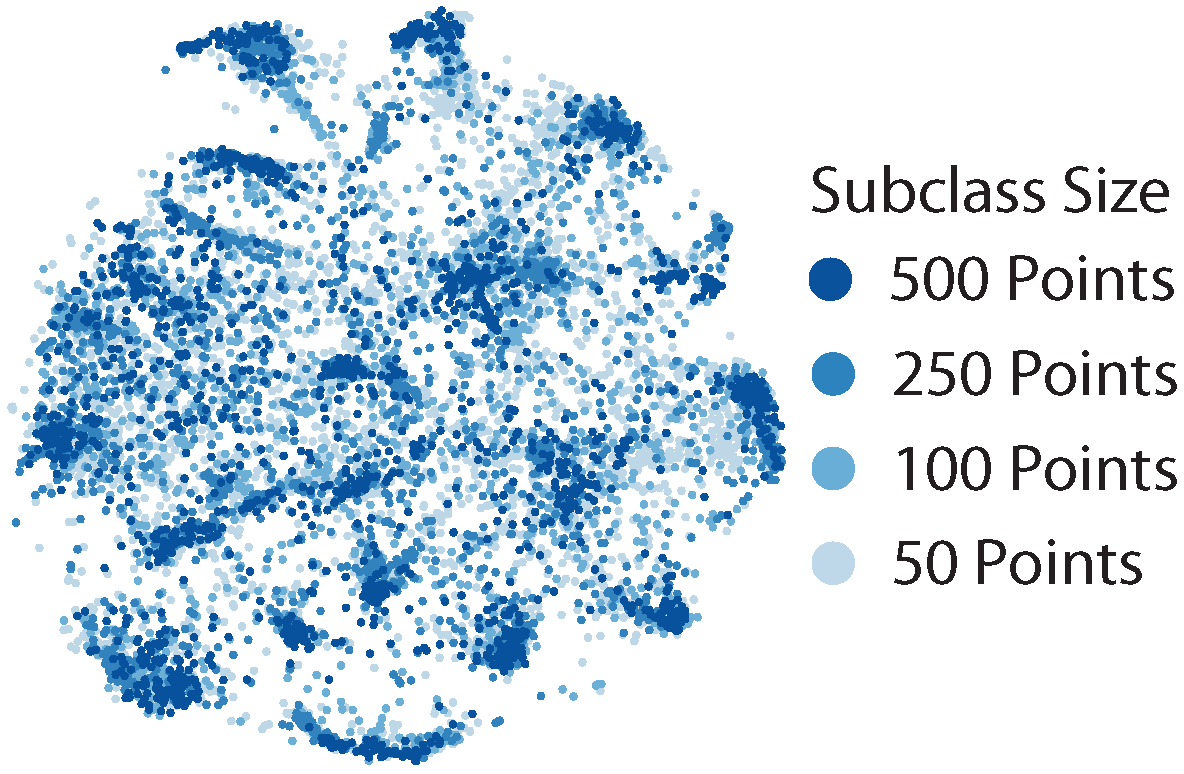
• CIFAR100-Coarse consists of twenty superclasses. We artificially imbalance subclasses to create CIFAR100-Coarse-U. For each superclass, we select one subclass to keep all 500 points, select one subclass to subsample to 250 points, select one subclass to subsample to 100 points, and select the remaining two to subsample to 50 points. We use the original CIFAR100 class index to select which subclasses to subsample: the subclass with the lowest original class index keeps all 500 points, the next subclass keeps 250 points, etc.
• MNIST-Coarse consists of two superclasses: <5 and ≥5.
• Waterbirds [14] is a robustness dataset designed to evaluate the effects of spurious correlations on model performance. The waterbirds dataset is constructed by cropping out birds from photos in the Caltech-UCSD Birds dataset [43], and pasting them on backgrounds from the Places dataset [44]. It consists of two categories: water birds and land birds. The water birds are heavily correlated with water backgrounds and the land birds with land backgrounds, but 5% of the water birds are on land backgrounds, and 5% of the land birds are on water backgrounds. These form the (imbalanced) hidden strata.
• ISIC is a public skin cancer dataset for classifying skin lesions [15] as malignant or benign. 48% of the benign images contain a colored patch, which form the hidden strata.
• CelebA is an image dataset commonly used as a robustness benchmark [14,16]. The task is blonde/not blonde classification. Only 6% of blonde faces are male, which creates a rare stratum in the blonde class.

Appendix E.2. Hyperparameters

For all model quality experiments for $L_{spread}$, we first fixed $\tau =0.5$ and swept $\alpha \in [0.16,0.25,0.33,0.5,0.67]$. We then took the two best-performing values and swept $\tau \in [0.1,0.3,0.5,0.7,0.9]$. For $L_{SC}$ and $L_{SS}$, we swept $\tau \in [0.1,0.3,0.5,0.7,0.9]$. Final hyperparameter values for $(\tau ,\alpha )$ for $L_{spread}$ were $(0.9,0.67)$ for CIFAR10, $(0.5,0.16)$ for CIFAR10-coarse, $(0.5,0.33)$ for CIFAR100, $(0.5,0.25)$ for CIFAR100-Coarse, $(0.5,0.25)$ for CIFAR100-Coarse-U, $(0.5,0.5)$ for MNIST, $(0.5,0.5)$ for MNIST-coarse, $(0.5,0.5)$ for ISIC, and $(0.5,0.5)$ for waterbirds.

For coarse-to-fine transfer learning, we fixed $\tau =0.5$ for all losses and swept $\alpha \in [0.16,0.25,0.33,0.5,0.67]$. Final hyperparameter values for $\alpha$ were $0.25$ for CIFAR10-Coarse, $0.25$ for CIFAR100-Coarse, $0.25$ for CIFAR100-Coarse-U, and $0.5$ for MNIST-Coarse.

Appendix E.3. Applications

We describe additional experimental details for the applications.

Appendix E.3.1. Robustness against Worst-Group Performance

We follow the evaluation of [5]. First, we train a model on the standard class labels. We evaluate different loss functions for this step, including $L_{spread}$, $L_{SC}$, and the cross entropy loss $L_{CE}$. Then we project embeddings of the training set using a UMAP projection [45], and cluster points to discover unlabeled subgroups. Finally, we use the unlabeled subgroups in a Group-DRO algorithm to optimize worst-group robustness [14].

Appendix E.3.2. Robustness against Noise

We use the same training setup as we use to evaluate model quality, and introduce symmetric noise into the labels for the contrastive loss head. We train the cross entropy head with a fraction of the full training set. In Section 5.3, we report results from training with 20% labels to cross entropy. We report additional levels in Appendix F.

We detect noisy labels with a simple geometric heuristic: for each point, we compute the cosine similarity between the embedding of the point and the center of all the other points in the batch that have the same class. We compare this similarity value to the average cosine similarity with points in the batch from every other class, and rank the points by the difference between these two values. Points with incorrect labels have a small difference between these two values (they appear to be small strata, so they are far away from points of the same class). Given the noise level $ϵ$ as an input, we rank the points by this heuristic and mark the $ϵ$ fraction of the batch with the smallest scores as noisy. We then correct their labels by adopting the label of the closest cluster center.

Appendix E.3.3. Minimal Coreset Construction

We use the publicly-available evaluation framework for coresets from [18] (https://github.com/mtoneva/example_forgetting, accessed on 1 October 2021). We use the official repository from [19] (https://github.com/mansheej/data_diet, accessed on 1 October 2021) to recreate their coreset algorithms.

Our coreset algorithm proceeds in two parts. First, we give each point a difficulty rating based on how likely we are to classify it correctly under partial training. Then we subsample the easiest points to construct minimal coresets.

First, we mirror the set up from our thought experiment and train with $L_{spread}$ on random samples of $t\%$ of the CIFAR10 training set, taking three random samples for each of $t\in [10,20,50]$ (and we train the cross entropy head with 1% labeled data). For each run, we record which points are classified correctly by the cross entropy head at the end of training, and bucket points the training set by how often the point was correctly classified. To construct a coreset of size $t\%$, we iteratively remove points from the largest bucket in each class. Our strategy removes easy examples first from the largest coresets, but maintains a set of easy examples in the smallest coresets.

Appendix F.1. Performance of $L_{attract}$

In an early iteration of this project, we experienced success with using $L_{attract}$ on its own to train models, before realizing the benefits of adding in an additional term to prevent class collapse. As an ablation, we report on the performance of using $L_{attract}$ on its own in Table A2. $L_{attract}$ can outperform $L_{SC}$, but $L_{spread}$ outperforms both. We do not report the results here, but $L_{attract}$ also performs significantly worse than $L_{SC}$ on downstream applications, since it more direclty encourages class collapse.

Table A2. Performance of $L_{spread}$ compared to $L_{SC}$ and using $L_{attract}$ on its own. Best in bold.

	End Model Perf.
Dataset	${\mathit{L}}_{\mathbf{SS}}$	${\mathit{L}}_{\mathbf{SC}}$	${\mathit{L}}_{\mathbf{attract}}$	${\mathit{L}}_{\mathbf{spread}}$
CIFAR10	89.7	90.9	91.3	91.5
CIFAR100	68.0	67.5	68.9	69.1

Table A2. Performance of $L_{spread}$ compared to $L_{SC}$ and using $L_{attract}$ on its own. Best in bold.

	End Model Perf.
Dataset	${\mathit{L}}_{\mathbf{SS}}$	${\mathit{L}}_{\mathbf{SC}}$	${\mathit{L}}_{\mathbf{attract}}$	${\mathit{L}}_{\mathbf{spread}}$
CIFAR10	89.7	90.9	91.3	91.5
CIFAR100	68.0	67.5	68.9	69.1

Appendix F.2. Sample Complexity

Figure A1 shows the performance of training ViT models with various amounts of labeled data for $L_{spread}$, $L_{SC}$, and $L_{SS}$. In these experiments, we train the cross entropy head with 1% labeled data to isolate the effect of training data on the contrastive losses themselves.

$L_{spread}$ outperforms $L_{SC}$ and $L_{SS}$ throughout. At 10% labeled data, $L_{spread}$ outperforms $L_{SS}$ by 13.9 points, and outperforms $L_{SC}$ by 0.5 points. By 100% labeled data (for the contrastive head), $L_{spread}$ outperforms $L_{SS}$ by 25.4 points, and outperforms $L_{SC}$ by 10.3 points.

Figure A1. Performance of training ViT with $L_{spread}$ compared to training with $L_{SC}$ and $L_{SS}$ on CIFAR10 at various amounts of labeled data. $L_{spread}$ outperforms the baselines at each point. The cross entropy head here is trained with 1% labeled data to isolate the effect of training data on the contrastive losses.

Appendix F.3. Noisy Labels

In Section 5.3, we reported results from training the contrastive loss head with noisy labels and the cross entropy loss with clean labels from 20% of the training data.

In this section, we first discuss a de-noising algorithm inspired by [23] that we initially developed to correct for noisy labels, but that we did not observe strong empirical results from. We hope that reporting this result inspires future work into improving contrastive learning.

We then report additional results with larger amounts of training data for the cross entropy head.

Appendix F.3.1. Debiasing Noisy Contrastive Loss

First, we consider the triplet loss and show how to debias it in expectation under noise. Then we present an extension to supervised contrastive loss.

Noise-Aware Triplet Loss

Consider the triplet loss:

$$\begin{array}{cc}\hfill L_{triplet}& ={\mathbb{E}}_{\begin{array}{c}x\sim \mathcal{P},x^{+}\sim p^{+}(·|x),\\ x^{-}\sim p^{-}(·|x)\end{array}}-log\frac{exp\left(\sigma (x,x^{+})\right)}{exp\left(\sigma (x,x^{+})\right)+exp\left(\sigma (x,x^{-})\right)}.\hfill \end{array}$$

(A7)

Now suppose that we do not have access to true labels but instead have noisy labels denoted by the weak classifier $\tilde{y}:=\tilde{h}\left(x\right)$. We adopt a simple model of symmetric noise where $\tilde{p}=Pr\left(\mathrm{noisy}\mathrm{label}\mathrm{is}\mathrm{correct}\right)$.

We use $\tilde{y}$ to construct ${\tilde{\mathcal{P}}}^{+}$ and ${\tilde{\mathcal{P}}}^{-}$ as $p\left(x^{+}\right|\tilde{h}\left(x\right)=\tilde{h}\left(x^{+}\right))$ and $p\left(x^{-}\right|\tilde{h}\left(x\right)\ne \tilde{h}\left(x^{-}\right))$. For simplicity, we start by looking at how the triplet loss in (A7) is impacted when noise is not addressed in the binary setting. Define $L_{noisy}^{triplet}$ as $L_{triplet}$ used with ${\tilde{\mathcal{P}}}^{+}$ and ${\tilde{\mathcal{P}}}^{-}$.

Lemma A3.

When class-conditional noise is uncorrected, $L_{triplet}^{noisy}$ is equivalent to

$$\begin{array}{cc}\hfill ({\tilde{p}}^3+{(1-\tilde{p})}^3)L_{triplet}& +\tilde{p}(1-\tilde{p}){\mathbb{E}}_{\begin{array}{c}x\sim \mathcal{P},\\ x_1^{+},x_2^{+}\sim p^{+}(·|x)\end{array}}\left[-log\frac{exp\left(\sigma (x,x_1^{+})\right)}{exp\left(\sigma (x,x_1^{+})\right)+exp\left(\sigma (x,x_2^{+})\right)}\right]\hfill \\ \hfill & +\tilde{p}(1-\tilde{p}){\mathbb{E}}_{\begin{array}{c}x\sim \mathcal{P},\\ x_1^{-},x_2^{-}\sim p^{-}(·|x)\end{array}}\left[-log\frac{exp\left(\sigma (x,x_1^{-})\right)}{exp\left(\sigma (x,x_1^{-})\right)+exp\left(\sigma (x,x_2^{-})\right)}\right]\hfill \\ \hfill & +\tilde{p}(1-\tilde{p}){\mathbb{E}}_{\begin{array}{c}x\sim \mathcal{P},\\ x^{+}\sim p^{+}(·|x)\\ x^{-}\sim p^{-}(·|x)\end{array}}\left[-log\frac{exp\left(\sigma (x,x^{-})\right)}{exp\left(\sigma (x,x^{+})\right)+exp\left(\sigma (x,x^{-})\right)}\right].\hfill \end{array}$$

Proof. 

We split $L_{triplet}^{noisy}$ depending on if the noisy positive and negative pairs are truly positive and negative.

$$\begin{array}{cc}\hfill L_{triplet}^{noisy}& ={\mathbb{E}}_{\begin{array}{c}x\sim \mathcal{P},\\ {\tilde{x}}^{+}\sim {\tilde{p}}^{+}(·|x)\\ {\tilde{x}}^{-}\sim {\tilde{p}}^{-}(·|x)\end{array}}\left[-log\frac{exp\left(\sigma (x,{\tilde{x}}^{+})\right)}{exp\left(\sigma (x,{\tilde{x}}^{+})\right)+exp\left(\sigma (x,{\tilde{x}}^{-})\right)}\right]\hfill \\ \hfill & =p(h\left(x\right)=h\left({\tilde{x}}^{+}\right),h\left(x\right)\ne h\left({\tilde{x}}^{-}\right)){\mathbb{E}}_{\begin{array}{c}x\sim \mathcal{P},\\ x^{+}\sim p^{+}(·|x)\\ x^{-}\sim p^{-}(·|x)\end{array}}\left[-log\frac{exp\left(\sigma (x,x^{+})\right)}{exp\left(\sigma (x,x^{+})\right)+exp\left(\sigma (x,x^{-})\right)}\right]\hfill \\ \hfill & +p(h\left(x\right)=h\left({\tilde{x}}^{+}\right),h\left(x\right)=h\left({\tilde{x}}^{-}\right)){\mathbb{E}}_{\begin{array}{c}x\sim \mathcal{P},\\ x_1^{+},x_2^{+}\sim p^{+}(·|x)\end{array}}\left[-log\frac{exp\left(\sigma (x,x_1^{+})\right)}{exp\left(\sigma (x,x_1^{+})\right)+exp\left(\sigma (x,x_2^{+})\right)}\right]\hfill \\ \hfill & +p(h\left(x\right)\ne h\left({\tilde{x}}^{+}\right),h\left(x\right)\ne h\left({\tilde{x}}^{-}\right)){\mathbb{E}}_{\begin{array}{c}x\sim \mathcal{P},\\ x_1^{-},x_2^{-}\sim p^{-}(·|x)\end{array}}\left[-log\frac{exp\left(\sigma (x,x_1^{-})\right)}{exp\left(\sigma (x,x_1^{-})\right)+exp\left(\sigma (x,x_2^{-})\right)}\right]\hfill \\ \hfill & +p(h\left(x\right)\ne h\left({\tilde{x}}^{+}\right),h\left(x\right)=h\left({\tilde{x}}^{-}\right)){\mathbb{E}}_{\begin{array}{c}x\sim \mathcal{P},\\ x^{+}\sim p^{+}(·|x)\\ x^{-}\sim p^{-}(·|x)\end{array}}[-log\frac{exp\left(\sigma (x,x^{-})\right)}{exp\left(\sigma (x,x^{+})\right)+exp\left(\sigma (x,x^{-})\right)}.]\hfill \end{array}$$

Define $\tilde{p}=p\left(\mathrm{noisy}\mathrm{label}\mathrm{is}\mathrm{correct}\right)$. Note that

$$\begin{array}{c}\hfill p(h\left(x\right)=h\left({\tilde{x}}^{+}\right),h\left(x\right)\ne h\left({\tilde{x}}^{-}\right))={\tilde{p}}^3+{(1-\tilde{p})}^3,\end{array}$$

(i.e., all three points are correct or all reversed, such that their relative pairings are correct). In addition, the other three probabilities above are all equal to $\tilde{p}(1-\tilde{p})$. □

We now show that there exists a weighted loss function that in expectation equals $L_{triplet}$.

Lemma A4.

Define

$$\begin{array}{cc}\hfill & {\tilde{L}}_{triplet}={\mathbb{E}}_{\begin{array}{c}x\sim \mathcal{P},\\ {\tilde{x}}_1^{+},{\tilde{x}}_2^{+}\sim {\tilde{\mathcal{P}}}^{+}(·|x)\\ {\tilde{x}}_1^{-},{\tilde{x}}_2^{-}\sim {\tilde{\mathcal{P}}}^{-}(·|x)\end{array}}[-w^{+}\sigma (x,{\tilde{x}}_1^{+})+w^{-}\sigma (x,{\tilde{x}}_1^{-})\hfill \\ \hfill & +w_{1}log\left(exp\left(\sigma (x,{\tilde{x}}_1^{+})\right)+exp\left(\sigma (x,{\tilde{x}}_1^{-})\right)\right)\hfill \\ \hfill & -w_{2}log\left((exp\left(\sigma (x,{\tilde{x}}_1^{+})\right)+exp\left(\sigma (x,{\tilde{x}}_2^{+})\right))·(exp\left(\sigma (x,{\tilde{x}}_1^{-})\right)+exp\left(\sigma (x,{\tilde{x}}_2^{-})\right))\right)],\hfill \end{array}$$

where

$$\begin{array}{c}\hfill w^{+}=\frac{{\tilde{p}}^2+{(1-\tilde{p})}^2}{{(2\tilde{p}-1)}^2}{w}^{-}=\frac{2\tilde{p}(1-\tilde{p})}{{(2\tilde{p}-1)}^2}{w}_1=\frac{{\tilde{p}}^2+{(1-\tilde{p})}^2}{{(2\tilde{p}-1)}^2}{w}_2=\frac{\tilde{p}(1-\tilde{p})}{{(2\tilde{p}-1)}^2}.\end{array}$$

Then, $\mathbb{E}\left[{\tilde{L}}_{triplet}\right]=L_{triplet}$.

Proof. 

We evaluate $\mathbb{E}\left[-w_1\sigma (x,{\tilde{x}}_1^{+})+w_2\sigma (x,{\tilde{x}}_1^{-})\right]$ and the other terms separately. Using the same probabilities as computed in Lemma A3,

$$\begin{array}{cc}\hfill & \mathbb{E}\left[-w_1\sigma (x,{\tilde{x}}_1^{+})+w_2\sigma (x,{\tilde{x}}_1^{-})\right]=-({\tilde{p}}^2+{(1-\tilde{p})}^2)w_1\mathbb{E}\left[\sigma (x,x_1^{+})\right]\hfill \\ \hfill & -2\tilde{p}(1-\tilde{p})w_1\mathbb{E}\left[\sigma (x,x_1^{-})\right]+({\tilde{p}}^2+{(1-\tilde{p})}^2)w_2\mathbb{E}\left[\sigma (x,x_1^{-})\right]+2\tilde{p}(1-\tilde{p})w_2\mathbb{E}\left[\sigma (x,x_1^{+})\right]\hfill \\ \hfill & =-\sigma (x,x_1^{+}).\hfill \end{array}$$

We evaluate the remaining terms:

$$\begin{array}{ccc}\hfill & \mathbb{E}\left[w_{3}log\left(exp\left(\sigma (x,{\tilde{x}}_1^{+})\right)+exp\left(\sigma (x,{\tilde{x}}_1^{-})\right)\right)\right]=\hfill & \\ \hfill & ({\tilde{p}}^2+{(1-\tilde{p})}^2)w_3\mathbb{E}\left[log\left(exp\left(\sigma (x,x_1^{+})\right)+exp\left(\sigma (x,x_1^{-})\right)\right)\right]\hfill \\ \hfill & +\tilde{p}(1-\tilde{p})w_3\mathbb{E}\left[log\left((exp\left(\sigma (x,{\tilde{x}}_1^{+})\right)+exp\left(\sigma (x,{\tilde{x}}_2^{+})\right))·(exp\left(\sigma (x,{\tilde{x}}_1^{-})\right)+exp\left(\sigma (x,{\tilde{x}}_2^{-})\right))\right)\right].\hfill \end{array}$$

and

$$\begin{array}{cc}\hfill & \mathbb{E}\left[w_{4}log\left(exp\left(\sigma (x,{\tilde{x}}_1^{+})\right)+exp\left(\sigma (x,{\tilde{x}}_2^{+})\right)\right)\right]\hfill \\ \hfill & +\mathbb{E}\left[w_{4}log\left(exp\left(\sigma (x,{\tilde{x}}_1^{-})\right)+exp\left(\sigma (x,{\tilde{x}}_2^{-})\right)\right)\right]=\hfill & \\ \hfill & ({\tilde{p}}^2+{(1-\tilde{p})}^2)w_4\mathbb{E}\left[log\left(exp\left(\sigma (x,x_1^{+})\right)+exp\left(\sigma (x,x_2^{+})\right)\right)\right]\hfill \\ \hfill & +4\tilde{p}(1-\tilde{p})w_4\mathbb{E}\left[log\left(exp\left(\sigma (x,x_1^{+})\right)+exp\left(\sigma (x,x_1^{-})\right)\right)\right]\hfill \\ \hfill & +({(1-\tilde{p})}^2+{\tilde{p}}^2)w_4\mathbb{E}\left[log\left(exp\left(\sigma (x,x_1^{-})\right)+exp\left(\sigma (x,x_2^{-})\right)\right)\right].\hfill \end{array}$$

Examining the coefficients, we see that

$$\begin{array}{cc}\hfill & ({\tilde{p}}^2+{(1-\tilde{p})}^2)w_3-4\tilde{p}(1-\tilde{p})w_4=\frac{{({\tilde{p}}^2+{(1-\tilde{p})}^2)}^2}{{(2\tilde{p}-1)}^2}-\frac{4{\tilde{p}}^2{(1-\tilde{p})}^2}{{(2\tilde{p}-1)}^2}=1\hfill \\ \hfill & \tilde{p}(1-\tilde{p})w_3-({\tilde{p}}^2+{(1-\tilde{p})}^2)w_4=\frac{\tilde{p}(1-\tilde{p})({\tilde{p}}^2+{(1-\tilde{p})}^2)}{{(2\tilde{p}-1)}^2}-\frac{({\tilde{p}}^2+{(1-\tilde{p})}^2)\tilde{p}(1-\tilde{p})}{{(2\tilde{p}-1)}^2}=0,\hfill \end{array}$$

which shows that only the term $\mathbb{E}\left[log\left(exp\left(\sigma (x,x_1^{+})\right)+exp\left(\sigma (x,x_1^{-})\right)\right)\right]$ persists. This completes our proof. □

We now show the general case for debiasing $L_{attract}$, which uses more negative samples.

Proposition A1.

Define $m=n+1$ (as the “batch size” in the denominator), and

$$\begin{array}{cc}\hfill {\tilde{L}}_{attract}& ={\mathbb{E}}_{\begin{array}{c}x\sim \mathcal{P}\\ {\left\{{\tilde{x}}_i^{+}\right\}}_{i=1}^m\\ {\left\{{\tilde{x}}_j^{-}\right\}}_{j=1}^m\end{array}}[-w^{+}\sigma (x,{\tilde{x}}_1^{+})+w^{-}\sigma (x,{\tilde{x}}_1^{-})\hfill \end{array}$$

(A8)

$$\begin{array}{cc}\hfill & +\sum _{k=0}^m{w}_{k}log\left(\sum _{i=1}^{k}exp\left(\sigma (x,{\tilde{x}}_i^{+})\right)+\sum _{j=1}^{m-k}exp\left(\sigma (x,{\tilde{x}}_j^{-})\right)\right)].\hfill \end{array}$$

(A9)

$w^{+}$ and $w^{-}$ are defined in the same was as before. $\overrightarrow{w}=\{w_0,\cdots w_m\}\in {\mathbb{R}}^{m+1}$ is the solution to the system $\mathbf{P}w={\mathbf{e}}_2$ where ${\mathbf{e}}_2$ is the standard basis vector in ${\mathbb{R}}^{m+1}$ where the 2nd index is 1 and all others are 0. The $i,j$th element of $\mathbf{P}$ is ${\mathbf{P}}_{ij}=\tilde{p}{\mathbf{Q}}_{i,j}+(1-\tilde{p}){\mathbf{Q}}_{m-i,j}$ where

$$\begin{array}{c}\hfill {\mathbf{Q}}_{i,j}=\left\{\begin{array}{cc}\sum _{k=0}^{min\{j,m-i\}}\left(\genfrac{}{}{0pt}{}{j}{k}\right)\left(\genfrac{}{}{0pt}{}{m-j}{i-j+k}\right){(1-\tilde{p})}^{i-j+2k}{\tilde{p}}^{m+j-i-2k}\hfill & j\le i\hfill \\ \sum _{k=0}^{min\{i,m-j\}}\left(\genfrac{}{}{0pt}{}{m-j}{k}\right)\left(\genfrac{}{}{0pt}{}{j}{j-i+k}\right){(1-\tilde{p})}^{j-i+2k}{\tilde{p}}^{m-j+i-2k}\hfill & j>i\hfill \end{array}\right.\end{array}$$

Then, $\mathbb{E}\left[{\tilde{L}}_{attract}\right]=L_{attract}$.

We do not present the proof for Proposition A1, but the steps are very similar to the proof for the triplet loss case. We also note that a different form of $\mathbb{E}\left[{\tilde{L}}_{attract}\right]$ must be computed for the multi-class case, which we do not present here (but can be derived through computation).

Observation A2.

Note that the values of ${\mathbf{Q}}_{\mathbf{i},\mathbf{j}}$ have high variance in the noise rate as m increases. Additionally, note that the number of terms in the summation of ${\mathbf{Q}}_{\mathbf{i},\mathbf{j}}$ increase combinatorially with m. We found this de-noising algorithm very unstable as a result.

Appendix F.3.2. Additional Noisy Label Results

Now we report the performance of denoising algorithms with additional amounts of labeled data for the cross entropy loss head. We also report the performance of using ${\tilde{L}}_{attract}$ to debias noisy labels.

Figure A2 shows the results. Our geometric correction together with $L_{spread}$ works the most consistently. Using the geometric correction with $L_{SC}$ can be unreliable, since $L_{SC}$ can learn memorize noisy labels early on in training. The expectation-based debiasing algorithm ${\tilde{L}}_{attract}$ occasionally shows promise but is unreliable, and is very sensitive to having the correct noise rate as an input.

Figure A2. Performance of models under various amounts of label noise for the contrastive loss head, and various amounts of clean training data for the cross entropy loss.

References

- Khosla, P.; Teterwak, P.; Wang, C.; Sarna, A.; Tian, Y.; Isola, P.; Mschinot, A.; Liu, C.; Krishnan, D. Supervised Contrastive Learning. Adv. Neural Inf. Process. Syst. 2020, 33, 18661–18673. [Google Scholar]
- Graf, F.; Hofer, C.; Niethammer, M.; Kwitt, R. Dissecting Supervised Constrastive Learning. Proc. Int. Conf. Mach. Learn. PMLR. 2021, 139, 3821–3830. [Google Scholar]
- Zhang, C.; Bengio, S.; Hardt, M.; Recht, B.; Vinyals, O. Understanding deep learning requires rethinking generalization. Commun. ACM 2016, 64, 107–115. [Google Scholar] [CrossRef]
- Hoffmann, A.; Kwok, R.; Compton, P. Using subclasses to improve classification learning. In European Conference on Machine Learning; Springer: Berlin/Heidelberg, Germany, 2001; pp. 203–213. [Google Scholar]
- Sohoni, N.; Dunnmon, J.; Angus, G.; Gu, A.; Ré, C. No Subclass Left Behind: Fine-Grained Robustness in Coarse-Grained Classification Problems. Adv. Neural Inf. Process. Syst. 2020, 33, 19339–19352. [Google Scholar]
- Oakden-Rayner, L.; Dunnmon, J.; Carneiro, G.; Ré, C. Hidden stratification causes clinically meaningful failures in machine learning for medical imaging. In Proceedings of the Proceedings of the ACM conference on Health, Inference, and Learning, Toronto, ON, Canada, 2–4 April 2020; pp. 151–159. [Google Scholar]
- Linsker, R. Self-organization in a perceptual network. Computer 1988, 21, 105–117. [Google Scholar] [CrossRef]
- Wang, T.; Isola, P. Understanding contrastive representation learning through alignment and uniformity on the hypersphere. Proc. Int. Conf. Mach. Learn. PMLR 2020, 119, 9929–9939. [Google Scholar]
- Robinson, J.; Chuang, C.Y.; Sra, S.; Jegelka, S. Contrastive learning with hard negative samples. arXiv 2020, arXiv:2010.04592. [Google Scholar]
- Ben-David, S.; Blitzer, J.; Crammer, K.; Kulesza, A.; Pereira, F.; Vaughan, J.W. A theory of learning from different domains. Mach. Learn. 2010, 79, 151–175. [Google Scholar] [CrossRef] [Green Version]
- Ben-David, S.; Blitzer, J.; Crammer, K.; Pereira, F. Analysis of representations for domain adaptation. Adv. Neural Inf. Process. Syst. 2007, 19, 137. [Google Scholar]
- Ben-David, S.; Urner, R. On the Hardness of Domain Adaptation and the Utility of Unlabeled Target Samples. In Proceedings of the 23rd International Conference, Lyon, France, 29–31 October 2012; Bshouty, N.H., Stoltz, G., Vayatis, N., Zeugmann, T., Eds.; Springer: Berlin/Heidelberg, Germany, 2012; pp. 139–153. [Google Scholar]
- Mansour, Y.; Mohri, M.; Rostamizadeh, A. Domain adaptation: Learning bounds and algorithms. arXiv 2009, arXiv:0902.3430. [Google Scholar]
- Sagawa, S.; Koh, P.W.; Hashimoto, T.B.; Liang, P. Distributionally Robust Neural Networks for Group Shifts: On the Importance of Regularization for Worst-Case Generalization. arXiv 2019, arXiv:1911.08731. [Google Scholar]
- Codella, N.; Rotemberg, V.; Tschandl, P.; Celebi, M.E.; Dusza, S.; Gutman, D.; Helba, B.; Kalloo, A.; Liopyris, K.; Marchetti, M.; et al. Skin lesion analysis toward melanoma detection 2018: A challenge hosted by the international skin imaging collaboration (isic). arXiv 2019, arXiv:1902.03368. [Google Scholar]
- Liu, Z.; Luo, P.; Wang, X.; Tang, X. Deep Learning Face Attributes in the Wild. In Proceedings of the Proceedings of International Conference on Computer Vision (ICCV), Santiago, Chile, 7 December 2015. [Google Scholar]
- Dosovitskiy, A.; Beyer, L.; Kolesnikov, A.; Weissenborn, D.; Zhai, X.; Unterthiner, T.; Dehghani, M.; Minderer, M.; Heigold, G.; Gelly, S.; et al. An Image is Worth 16x16 Words: Transformers for Image Recognition at Scale. arXiv 2020, arXiv:2010.11929. [Google Scholar]
- Toneva, M.; Sordoni, A.; des Combes, R.T.; Trischler, A.; Bengio, Y.; Gordon, G.J. An Empirical Study of Example Forgetting during Deep Neural Network Learning. arXiv 2018, arXiv:1812.05159. [Google Scholar]
- Paul, M.; Ganguli, S.; Dziugaite, G.K. Deep Learning on a Data Diet: Finding Important Examples Early in Training. arXiv 2021, arXiv:2107.07075. [Google Scholar]
- Chen, T.; Kornblith, S.; Norouzi, M.; Hinton, G. A simple framework for contrastive learning of visual representations. Proc. Int. Conf. Mach. Learn. PMLR 2020, 119, 1597–1607. [Google Scholar]
- Arora, S.; Khandeparkar, H.; Khodak, M.; Plevrakis, O.; Saunshi, N. A theoretical analysis of contrastive unsupervised representation learning. arXiv 2019, arXiv:1902.09229. [Google Scholar]
- Zimmermann, R.S.; Sharma, Y.; Schneider, S.; Bethge, M.; Brendel, W. Contrastive Learning Inverts the Data Generating Process. arXiv 2021, arXiv:2012.08850. [Google Scholar]
- Chuang, C.Y.; Robinson, J.; Torralba, A.; Jegelka, S. Debiased Contrastive Learning. Adv. Neural Inf. Process. Syst. 2020, 33, 8765–8775. [Google Scholar]
- Oord, A.v.d.; Li, Y.; Vinyals, O. Representation learning with contrastive predictive coding. arXiv 2018, arXiv:1807.03748. [Google Scholar]
- Tian, Y.; Sun, C.; Poole, B.; Krishnan, D.; Schmid, C.; Isola, P. What makes for good views for contrastive learning? arXiv 2020, arXiv:2005.10243. [Google Scholar]
- Tsai, Y.H.H.; Wu, Y.; Salakhutdinov, R.; Morency, L.P. Self-supervised Learning from a Multi-view Perspective. arXiv 2020, arXiv:2006.05576. [Google Scholar]
- Tschannen, M.; Djolonga, J.; Rubenstein, P.K.; Gelly, S.; Lucic, M. On Mutual Information Maximization for Representation Learning. arXiv 2019, arXiv:1907.13625. [Google Scholar]
- He, K.; Fan, H.; Wu, Y.; Xie, S.; Girshick, R. Momentum Contrast for Unsupervised Visual Representation Learning. arXiv 2019, arXiv:1911.05722. [Google Scholar]
- Chen, X.; Fan, H.; Girshick, R.; He, K. Improved Baselines with Momentum Contrastive Learning. arXiv 2020, arXiv:2003.04297. [Google Scholar]
- Goyal, P.; Caron, M.; Lefaudeux, B.; Xu, M.; Wang, P.; Pai, V.; Singh, M.; Liptchinsky, V.; Misra, I.; Joulin, A.; et al. Self-supervised Pretraining of Visual Features in the Wild. arXiv 2021, arXiv:2103.01988. [Google Scholar]
- Caron, M.; Misra, I.; Mairal, J.; Goyal, P.; Bojanowski, P.; Joulin, A. Unsupervised Learning of Visual Features by Contrasting Cluster Assignments. Adv. Neural Inf. Process. Syst. 2020, 33, 9912–9924. [Google Scholar]
- Islam, A.; Chen, C.F.; Panda, R.; Karlinsky, L.; Radke, R.; Feris, R. A Broad Study on the Transferability of Visual Representations with Contrastive Learning. arXiv 2021, arXiv:2103.13517. [Google Scholar]
- Bukchin, G.; Schwartz, E.; Saenko, K.; Shahar, O.; Feris, R.; Giryes, R.; Karlinsky, L. Fine-grained Angular Contrastive Learning with Coarse Labels. In Proceedings of the 2021 IEEE/CVF Conference on Computer Vision and Pattern Recognition (CVPR), Virtual, 19 June 2021; 2021. [Google Scholar] [CrossRef]
- d’Eon, G.; d’Eon, J.; Wright, J.R.; Leyton-Brown, K. The Spotlight: A General Method for Discovering Systematic Errors in Deep Learning Models. arXiv 2021, arXiv:2107.00758. [Google Scholar]
- Duchi, J.; Hashimoto, T.; Namkoong, H. Distributionally robust losses for latent covariate mixtures. arXiv 2020, arXiv:2007.13982. [Google Scholar]
- Goel, K.; Gu, A.; Li, Y.; Re, C. Model Patching: Closing the Subgroup Performance Gap with Data Augmentation. arXiv 2020, arXiv:2008.06775. [Google Scholar]
- Liu, S.; Niles-Weed, J.; Razavian, N.; Fernandez-Granda, C. Early-Learning Regularization Prevents Memorization of Noisy Labels. Adv. Neural Inf. Process. Syst. 2020, 33, 20331–20342. [Google Scholar]
- Li, J.; Xiong, C.; Hoi, S.C. Semi-supervised Learning with Contrastive Graph Regularization. In Proceedings of the IEEE/CVF International Conference on Computer Vision (ICCV), Virtual, 11 October 2021. [Google Scholar]
- Ciortan, M.; Dupuis, R.; Peel, T. A Framework using Contrastive Learning for Classification with Noisy Labels. arXiv 2021, arXiv:2104.09563. [Google Scholar] [CrossRef]
- Li, J.; Socher, R.; Hoi, S.C. DivideMix: Learning with Noisy Labels as Semi-supervised Learning. arXiv 2020, arXiv:2002.07394. [Google Scholar]
- Ju, J.; Jung, H.; Oh, Y.; Kim, J. Extending Contrastive Learning to Unsupervised Coreset Selection. arXiv 2021, arXiv:2103.03574. [Google Scholar] [CrossRef]
- Sener, O.; Savarese, S. Active Learning for Convolutional Neural Networks: A Core-Set Approach. arXiv 2017, arXiv:1708.00489. [Google Scholar]
- Welinder, P.; Branson, S.; Mita, T.; Wah, C.; Schroff, F.; Belongie, S.; Perona, P. Caltech-UCSD Birds 200. In Technical Report CNS-TR-2010-001; California Institute of Technology: Pasadena, CA, USA, 2010. [Google Scholar]
- Zhou, B.; Lapedriza, A.; Xiao, J.; Torralba, A.; Oliva, A. Learning Deep Features for Scene Recognition using Places Database. Adv. Neural Inf. Process. Syst. 2014, 27, 487–495. [Google Scholar]
- McInnes, L.; Healy, J.; Saul, N.; Großberger, L. UMAP: Uniform Manifold Approximation and Projection. J. Open Source Softw. 2018, 3. [Google Scholar] [CrossRef]