Drift and Diffusion in Panel Data: Extracting Geopolitical and Temporal Effects in a Study of Passenger Rail Traffic ^†

Abstract

Two-stage least squares (2SLS) regression undergirds much of contemporary geospatial econometrics. Walk-forward validation in time-series forecasting constitutes a special instance of iterative local regression. Two-stage least squares and iterative regression supply distinct approaches to isolating the drift and diffusion terms in data containing deterministic and stochastic components. To demonstrate the benefits of these methods outside their native contexts, this paper applies 2SLS correction of residuals and iterative local regression to panel data on passenger railway traffic in Europe. Goodness of fit improved from r² ≈ 0.685 to r² ≈ 0.723 through 2SLS and to r² ≈ 0.825 through iterative local regression. Two-stage least squares provides strong evidence of geopolitical and temporal influences. Iterative local regression produces implicit vectors of coefficients and p-values that reinforce some causal inferences of the unconditional model for rail passenger traffic while simultaneously undermining others.

1. Introduction

This paper performs two distinct tasks. Åt a purely mechanical level, this paper extends previous work on railway traffic in Europe [1]. This paper uses two regression methods to improve the accuracy of the previous work’s predictions of European passenger rail traffic (Figure 1). This extension improves the goodness of fit from r² ≈ 0.685 to values ranging from r² ≈ 0.723 to r² ≈ 0.825.

At a second, more theoretical level, this paper validiates a conjecture on the generalizability of methods more commonly found in geospatial econometrics and time-series forecasting [2]. Two-stage least squares (2SLS) estimates of residuals often reveal spatial dependencies within geospatially marked datasets. Many time-series forecasts engage in iterative local regression as they walk forward through rolling forecasting windows. Both methods, in principle, should apply to panel data. This paper applies both methods, dramatically improving predictive accuracy while offering critical commentary on the causal inferences drawn by the underlying analysis.

Part 2 summarizes the underlying work on European passenger rail traffic [1]. It also presents 2SLS and iterative local regression as methods inspired by geospatial econometrics. Part 3 presents results from the 2SLS evaluation of residuals from an unconditional regression of the entire panel dataset. Part 4 presents the results from iterative local regression based on k-means clustering. Part 5 recommends that these methods be applied more broadly in analyses of economic panel data.

2. Previous Work, Materials, and Methods

2.1. Economic Determinants of European Railway Traffic

An application of traditional and machine-enhanced methods concluded that the size of the rail network, the gross domestic product per capita, and the fertility rate have a positive and statistically significant impact on per capita passenger traffic in the European Union [1]. Unemployment has a negative impact.

Table 1. Parameter estimates for macroeconomic and industry-specific factors affecting passengers per capita in 25 European Union countries.

Predictive Variable	OLS	Soft Voting
gdp_pc	0.507549 *** 1	0.482761 ***
gdp_growth	−0.056322	−0.040858
inflation	−0.031413	−0.013827
unemployment	−0.206676 ***	−0.196214 ***
fertility	0.112462 *	0.108103 *
network_log	0.612954 ***	0.595888 ***
cars_pc	−0.021308	−0.003860
deaths_pc	−0.037088	−0.011879

¹ Levels of statistical significance—***: p < 0.001; *: p < 0.05.

reports results based on ordinary least squares (OLS) and a soft-voting aggregator that blends a suite of regularized linear regression methods (such as Ridge, Lasso, and their Bayesian equivalents) [3]. As a general rule, those methods’ ℓ₂ and ℓ₁ penalties push parameter estimates toward zero.

This model exhibited visible fixed entity effects (Figure 1). Even the more reliable soft-voting model overestimated the rail passenger traffic in Romania and Ireland and underestimated the traffic in Hungary, Austria, and France. Though hardly extreme, those estimation errors sufficed to classify these five countries collectively as outliers within an otherwise accurate model.

2.2. Drift and Diffusion in Geospatial Econometrics

This project’s companion paper, published elsewhere in these proceedings, examines the median house prices in 20,640 California districts [2]. That paper pursues three strategies to extract, evaluate, and quantify the geospatial component of housing prices:

• Data engineering of predictive variables as a prelude to predictive methods;
• Two-stage least-squares (2SLS) regression of residuals;
• Iterative local regression of instances defined by unsupervised k-nearest neighbors.

The drift and diffusion approach in [4] forgoes the determination of geospatial effects through data engineering, such as the calculation of the distance to the central business district or the location of a tract at a harbor or along the riverfront. Instead, the basic formulation of an unconditional OLS model is decomposed into distinct drift and diffusion components:

y = Xβ + u

(1)

Xβ is the design matrix times all of the parameter estimates. It is equivalent to ŷ, the vector of the fitted values. Xβ also defines the drift term. If Xβ, as a deliberately underfit effort to find ŷ, contains only hedonic variables, then the error term, u, contains geospatial information presumably not addressed in the design matrix.

u is equivalent to the residuals, defined as u = y − ŷ. Geospatial analysis often subjects u to a second-stage regression of its own, u = û − v. This 2SLS regression regards the original error term as the locus of diffusion for all geospatial effects. For the spatial component of any data, û is a function of distance from some reference point. Although geospatial analysis typically applies Haversine distance, other applications may adopt another distance metric. For the temporal component of panel data, û can be evaluated as a function of time.

Finally, the equation y = Xβ + û + v enables the reconstruction of the original model. At least where the second-stage process succeeds in estimating the original set of residuals, substituting the 2SLS equation, u = û − v, for the drift model’s error term improves the overall predictive accuracy. This gain results from the successful capture of stochastic diffusion not captured by deterministic modeling of the drift term.

Relative to 2SLS, iterative local regression inverts the treatment of the drift and diffusion terms. Iterative local regression of geospatial data assumes that the relationship between hedonic and socioeconomic predictors, on one hand, and a target variable such as median house value is more likely to cohere within a geographically circumscribed subset. On the assumption that the geographically closest districts would provide more accurate information, Ref. [2] used unsupervised k-nearest neighbors to supply the initial filtering before producing a series of locally focused regression exercises.

Two-stage least squares and iterative local regression represent conceptually distinct but mutually compatible approaches toward understanding temporal, geospatial, and socioeconomic distances within panel data. The balance of this paper applies 2SLS and iterative local regression to panel data describing passenger rail traffic in Europe.

3. Results, Part 1: Two-Stage Least Squares

Explicit consideration of spatial and temporal effects beyond hedonic or macroeconomic variables dramatically improves predictive accuracy. Since the dataset involves 19 years of annual observations from 25 European Union countries, the political boundaries of the EU provide a convenient starting point. Subdividing the dataset into those countries and years yields a unique categorical label and a year for each of n = 475 observations.

A multistage regression routine based on those divisions begins with straightforward geopolitical and temporal partitions of the data. The balance of this section presents, in turn, the results of a geopolitical 2SLS correction of drift-term residuals and the results of a correction based on the passage of time.

3.1. Geopolitical Distance: A Stylized Vector of “Carolingian Distances”

Some datasets may emphasize geopolitical distance instead of geospatial distance. In some applications involving multiple rounds of regression, the second stage proceeds with a vector of additional predictors numbering more than one [5]. The formal definition of instrumental variable regression explicitly stipulates that the cardinality of a “matrix Z of valid instrumental variables” must equal or exceed the cardinality of endogenous predictors within the original design matrix [6] (p. 557).

Although 2SLS regression is not circumscribed by this constraint on instrumental variables, 2SLS does need to designate at least one variable beyond the predictors already in the design matrix (

Table 2. “Carolingian distances” from Aachen to each of 25 European Union capitals, in kilometers and as z-scores.

Country	“Carolingian Distance” (Kilometers from Aachen) 2	Carolingian Distance Expressed as a Z-Score
Austria	795.36	−0.433695
Belgium	121.51	−1.743004
Bulgaria	1585.75	1.102055
Croatia	915.40	−0.200454
Czechia	595.26	−0.822495
Denmark	694.67	−0.629338
Estonia	1520.40	0.975078
Finland	1572.19	1.075708
France	342.21	−1.314178
Germany	541.48	−0.926991
Greece	1988.79	1.885173
Hungary	1009.08	−0.018431
Ireland	889.91	−0.249981
Italy	1102.83	0.163728
Latvia	1360.59	0.664563
Lithuania	1358.86	0.661201
Luxembourg	129.63	−1.727227
Netherlands	195.79	−1.598676
Poland	1043.88	0.049187
Portugal	1794.42	1.507507
Romania	1651.30	1.229420
Slovakia	847.77	−0.331861
Slovenia	813.07	−0.399284
Spain	1377.94	0.698274
Sweden	1216.05	0.383718

² Source: https://distancecalculator.net (last visited 12 May 2025).

). This study relies on distance from Aachen, the historical seat of the Carolingian Empire. Though it may seem implausible, a single geospatial vector of the distances by air from Aachen to 25 European capitals predicts residuals from the drift-term regression and improves the ultimate goodness of fit. The choice of a central point within a transportation network evokes basing-point pricing, a common but controversial practice in steel, automobile assembly, and other freight-dependent industries [7,8,9].

Table 2 reports this stylized vector of the Carolingian distances for 25 EU countries, in kilometers and in standardized z-scores. The standardized distances in the final column resemble coefficients on dummy variables tracking fixed entity effects. They enable a regression against the country-by-country average value of the target variable.

The results of that second-stage regression are u = 0.001606 − 0.214943x + v, where u represents the residuals in the original unconditional panel regression (or the drift term), x expresses the standardized distance from each country’s capital to the stylized center of Europe in Aachen, and v represents the error term (

Table 3. Correlations between the vector of Carolingian distances (Table 2) and the predictive and target variables in the model of passenger rail traffic.

Predictive Variable	Correlation with Carolingian Distance
gdp_pc	−0.558713 ** 3
gdp_growth	0.077160
inflation	0.346282 +
unemployment	0.534734 **
fertility	−0.385699 +
network_log	0.006705
cars_pc	−0.367631 +
deaths_pc	0.402817 *
passengers	−0.612838 **

³ Levels of statistical significance—**: p < 0.01; *: p < 0.05; +: p < 0.10. No variable attained statistical significance at the conventional threshold of p < 0.001.

). The coefficient −0.214943 is statistically significant according to conventional criteria (p = 0.035185) and implies that each increase of 525.273 km in Carolingian distance reduces passenger rail traffic by 78.374.

Carolingian distances from Aachen to various European capitals have predictive power because this vector correlates with multiple predictors and the target variable in this model of passenger rail traffic (Table 3). The variables in Table 3 refer to country-specific means, which collectively define the centroids for all 25 EU member-states in this study. Curiously, the variable with the lowest correlation to distance from Aachen is the most predictive variable, network_log. But strong correlations elsewhere in the vector of independent variables produce the most important and predictive correlation with Carolingian distance: r = −0.612838 relative to mean passenger traffic by national cohort.

3.2. Correcting Residuals over the Course of Time

A 2SLS correction for time is even simpler. Temporal distance is the difference between the year of an observation and 2000, the earliest year in the dataset. The second-stage regression based on the years 2000 to 2018 yielded the formula u = 0.179776 − 0.019423t + v, where t represents years beyond 2000. The coefficient for t is statistically significant (p = 0.010959).

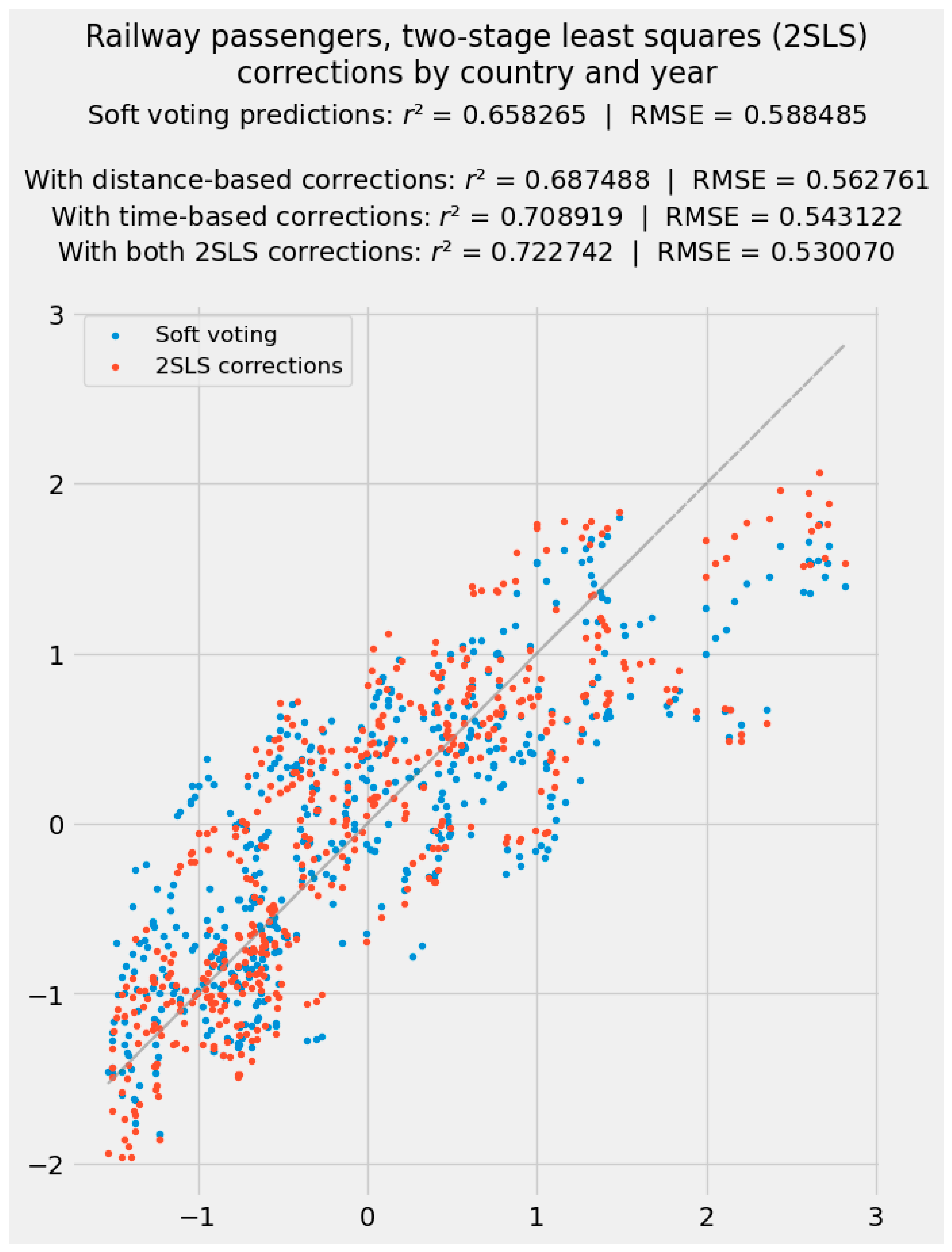
The combined 2SLS correction, including both geospatial and temporal effects, is displayed in Figure 2. The spatial adjustment, though crudely based on distance from a historical capital, improved r² from 0.658265 to 0.687488. In a period of increasing passenger rail travel, temporal corrections on their own improved r² to 0.708919. Combined, the spatial and temporal adjustments raised r² to 0.722742. The corresponding combined reduction in root mean squared error (RMSE) from 0.588485 to 0.430070 represented 9.93 percent of the total RMSE of the original soft-voting model.

This achievement vindicates the conjecture that a 2SLS correction of residuals after unconditional multivariable regression can improve predictive accuracy for panel data [2]. Figure 2 therefore shows how 2SLS, a pivotal method in geospatial analyses [4,10], can be generalized to other domains.

4. Results, Part 2: Clustering and Iterative Local Regression

Part 4 now presents an alternative approach based on unsupervised machine learning. k-means clustering of the entire dataset preprocesses this study of European railway passenger traffic into seven mathematically cogent cohorts. Applying iterative local regression to those clusters yields even greater predictive improvements.

4.1. Fixed Effects as a Form of Clustering

The very idea of clustering is a reminder that the social sciences almost always operate on samples rather than populations. The 475 instances describing European railway passenger traffic by nation and year should not be regarded as an exhaustive and permanent population encompassing all possible observations. Rather, the dataset represents a mere sample, delimited in geopolitical space, as well as time.

The presence of fixed entity or time effects implies that a dataset may not be independent and identically distributed. Moreover, these fixed effects may not be the most mathematically efficient way to partition the data. We may surmise—but cannot know with assurance in the absence of further quantitative evaluation—that Austria in 2000 is more closely related to Austria in 2018 and that both of those observations are more remote from Sweden in 2009. This supposition arises from the assumption that each national cohort represents its own cluster. That definition is convenient and congruent with geopolitical reality. But nothing guarantees its mathematical cogency, let alone optimality.

4.2. K-Means Clustering

Fixed effects are hardly the only way to partition data. Unsupervised machine learning can unveil the internal structure of a dataset. This study relies on k-means clustering [11]. Setting k = 7 followed a brief application of the elbow and silhouette tests [12]. Values of k less than or greater than 7 produced less accurate predictions. Although this might be no more than mere conjecture in the absence of more elaborate theoretical and empirical work, suboptimal predictions may indicate improper clustering.

k-means clustering (k = 7) for this dataset on European railway passenger traffic appears in Figure 3. Multidimensional scaling (MDS), a method of dimensionality reduction through nonlinear manifold learning [13], permits the visually appealing projection of the seven clusters in three dimensions. Clustering proceeded without consideration of the target variable (railway passengers per capita) to prevent this preprocessing method from biasing predictions.

Each of the clusters in Figure 3, numbered 0 through 6, contains a stable subset of observations. Their membership is reported in the Appendix A. Clusters 0, 2, and 5 are dominated by observations throughout eastern and central Europe. The countries in those clusters that were not members of the former Warsaw Pact or parts of former Yugoslavia are the Mediterranean countries of Greece, Spain, and Portugal. Clusters 1, 3, and 4 contain more observations from wealthier countries such as Belgium, France, and Finland. Cluster 6 consists of all observations for Luxembourg, the country that uniquely combines Europe’s highest per capita income with one of the Union’s lowest levels of rail passenger traffic.

Those seven clusters are now amenable to the correction of residuals through iterative local regression (Figure 3). The clusters can be identified by their centroids or a mean value for each independent variable in the design matrix (

Table 4. Centroids for each of seven clusters generated through k-means clustering.

Variables	Cluster 0	Cluster 1	Cluster 2	Cluster 3	Cluster 4	Cluster 5	Cluster 6
gdp_pc	−0.624985	0.275276	−0.414271	0.911555	−0.445655	−1.015505	3.201688
gdp_growth	0.170321	−0.319924	−1.465259	−0.222085	0.239041	1.067098	0.135049
inflation	0.399676	−0.263255	−0.310005	−0.295721	−0.231274	0.850973	−0.174410
unemployment	−0.436845	−0.396739	1.805759	−0.399750	−0.191861	0.744581	−1.012578
fertility	−0.769180	−0.540283	−0.594548	1.363578	0.273314	−0.967505	0.242712
network_log	0.010233	1.013735	−0.267620	0.127315	−0.547535	−0.217838	−2.713473
cars_pc	−0.266320	0.988292	−0.066136	0.318287	−0.067569	−1.284779	1.948569
deaths_pc	1.073907	−0.380362	−0.255050	−0.803224	−0.281161	1.510772	−0.015089

). Heavily eastern European cluster 5, for instance, is distinguished by its unusually low GDP per capita. By contrast, cluster 6 exhibits Luxembourg’s unusual combination of very high GDP per capita and unusually small network size.

4.3. Analytical Results from Iterative Local Regression

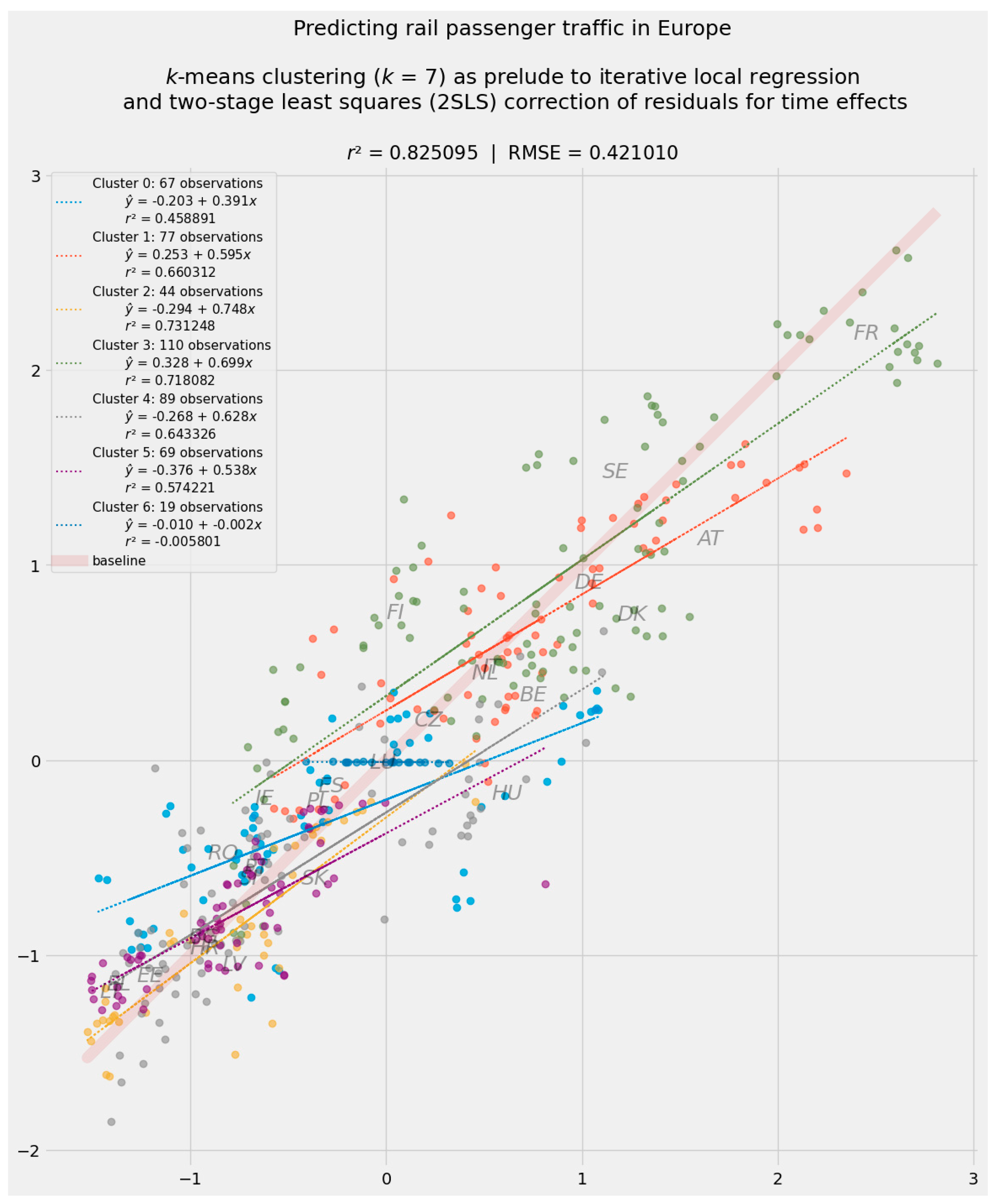
Cluster centroids are not the only indicator of group-specific effects. Iterative local regression of each cluster generates its own set of parameter estimates. A least-angle implementation of Lasso regression [14], optimized according to the Akaike information criterion (Lars or LassoLarsAIC), yielded the best results.

Table 5. Local regression results for each of k = 7 clusters.

Variables	Cluster 0	Cluster 1	Cluster 2	Cluster 3	Cluster 4	Cluster 5	Cluster 6
ℓ1 alpha	0.022699	0.017015	0.006488	0.000000	0.002039	0.004957	0.051609
r2	0.386987	0.639893	0.884457	0.723767	0.694480	0.563336	0.000000
intercept	−0.667326	0.508055	−0.728775	0.546850	0.282417	−0.744207	−0.013269
gdp_pc	0.000000	0.888764	0.000000	0.663217	1.349062	0.000000	0.000000
gdp_growth	0.000000	−0.074480	0.000000	−0.163557	−0.352117	0.000000	0.000000
inflation	0.000000	0.000000	0.000000	−0.249260	0.075187	0.029277	0.000000
unemployment	−0.676279	−0.190030	−0.103394	−0.313400	−0.084758	0.082659	0.000000
fertility	−0.346999	0.000000	−0.089854	−0.259930	0.000000	0.000000	0.000000
network_log	0.401915	0.000000	0.409860	1.126678	0.496841	0.298184	0.000000
cars_pc	0.000000	−0.127164	−0.233341	−0.247714	−0.184285	0.000000	0.000000
deaths_pc	−0.089092	0.000000	−0.284552	0.254671	−0.202252	−0.049151	0.000000

reports Lars alpha (the ℓ₁ penalty), goodness of fit as measured by r², the intercept, and the parameter estimates for each cluster-based regression exercise.

Notably, goodness of fit for local regression did not necessarily exceed r² = 0.658285 in the unconditional soft-voting regression of the entire dataset. Clusters 2, 3, and 4 did generate better fits, while clusters 2 and 5 approached the 0.658285 benchmark. Cluster 1 fell substantially short of this goodness of fit. Cluster 6, representing Luxembourg, failed completely. Its 19 instances generated a null model whose only analytical value lay in a regression intercept at the mean passenger traffic value for Luxembourg.

But the aggregate effect of the values fitted by local regression generated an astonishingly close goodness of fit, r² = 0.825095 (Figure 4). RMSE fell to 0.421010; more than 28 percent of the error in the unconditional regression disappeared. Four of the outlier countries depicted in Figure 1—underpredictions of high traffic in France and Austria and overpredictions of low traffic in Romania and Ireland—no longer stand out from the rest of Europe (Hungary remains stubbornly resistant to corrections). These are among the more vivid results of an 0.166830 improvement in r².

The seven instances of cluster-based local regression can be aggregated through weighted means into a synthetic vector of parameter estimates (

Table 6. A comparison of coefficients from unconditional OLS with the weighted mean of parameter estimates generated by local regression results for each of k = 7 clusters.

Predictive Variable	OLS	Iterative Local Regression (Weighted Mean)
intercept	0.000000	−0.008359
gdp_pc	0.507549 *** 4	0.550432
gdp_growth	−0.056322	−0.115925
inflation	−0.031413	−0.039383
unemployment	−0.206676 ***	−0.212224
fertility	0.112462 *	−0.117463 5
network_log	0.612954 ***	0.491980
cars_pc	−0.021308	−0.134123
deaths_pc	−0.037088	−0.024984

⁴ Levels of statistical significance—***: p < 0.001; *: p < 0.05. No variable attained statistical significance at the conventional thresholds of p < 0.001 or p < 0.10. Though available for each instance of iterative local regression, p-values cannot be reliably aggregated for these exercises. p-values for iterative local regression are therefore omitted. ⁵ Among the independent variables, fertility is the only predictor whose coefficient reverses sign between OLS and cluster-based iterative local regression.

). In principle, statistical significance as measured by p-values can also be recovered. In this case, however, the presence of p-values approaching 1 for all independent variables in cluster 6 (Luxembourg) raised all p-values except that accompanying the intercept term above any conventional threshold of significance. Table 6 accordingly reports OLS coefficients alongside the weighted mean of parameter estimates from local regression based on k-means clustering while omitting the marginally informative apparatus of null hypothesis significance testing in favor of a focus on effect sizes and their accompanying signs [15].

The weighted means of the parameter estimates from local regression match the corresponding elements of the vector of coefficients for the baseline OLS model—with a salient exception. Fertility, deemed statistically significant under OLS, receives a comparably sized but negative value according to the weighted mean of local regression coefficients.

A closer examination of the fertility variable arguably favors the inference drawn from iterative local regression. If we exclude cluster 6, which reported a null model for Luxembourg, only half of the other clusters reported nonzero coefficients for fertility. The Lars-AIC implementation of the ℓ₁ penalty resulted in parameter estimates of zero for clusters 1, 4, and 5. Clusters 0, 2, and 3 were the only clusters where fertility received nonzero estimates. In all three clusters, that variable was assigned a negative coefficient—and in the case of clusters 0 and 3, considerably so (−0.347 and −0.260, respectively).

At a bare minimum, iterative local regression casts doubt on causal inferences otherwise drawn from OLS. The fertility variable lacks the sort of clear explanatory connection that accounts for the decisive, large effects attributable to GDP per capita, unemployment, and the size of the railway network. In only three out of seven subsets of observations did fertility overcome the ℓ₁ penalty and register a nonzero coefficient. That parameter estimate’s uniformly negative value undermines confidence in the positive coefficient assigned by an OLS regression of the entire dataset.

Relative to the OLS regression’s unconditional, deterministic view, diffusion of causes and effects among mathematically distinct clusters reverses the relationship between fertility and passenger rail traffic. Though this outcome may not shatter the conventional assignment of statistical significance to fertility at p < 0.05, it cracks the edifice of null hypothesis significance testing—for at least one independent variable.

SLS Correction of Residuals from Cluster-Based Local Regression

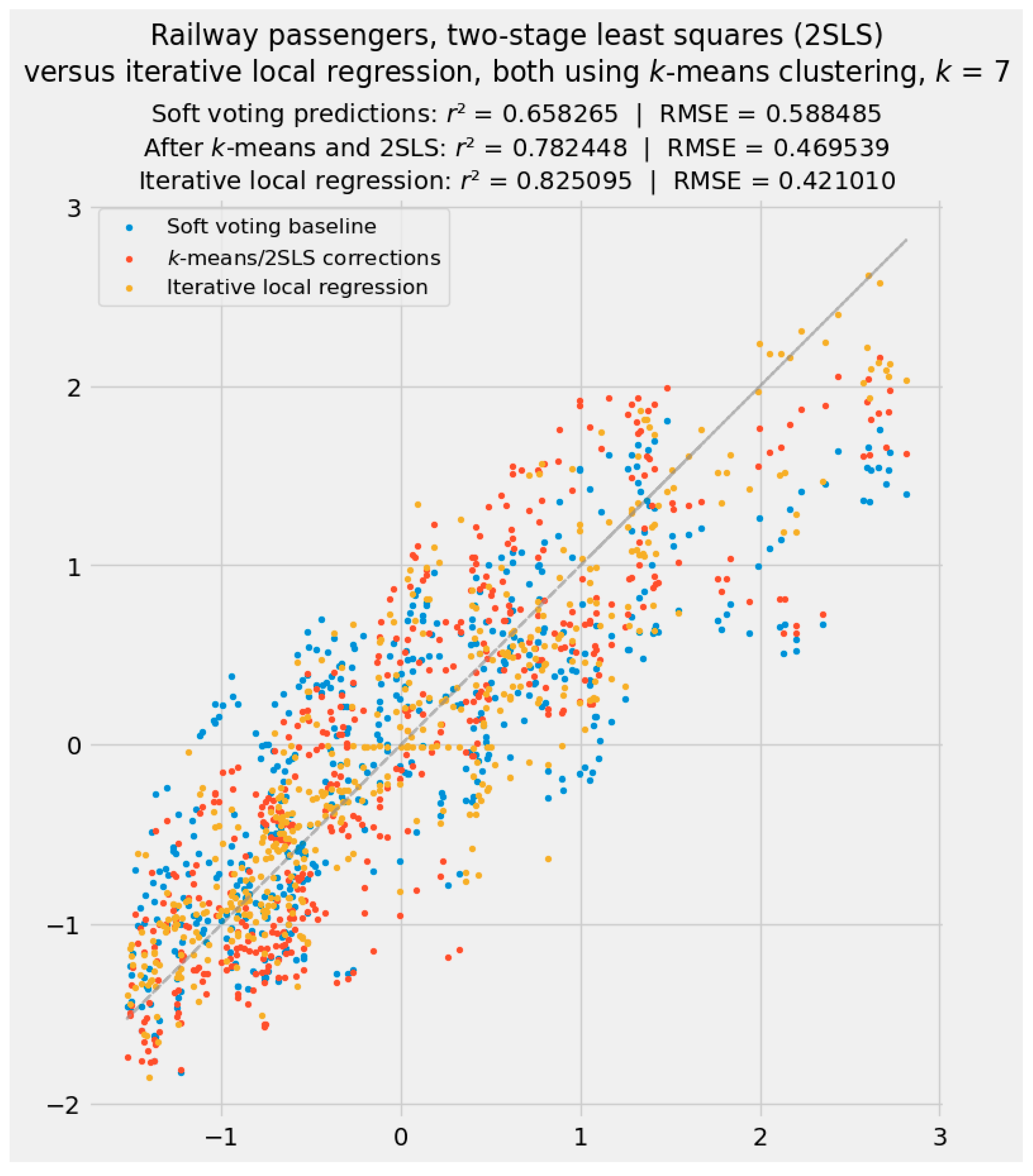
One final method remains for improving predictions. A 2SLS correction within seven clusters yielded results somewhere between 2SLS correction based on fixed geopolitical and time entities and iterative local regression using distance-based k-means clusters (Figure 5). This correction, unlike the 2SLS correction of the unconditional drift term depicted in Part 3, did not rely on stylized “Carolingian distance” or discrete units of time. Instead, 2SLS corrections of residuals for each cluster-based regression proceeded according to each observation’s Euclidean distance from the cluster centroid. Goodness of fit of r² = 0.782448 and RMSE = 0.469539 placed this method above the original 2SLS exercise based on fixed entities. But the corrective effect still trailed that of iterative local regression, despite the application of Ridge (ℓ₂-penalized) regression.

The predictive results depicted in Figure 5 complete the progression. K-means clustering identifies the distinct cohorts where 2SLS and local regression should be applied. In this study, local regression proves superior in improving predictive accuracy. That exercise improves goodness of fit from r² = 0.658265 to 0.825095. Goodness of fit as measured by root mean squared error improves from RMSE = 0.528485 to 0.421010.

5. Discussion and Conclusions

This paper implements two distinct methods for improving panel data estimates: two-stage least squares (2SLS) reevaluation of residuals along one or more dimensions and iterative local regression. Those methods, developed in geospatial econometrics and time-series forecasting, can dramatically improve both predictive accuracy and causal inference in panel data analysis.

Iterative local regression outperforms 2SLS evaluation of residuals from unconditional baseline regression. Although neither method, in principle, has an a priori advantage, the superior performance of iterative local regression is not surprising. In the absence of precise geographic coordinates and a fully connected graph of Haversine distances, the most readily implemented distance metric for 2SLS correction of the drift term was a single vector of stylized “Carolingian distances” from the historical European center of political and cultural gravity at Aachen. The surprising, perhaps even miraculous, effectiveness of this expedient testifies to the galvanizing influence of Charlemagne, even twelve centuries after his death. Future research could overlay this vector of Carolingian distances in a meta-analysis of panel data studies involving EU member-states.

The use of k-means clustering proved decisive. Clustering as a form of preprocessing identifies cohorts where 2SLS and local regression should be applied. A progression culminating in the application of these methods to formally identified clusters—as distinct from intuitive or convenient boundaries based on geopolitical entities—continuously improves goodness of fit.

In addition to improving predictive accuracy in ŷ, the primary goal on the left-hand side of the regression equation, these methods also enhance the search for credible causal inferences on the right-hand side. Cluster centroids and the weighted mean of local regression coefficients provide further insights into causal inferences drawn from generalized linear methods. Meaningful departures, such as the reversal of the sign accompanying a nontrivial coefficient for the fertility variable, undermine designations of statistical significance under the conventions of null hypothesis significance testing.

Absent resort to gray- or black-box methods of machine learning or artificial intelligence, improvements this dramatic are rarely attained in conventional econometrics. Though “machine learning [typically] belongs in the part of the toolbox marked ŷ rather than in the more familiar β compartment” [16] (p. 88), the methods in this paper advance analytical interests on both sides of the regression equation. Readily generalizable to a wide variety of economic studies, they deserve broader application.

References

1. Poufinas, T.; Panagopoulou, A.C.; Chen, J.M. On the economic determinants of railway passenger traffic in the European Union. Atl. Econ. J. 2025; 53, in press. [Google Scholar]
2. Chen, J.M. Drift and diffusion in geospatial econometrics: Implications for panel data and time-series. Comput. Sci. Math. Forum, 2025; in press. [Google Scholar]
3. Chen, J.M. A practical introduction to regularized regression for panel data. Contrib. Stat. 2025; in press. [Google Scholar]
4. Dubin, R.A. Spatial autocorrelation and neighborhood quality. Reg. Sci. Urban Econ. 1992, 22, 433–452. [Google Scholar] [CrossRef]
5. Maydeu-Olivares, A.; Shi, D.; Rosseel, Y. Instrumental variables two-stage least squares (2SLS) vs. maximum likelihood structural equation modeling of causal effects in linear regression models. Struct. Equ. Model. Multidiscip. J. 2019, 26, 876–892. [Google Scholar] [CrossRef]
6. Inoue, A.; Solon, G. Two-sample instrumental variable estimators. Rev. Econ. Stat. 2010, 92, 557–561. [Google Scholar] [CrossRef]
7. Haddock, D.D. Basing-point pricing: Competitive vs. collusive theories. Am. Econ. Rev. 1982, 72, 289–306. Available online: https://www.jstor.org/stable/1831533 (accessed on 28 May 2025).
8. Thisse, J.-F.; Vives, X. Basing point pricing: Competition versus collusion. J. Indus. Econ. 1992, 40, 249–260. [Google Scholar] [CrossRef]
9. Supreme Court of the United States. Federal Trade Commission v. Cement Institute. United States Rep. 1948, 333, 648–740. [Google Scholar]
10. Pace, R.K.; Barry, R. Sparse spatial autoregression. Stat. Prob. Lett. 1997, 33, 291–297. [Google Scholar] [CrossRef]
11. Likas, A.; Vlassis, N.; Verbeek, J.J. The global k-means clustering algorithm. Pattern Recognit. 2003, 36, 451–461. [Google Scholar] [CrossRef]
12. Pham, D.T.; Dimov, S.S.; Nguyen, C.D. Selection of K in K-means clustering. J. Mech. Eng. Sci. 2005, 219, 103–119. [Google Scholar] [CrossRef]
13. Hout, M.C.; Papesh, M.H.; Goldinger, S.D. Multidimensional scaling. WIREs Cogn. Sci. 2013, 4, 93–103. [Google Scholar] [CrossRef] [PubMed]
14. Efron, B.; Hastie, T.; Johnstone, I.; Tibshirani, R. Least angle regression. Annals Stat. 2004, 32, 407–499. [Google Scholar] [CrossRef]
15. Wasserstein, R.L.; Schirm, A.L.; Lazar, N.A. Moving to a world beyond “p < 0.05”. Am. Stat. 2019, 73 (Suppl. 1), 1–19. [Google Scholar] [CrossRef]
16. Mullainathan, S.; Spiess, J. Machine learning: An applied econometric approach. J. Econ. Persp. 2017, 31, 87–106. [Google Scholar] [CrossRef]
Figure 1. Predictive results from the soft-voting aggregation in [1], highlighting the results by country. Traffic in Romania and Ireland is overestimated. Traffic in Hungary, Austria, and France is underestimated.
Csmf 11 00031 g001
Figure 2. Two-stage least squares corrections to residuals based on “Carolingian distances” from Aachen to all 25 capital cities and on the 19 years in the dataset.
Csmf 11 00031 g002
Figure 3. The k-means clustering of European railway passenger traffic, k = 7, as projected onto three dimensions through multidimensional scaling.
Csmf 11 00031 g003
Figure 4. Fitted values from an aggregation of iterative local regression after k-means clustering. Each cluster, in a distinct color, displays its own regression line. Four of the countries displaying the worst estimates in Figure 1 (Romania, Ireland, Austria, and France) no longer appear as outliers.
Csmf 11 00031 g004
Figure 5. A summary of fitted values from 2SLS correction and iterative local regression after k-means clustering. Among the methods applied in this article, cluster-based iterative local regression provided the greatest improvement in predictive accuracy.
Csmf 11 00031 g005