Abstract
This study examines the synchronization of economic and growth cycles between China and the United States of America amid ongoing economic and geopolitical tensions. Using a Markov-Switching–Vector Autoregression (MS-VAR) model, the analysis applies the Hodrick–Prescott and Baxter–King filters to monthly data from January 2000 to December 2024, capturing trends and cyclical fluctuations. The findings reveal asymmetries in economic synchronization, with differences in recession and expansion durations influenced by trade disputes, financial integration, and external shocks. As the rivalry between the two nations intensifies, marked by trade wars, technological competition, and geopolitical conflicts, understanding their economic co-movement becomes crucial. This study contributes to the literature by providing empirical insights into their evolving interdependence and offers policy recommendations for mitigating asymmetric shocks and promoting global economic stability.
1. Introduction
The economic relationship between China and the United States of America (USA) forms a cornerstone of global economic dynamics, profoundly influencing trade, investment, and financial flows. As the world’s two largest economies, their interactions extend beyond bilateral relations to shape global markets, economic stability, and growth. Despite this interdependence, structural differences, policy divergences, and geopolitical tensions between China and the USA create complexities, underscoring the importance of analyzing their economic synchronization trends.
This study focuses on synchronizing economic and growth cycles between China and the USA, two of the world’s largest economies. Given their dominant roles in global trade, investment flows, and financial markets, any divergence or alignment in their economic cycles can have profound implications for international stability and policy coordination. Understanding the degree of synchronization between these two economies is essential for forecasting global trends and designing coordinated macroeconomic policies, especially in light of events such as the 2008 global financial crisis and recent USA–China trade tensions.
Trade integration between China and the USA has expanded significantly since the 1990s, reshaping their economies and global trade patterns. USA imports from China rose from 3.1% of total imports in 1990 to 19.2% in 2020, while USA exports to China increased from 1.3% to 9.3% during the same period. By 2006, China had become the USA’s second-largest trade partner, overtaking Mexico. Similarly, China’s exports to the USA grew from 8.3% to 17.5% of its total exports between 1990 and 2020 [1].
The USA and China are investing significantly in smart infrastructure (SI) to address growing energy, transportation, and housing demands by integrating information and communication technology with physical infrastructure [2]. In the USA, the Biden administration introduced a USD 2.3 trillion infrastructure modernization plan in 2021, slated for implementation over eight years, with a strong emphasis on clean energy, semiconductors, and smart grids. Similarly, China launched a USD 2.1 trillion SI investment initiative in 2020 to accelerate post-pandemic recovery, contributing to improved living standards [3]. China’s extensive digital ecosystem, supported by over 1.011 billion internet users in 2021 and 511 million active Sina Weibo users, facilitates spatial–temporal analysis of public preferences, offering valuable insights for optimizing resource allocation and development priorities according to the China Internet Network Information Center in 2021. While China leverages its vast digital infrastructure to enhance policy efficiency, the USA prioritizes data-driven approaches to modernizing its infrastructure and improving resource management.
The issue of whether more Foreign Direct Investment (FDI) will lead to stronger or weaker business-cycle connections remains unclear in light of China’s relatively strict capital regulations. This channel may not be as crucial for China’s and India’s business cycles, as they specialize vertically in international trade. As ref. [4] points out, the rising Asian superpowers and their trading partners may experience business-cycle divergence if specialization forces prevail. Changes like China’s 2001 accession to the WTO, accelerating its integration into the global economy, and reducing trade barriers, were catalysts for these shifts. Concurrently, China’s rapid growth in manufacturing productivity during the 1990s and 2000s enabled it to dominate global markets. Numerous studies [5,6] have demonstrated that the expansion, commonly referred to as the “China shock,” significantly impacted job opportunities, wages, and prices in the USA manufacturing sector. This has led to trade wars, particularly during the Trump administration, which imposed tariffs on Chinese goods to address the trade imbalance. Beyond economic disputes, the two nations are engaged in a broader geopolitical rivalry, particularly in the Indo-Pacific region. China’s expanding military presence and assertive foreign policies, such as the Belt and Road Initiative, challenge the USA’s strategic interests.
Human rights concerns have further strained relations, with the USA criticizing China’s treatment of ethnic minorities in Xinjiang and its policies in Hong Kong as violations of international norms. Additionally, tensions are exacerbated by disagreements over global governance, cybersecurity, military security, and climate change, creating a complex and often confrontational relationship.
Despite these conflicts, both nations recognize the need for cooperation on global challenges. The USA and China have collaborated on clean-energy transitions as the world’s largest greenhouse gas emitters. During COP26 in 2021, they signed a joint declaration on climate cooperation, reaffirming their shared responsibility in addressing environmental issues [7]. According to [8,9], the frameworks most likely to replace engagement are strategic competition, competitive coexistence, and containment, similar to those employed during the Cold War.
It would take the USA a decade to reach any of these frameworks, and for each of them, one could devise a convincing story about how and why Washington would achieve it. Given the two countries’ shared interests and the economic and ecological ties that link them, Washington could settle on coexisting competitively after adjusting to a more forceful China. On the other hand, strategic competition is likely to remain in place as it sidesteps the alternatives’ hostile policy and political effects.
Nevertheless, until a Cold War-style framework, which is not unattractive to Americans who recall defeating the Soviet Union, takes hold, bilateral ties are likely to continue deteriorating. Different USA attitudes toward China would result from these plausible paths. It is essential to avoid fatalism in USA–China relations, and the fact that both options seem conceivable should give stakeholders and policymakers the freedom to choose the future they desire after the interaction. Those who prioritize reducing the likelihood of a hot or cold conflict while maintaining room for cooperation (without reverting to engagement) can find a path forward within a framework of competitive coexistence.
“Competition without conflict” has become the new normal, but it does not mean engagement is returning. Nonetheless, the USA and China should be commended for preventing severe adverse outcomes, such as complete decoupling and armed confrontation. However, there is no assurance in the relations’ long-term structural elements or short-term motivations. To continue moving forward in 2024, we must take several national, bilateral, and international measures.
First and foremost, we must all work together to prevent a worsening of tensions and a full-scale war in the South China Sea and Taiwan Strait. Despite the uncertainty surrounding the Taiwanese election, it is clear that both sides will need to exercise caution once the results are announced. We must also remain vigilant during the May inauguration of Taiwan’s new leader and their early months in office. Finding a solution to the tense situation between China and the Philippines over the Second Thomas Shoal, especially in light of Beijing’s increasingly aggressive actions, is no easy feat.
Next, with new avenues of communication now open, the USA and China must proceed with consultations across all domains, including trade, technology, AI, climate, and security. The dialogue will be fruitful in and of itself, especially considering the prior lack of communication. However, it is reasonable to anticipate that the USA and China will soon refine their agenda in their respective working groups, transitioning from consultations to negotiations, yielding solid outcomes.
China’s economy has generally experienced a slowdown in traditional growth drivers, such as real estate and investment, alongside rising challenges like demographic imbalances and external pressures from decoupling strategies. Simultaneously, despite persistent inflation and financial tightening, the USA has maintained relatively robust economic growth fueled by private consumption, investment, and targeted fiscal policies. These contrasting trajectories raise essential questions about the degree and mechanisms of growth-cycle synchronization between these two nations.
Economic-cycle synchronization between major economies has long been a subject of academic interest due to its implications for global trade, financial stability, and policy coordination. While trade intensity and financial integration are often cited as primary drivers of synchronization, recent studies suggest that structural changes, sectoral specialization, and geopolitical shifts also play significant roles. We can refer to [10]’s study as an example to support this idea. The findings suggest that exchange-rate regimes have a bidirectional impact on synchronizing economic cycles between advanced and emerging economies. While this effect is positive in the short term, it gradually diminishes and eventually turns negative in the medium term.
In today’s profoundly interconnected global economy, it is imperative to comprehend the synchronization of economic and growth dynamics between China and the USA. These two countries are the world’s largest economies and account for a significant proportion of global trade, investment, and technological advancement. Any economic fluctuation in either country, whether driven by trade tensions, changes in monetary policy, or external shocks such as pandemics, can generate significant spillover effects across the global economy. Ongoing geopolitical shifts and structural changes to global supply chains further highlight the need to examine how synchronized their business cycles have become. This paper addresses this crucial issue by applying a non-linear Markov-Switching–Vector Autoregression (VAR) model to capture the time-varying nature of their economic co-movements. The findings are highly relevant for policymakers, investors, and international institutions seeking to anticipate economic turning points and improve the coordination of macroeconomic policies between major economies.
So, this study aims to fill this gap by employing a Markov-Switching–Vector Autoregression (MS-VAR) model, as proposed by [11], to analyze the synchronization of economic and growth cycles between the two selected countries, China and the USA, using the HP and BK filters from January 2000 to December 2024. The [12] approach is better for identifying economic fluctuations, especially peaks and troughs. By integrating a trend and cycle approach, the study provides a comprehensive framework for disentangling long-term growth trends from short-term cyclical fluctuations. This methodological advance is crucial for capturing regime shifts and non-linear dynamics that traditional models may miss.
This is why we have settled on this timeframe (M1-2000 to M12-2024): The economic, geopolitical, and ideological divides between China and the USA have escalated their relationship into a full-blown conflict. The USA continues accusing China of unfair trade practices, including currency manipulation, forced technology transfers, and intellectual property theft, escalating the trade dispute. Tensions persist, particularly in geopolitics and technology, despite growing economic interdependence. The USA’s armaments shipments and Taiwan and China’s territorial claim challenges are two major geopolitical flashpoints in the South China Sea dispute [13]. The USA’s export limitations on semiconductors and concerns about cybersecurity have ratcheted up the technological rivalry. Conversely, China is making significant efforts to solidify its dominance in key technological domains [14].
The research question is as follows: To what extent does the synchronization of economic and growth cycles between China and the USA reflect the dynamics of trade dependence and rivalry, particularly regarding technological competition and comparative advantage?
It is for this reason that the contributions of this paper are threefold. First, it offers a novel application of the MS-VAR model to examine economic and growth synchronization, capturing asymmetries and regime-specific interactions. The Markov-switching model has also been used to analyze business-cycle synchronization in Asia, notably by [15], who show common negative growth patterns between the emerging economies of China and India. These results underscore the significance of robust trade and financial ties with advanced economies, particularly during periods of crisis, such as the COVID-19 pandemic. Second, it bridges the gap in the literature by focusing on the dual role of structural transformations and external shocks in shaping bilateral synchronization. Ultimately, the study offers policy insights into the implications of synchronization for global economic governance, highlighting the necessity of coordinated strategies to mitigate asymmetric shocks.
The evolving economic, technological, and geopolitical interactions between China and the USA underscore their pivotal roles in shaping global trends. While their approaches to development differ, their investments in smart infrastructure and their interdependence in trade highlight the critical importance of fostering sustainable collaboration to address shared challenges and drive global economic growth.
2. Literature Review and Theoretical Background
Though marked by rivalry, economic synchronization between the USA and China is evident in their interconnected markets and supply chains. Economic policies, shifts in trade, and technological advancements in one country often have ripple effects in other countries, highlighting the deep interdependence. Despite periods of tension, such as trade disputes and technological competition, the synchronization of their economic cycles remains a key factor in shaping global growth trends. Any significant policy shift in one of these economies can significantly affect the other, with broad implications for international markets.
Much discussion has centered on the Optimal Currency Areas (OCAs) theory and the relationship between international trade and business-cycle synchronization. Previous research by [16,17,18] established that monetary unions can only succeed if trade integration and cycle synchronization are in place. As ref. [19] pointed out, economic integration through trade links promotes business-cycle synchronization by serving as a conduit for transmitting shocks between nations.
In the Asian context, the Chinese and Japanese cycles correlate little with those of other Asian countries [20]. Furthermore, research by [21] reveals that value-added trade increases synchronization, while exchange-rate volatility has the opposite effect. The Markov-switching model has also been used to analyze business-cycle synchronization in Asia, notably by [15], who show common negative growth patterns between the emerging economies of China and India. These results underscore the significance of robust trade and financial ties with advanced economies, particularly during periods of crisis, such as the COVID-19 pandemic.
Additionally, several studies have investigated the correlation between business cycles in East Asia. For example, ref. [22] finds standard business cycles for the East Asian region. Moreover, ref. [23] finds that trade integration (and, to a much lesser degree, financial integration) enhances output co-movement in East Asia. Ref. [24] finds that increasing the share of electronic products in foreign trade increases the correlation of business cycles for countries around the Pacific. Also, refs. [25,26,27] find that trade is an essential determinant of business-cycle correlation for East Asian countries.
In their study on the similarity of external adjustments among Asian economies, ref. [28] highlight that business cycles have decoupled between the OECD countries, China, and other emerging Asian economies. Ref. [29] examine the dwindling role of the USA in Asia. Ref. [30] find that business cycles have converged within the OECD and emerging markets, including non-Asian countries.
However, this relationship is not unequivocal. Ref. [31] shows that the intensity of trade links between two countries increases the correlation of their output changes. Conversely, ref. [4] argues that increased integration allows for specialization, which can generate asymmetric sectoral shocks, thereby reducing the synchronization of economic cycles. This ambivalence is reflected in empirical studies, where some authors, such as [32], demonstrate that countries with intensive trade exhibit greater output co-movement, while others, like [33], emphasize the importance of intra-sectoral trade.
Financial integration also plays a significant role. Ref. [34] demonstrate that economic integration can reduce cycle synchronization due to the increased specialization it fosters. However, ref. [35] highlights a positive correlation between economic integration and cycle synchronization. Studies of financial crises suggest that capital flows become increasingly synchronized, particularly in Asia [36,37,38].
For the USA, studies of business cycles at the state level reveal significant variation in recession and expansion phases, suggesting that cycle synchronization may be influenced by regional factors such as industrial diversification and fiscal policies [39,40,41]. Wavelet analysis, as shown by [42], also reveals that the business cycles of USA states are highly synchronized, with a significant influence of distance on synchronization, confirming gravity mechanisms in trade.
Several studies have examined the synchronization of business cycles and financial markets, providing valuable insights into understanding the economic interdependence between significant economies. Ref. [43] employed wavelet analysis to investigate the co-movement of business cycles across various time horizons, highlighting the significance of frequency-based synchronization in global markets. Ref. [44] explored the relationship between financial markets and macroeconomic aggregates, highlighting the role of financial linkages in driving business-cycle synchronization. Ref. [45] further analyzed the transmission of macroeconomic shocks across countries, emphasizing the influence of trade and financial integration on co-movements of business cycles. These studies are particularly relevant in the USA-China economic relations, as trade disputes, financial interdependence, and external shocks continue to shape the synchronization of their economic cycles [15]. By building on this literature, the present study seeks to deepen the understanding of how economic fluctuations in China and the USA interact, considering the impact of trade, financial markets, and external shocks on their business-cycle alignment.
The synchronization of economic cycles and growth between the USA and China has not been extensively studied despite the critical importance of the USA–China relationship in today’s global economy. This gap in the literature underscores the need for research that focuses on understanding how these two significant economies interact and synchronize their economic activities.
Building on the insights from the literature review, two hypotheses can be proposed to analyze the dynamics of economic synchronization between China and the USA. These hypotheses aim to explore the nature of the economic relationship between the two nations, assessing whether China is increasingly aligning its economic cycles with those of the USA or if the USA is adapting to China’s economic trajectory.
The first hypothesis posits that China and the USA are experiencing similar economic growth and cycles, leading to a balanced synchronization of their economic activities. This parity suggests that both nations are equally influenced by global economic trends, resulting in aligned business cycles.
(H1):
Synchronization of the USA and Chinese economic and business cycles.
The second hypothesis asserts that the USA is ahead in economic development and growth cycles compared to China. It suggests that the USA’s economic policies and innovations set the pace for global economic trends, thereby influencing China’s economic trajectory and leading to a lag in synchronization.
(H2):
China’s economic and business cycles lag behind those of the USA.
3. Methodology
3.1. The Model General Framework
There are multiple ways to view the business cycle, and according to [46], each approach has distinct turning points. However, the New Neoclassical Synthesis and studies of actual cycles have cast doubt on this method ([46,47,48,49]). The most recent piece of writing that has been published, titled “Growth Cycles,” instead alludes to the business cycle as defined by [50] as “the movement of GDP relative to its trend.” To further dissect macroeconomic data into trend and cyclical components, real business-cycle theorists also employed specialized statistical methods, including the [51] filter, the band-pass filters proposed by [52], and subsequently refined by [53]. The statistical analysis introduced by the fundamental cycle theory was based on the (HP) filter. However, economic policymakers consider the immediate and distant future when making decisions. According to their findings, Euro-Mediterranean commerce does not significantly impact the integration of Central European nations. They also reasoned that the southern Mediterranean countries’ failure to keep up with European market demands was to blame for their sluggish progress. The export of textiles to the European Union is where the two groups compete the most fiercely.
Given the nature of our research and the objectives set, this study also presents the tests of unit roots with ruptures, such as [54,55], as well as the techniques of [56,57] for the detection of cyclic asymmetry. Nonetheless, it is worth considering the passage on the method of filtering, mainly the (HP) and (BK) filters, which were applied to decompose the time series into trend and cycle components.
The data used are based on monthly observations from January 2000 to December 2024. Due to the narrow time series, we use monthly rather than quarterly data to achieve more observation points (284 observations in our case). All time-series variables were collected from the National Bureau of Statistics. Nearly all empirical research involving developing countries follows this approach due to the short periods inherent in such an assessment. In addition, ref. [58] demonstrate that the conclusions drawn from quarterly data are consistent with those derived from monthly data.
To understand the contribution of the various impulses to economic fluctuations in the USA and China, we have included a series of domestic and external variables in our model, namely the industrial production index (IPI) and the consumer price index (CPI). This series of variables is expressed in logarithms. IPIR represents the seasonally adjusted industrial production index, calculated using the Census X11 method in EViews 12.0 and normalized by the consumer price index. Specifically, IPIR is defined as IPI_S/CPI_S, where IPI_S is the seasonally adjusted industrial production index, and CPI_S is the seasonally adjusted consumer price index.
Figure 1 and Figure 2 show the monthly dynamics of industrial production (IPIR) for China and the USA, filtered according to the Hodrick–Prescott (HP) and the Baxter–King (BK) methods, respectively. We can directly read their relative variance and co-movements by superimposing the series on the same time axis.
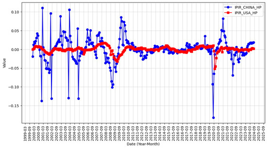
Figure 1.
HP-filtered cyclical components of industrial production in the USA and China.
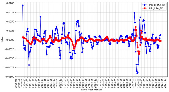
Figure 2.
BK-filtered cyclical components of industrial production in the USA and China.
The first figure (HP) reveals markedly greater volatility in the Chinese series, particularly before 2010. This reflects a phase of rapid structural transformation characterized by frequent adjustments in economic policy. By contrast, the USA series appears more stable and regular. However, the two economies experience simultaneous and converging shocks during major crises such as the 2008 financial crisis and the COVID-19 pandemic, reflecting growing interdependence.
The second figure (BK), isolating short- and medium-term cyclical components, confirms this trend towards synchronization since 2010, while revealing occasional phases of decorrelation. The observed economic responses to recent exogenous shocks, notably post-2019, show a more marked correlation, supporting the hypothesis of a stronger cyclical coupling. These visual elements, now presented comparatively on the same temporal basis, support and complement the empirical findings of the MS-VAR model, which identifies regimes alternating between strong and weak synchronization.
3.2. Hamilton’s Approach (1989)
Markov-Switching–Vector Autoregressions (MS-VAR) can be seen as an extension of the finite-order basic VAR model with an order denoted as p. Let us contemplate a p-order autoregression applied to a time-series vector in multiple dimensions k, :
where , and are fixed. Denote as the dimensional-shift polynomial , we assume that there are no roots on or inside the unit circle pour , where “L” is the shift operator, so that .
If a normal distribution of the error is assumed, , (Equation (1)) is recognized as the stable Gaussian VAR(p) model in its intercept form. It can also be seen as the form representing the fitted mean of a VAR model (Equation (2)):
is the dimensional average of , where . Because its parameters are time-invariant, the stable VAR model is not always the best choice when working with time series that might experience regime shifts. However, a more all-encompassing approach to regime switching is the MS-VAR model. An unobservable regime variable , representing the likelihood of being in a particular state of the world, is the essential notion behind this class of models. The parameters that govern the data creation process of the observed time-series vector depend on this variable. If we want to deduce regime transitions from data, we need to build a model to generate the regimes. The Markov-switching model is unique because it is based on the assumption that the unobservable state is defined by transition probabilities as a discrete-time, discrete-state Markov stochastic process (Equation (3)).
With greater precision, we proceed under the assumption of an irreducible ergodic Markov process denoted as “M,” characterized by a transition matrix (P) (Equation (4)):
where for .
The ergodicity and irreducibility assumptions are fundamental for the theoretical properties of MS-VAR models; for a complete description of the Markov chain theory as applied to Markov-switching models, see [11]. The estimating procedures given in [59] are sufficiently general to handle these degenerate cases; for example, when there is a single model or when the absorbing state is interrupted by a single jump (structural break), that remains until the end of the observation period. Markov-Switching–Vector Autoregressions of order p and M schemes are considered (Equation (5)) as a generalization of the mean-fit VAR(p) model in (Equation (2)):
where and are shift functions of the parameters describing the dependence of the parameters on the realized plan , for example:
In Equation (6), an abrupt shift in the process occurs due to a regime change. However, there are cases where it is more reasonable to assume that the mean gradually converges to a new level after transitioning from one regime to another. In such cases, a model with a regime-dependent intercept term can be used:
The mean-fitted form of Equation (4) and the intercept form of Equation (7) of an MS(M)-VAR(p) model are not similar, unlike the linear VAR model. As [59] demonstrated, these shapes suggest distinct dynamic changes in the measured variables after a regime shift. The observed time-series vector will immediately jump to its new level if the mean, denoted by , undergoes a gradual shift. The dynamic reaction to a single regime shift in the intercept term is analogous to a shock of the same kind in the white-noise series, on the other hand. A model where some parameters are state-dependent and others are constant might be more suitable for practical applications of the Markov chain. Maximum Likelihood and Hamilton’s non-linear filtering technique are well-established methods for estimating model parameters across regimes introduced and developed by [11]. The need for specialized (MS-VAR) models arises when the error term displays heteroscedastic or homoscedastic behavior or when the autoregressive parameters, means, or intercepts differ across regimes.
3.3. Bry and Boschan’s Approach (1971)
The algorithm of [12] as coded by [60] seeks to detect turning points in business cycles. The turning points occur locally (with an environment of 15 months). At the extreme points of the series, we have:
Other than these two conditions, the identified turning points must verify other restrictions: (1) The troughs and peaks must alternate; (2) peaks must be higher than their adjacent troughs; otherwise, the trough is suppressed; (3) the duration of a complete cycle (separating a peak from a peak or a trough from a trough) must be at least 15 months; otherwise, candidate turning points are deleted; (4) the first turning point in both limits of the series must be more extreme than the endpoint itself (i.e., a trough must be lower than the first point in the series, and a peak must be higher than the last point in the series); otherwise, the turning point is excluded; (5) the duration of a complete phase (which separates a peak from a trough or a trough from a peak) must be greater than 6 months; otherwise, the turning point is removed; (6) the first and last quarters do not include turning points (they do not have enough points preceding or succeeding them in this position).
The main advantage of non-parametric methods is the simplicity of their rules. The non-parametric assumptions are not very restrictive regarding the underlying data, except that for some observations to be classified, they must not be at the extreme of the sample.
The results of nonparametric dating are robust and insensitive to changes in sample size, allowing them to be compared across different databases. On the other hand, the merits of nonparametric methods, including their simplicity and non-specificity, have generated criticism.
4. Estimation and Interpretations
This section presents the core empirical analysis of the study, focusing on the synchronization of economic and growth cycles between China and the United States of America (USA). The section details cycle extraction and decomposition using the Hodrick–Prescott (HP) and the Baxter–King (BK) filters to identify turning points and cyclical phases. This is followed by applying the Markov-Switching–Vector Autoregression (MS-VAR) model, which captures the regime-dependent behavior of the two economies over time. The findings are synthesized to evaluate the extent of synchronization and draw key policy-relevant insights. This structured approach allows for a comprehensive understanding of the dynamic characteristics of each economy and its bilateral interactions across different regimes. Several seminal studies on cyclical synchronization analysis, including the recent works of [61,62], have addressed the problem of aligning economic cycles.
4.1. Description of Variables

Table 1.
Descriptive statistics of HP and BK filters.
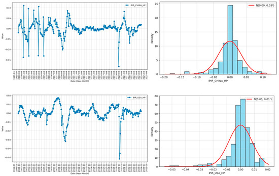
Figure 3.
HP evolution and histogram of filters.
For China, the evolution of the HP filter between January 2000 and December 2024 is characterized by a zero mean with a standard deviation of approximately 0.001. All values are between −0.181 and 0.110. The sample distribution is slightly spread to the right (skewness = −1.018). However, it is strongly leptokurtic (kurtosis = 8.568).
The HP filter correlograms exhibit strong autocorrelation, as indicated by Ljung–Box test probabilities below 5%, which rejects the null hypothesis of no autocorrelation. The Jarque–Bera test also rejects the null hypothesis of normality with a p-value of 0.000. The evolution of the HP filter for the USA between January 2000 and December 2024 is characterized by a zero mean with a standard deviation of approximately 0.000. All values are between −0.051 and 0.017. The series’ distribution is also asymmetric and skewed to the left (skewness = −1.934). However, it is strongly leptokurtic (kurtosis = 10.953).
Now, let us proceed to the descriptive and graphical presentation of the evolution of the different BK filters using Table 1 and Figure 4. A mean of −3.05 × 10⁻⁵ characterizes the BK filter with a standard deviation of −5.36 × 10⁻⁵ between January 2000 and December 2024. All values lie between −0.009 and 0.009. The distribution of the 284 samples is slightly skewed to the right, with a skewness of −0.118. However, it is strongly leptokurtic (kurtosis = 5.501).
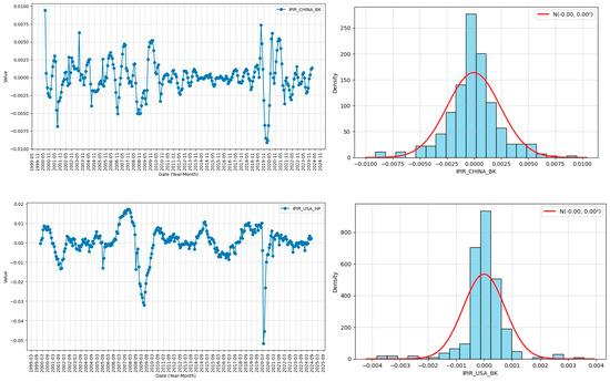
Figure 4.
BK evolution and histogram of filters.
The evolution of the BK filter for the USA between January 2000 and December 2024 is characterized by a mean of −3.81 × 10⁻⁶ with a standard deviation of approximately 1.98 × 10⁻⁵. All values fall within the range of −0.004 to 0.004. In addition, the series’ distribution is asymmetric and skewed to the left (skewness = −0.901). However, it is strongly leptokurtic (kurtosis = 12.387).
The BK filter correlograms indicate a strong presence of autocorrelation, as evidenced by the Ljung–Box test probabilities, all below 5%. This result leads to the rejection of the null hypothesis of no autocorrelation. Additionally, all distributions fail to meet the normality assumption, as the Jarque–Bera test yields a p-value of 0.000, consistently rejecting the null hypothesis at the 5% significance level.
We present the results of the [54,55] tests on all series for the two filters (HP and BK) to check for structural breaks in the following sections. The results of Zivot and Andrews’s unit root tests in Table 2, incorporating the Hodrick–Prescott (HP) and the Baxter–King (BK) filters, highlight distinct USA and Chinese IPIR series dynamics. For the IPIR_USA, the two filters confirm stationarity across the three models, with structural breaks corresponding to significant economic periods, notably in July 2009 and September 2020, and time lags varying according to the filter used. In contrast, IPIR_CHINA yields mixed results under the HP filter, indicating non-stationarity in some models (p-value > 0.05), whereas the HP filter confirms stationarity in all cases, with breaks primarily located around the global financial crisis of 2008–2009. These observations underscore the significance of the methodology employed to capture structural changes and the dynamics of economic time series.
Table 2.
Results of the Zivot & Andrews (2002) [54] test at the level.
The results of the unit root tests, presented in Table 3, using the Hodrick–Prescott (HP) and Baxter–King (BK) filters, reveal distinct dynamics for the USA and IPIR_CHINA series.
Table 3.
Results of the Perron (1997) [63] test at the level.
Using the HP filter, the stationarity of the IPIR_USA cannot be confirmed, as the t-statistics are low and close to the critical thresholds. This is despite identifying significant structural breaks, notably in 2011M09, 2012M09, and 2019M05, corresponding to periods marked by considerable economic changes.
On the other hand, for IPIR_CHINA, the t-statistics are significantly more robust, indicating likely stationarity, with notable structural breaks such as 2020M03 (the onset of the COVID-19 pandemic) and 2006M12 (the global financial pre-crisis).
The BK filter confirms stationarity for both series, with highly significant t-statistics and structural breaks associated with global economic shocks, including the global financial crisis, the COVID-19 pandemic, and trade tensions. These results underscore the importance of the BK filter in capturing the underlying dynamics and exogenous shocks that affect the series studied.
The [55] model, presented in Table 4, extends traditional unit root tests by incorporating the hypothesis of structural breaks in time series. Unlike traditional tests, which assume stationarity around an invariant linear trend, Pappel’s model enables the identification and testing of breakpoints that are likely to affect the dynamics of economic variables.
Table 4.
Results of the Lumsdaine & Papell (1997) [55] test of BK and HP filters.
This approach provides a deeper understanding of economic series by taking into account significant shocks, such as financial crises or structural reforms, which can significantly impact the behavior of the studied series.
The IPIR_HP series remains non-stationary for the USA in all models, suggesting that shocks have persistent effects and do not return to a long-term trend. On the other hand, the IPIR_BK series exhibits stationarity in models A and C, indicating its capacity to absorb shocks following structural disruptions, notably those associated with the 2008 financial crisis.
For China, the results indicate partial stationarity for the IPIR_HP and IPIR_BK series, particularly in models A and C, suggesting resilience to economic disturbances. These differences underline the importance of structural breaks and methodological specifications in analyzing economic dynamics while highlighting the need for tailored approaches to managing economic imbalances.
Table 5 presents the results of the Brock–Dechert–Scheinkman (BDS) test applied to the IPIR series for China and the USA after applying the Hodrick–Prescott (HP) filter. These results confirm the presence of significant non-linear behavior.
Table 5.
BDS test results for HP and BK filters.
The BDS statistics increase systematically with the order of integration (m) for both series, with values ranging from 0.106 to 0.221 for China and 0.145 to 0.353 for the USA. The associated probabilities (p-value = 0.000) indicate a rejection of the null hypothesis of independence, highlighting complex dependencies and persistent non-linear patterns.
The higher magnitude of the BDS statistics for the USA suggests a more pronounced non-linearity compared to China, reflecting structural differences in the two countries’ economic dynamics.
These results highlight the limitations of the HP filter in eliminating these dependencies and justify the use of non-linear models to analyze these series, thereby more effectively capturing the underlying dynamic interactions.
The presence of significant non-linear dependencies is confirmed by the results of the BDS test in Table 5 applied to the IPIR series for China and the USA after Baxter–King (BK) filtering. The BDS statistics systematically increase with the order of integration (m), ranging from 0.112 to 0.247 for China and 0.145 to 0.329 for the USA. The associated probabilities (p = 0.000) systematically reject the null hypothesis of independence. These results indicate that the series exhibits a complex dynamic behavior incompatible with a purely linear or random process.
In addition, the higher values observed for the USA indicate more pronounced non-linear dependencies, which may reflect structural or cyclical differences between the two economies. Moreover, these observations show that, although the BK filter is designed to extract specific business cycles, it fails to eliminate these underlying nonlinearities. This justifies using non-linear analytical models to better understand the economic dynamics under study.
4.2. Cycle Presentation and MS-VAR Modeling
The results of the cyclical asymmetry test (see Table 6), applied to the IPIR series for the USA and China, reveal different asymmetric behavior between the two economies after filtering with the HP and BK filters.
Table 6.
Cyclic asymmetry test.
Concerning the HP filter, the triple tests show no significant asymmetry in the business cycles of the two countries, with p-values of 0.295 and 0.810, respectively. However, the Sichel test indicates a significant asymmetry, particularly a strong negative asymmetry for China (skewness = −0.906) and a weaker one for the USA (skewness = −0.119).
This suggests that the business cycles of the two countries are more marked by periods of slowdown, although this asymmetry is more pronounced for China. As for the BK filter, the results show a significant cyclical asymmetry for the USA, with a skewness of −1.049 and a p-value of 0.000, indicating a strong negative asymmetry. For China, the asymmetry is less pronounced (skewness = 1.198), but the lack of significance, according to the Sichel test, indicates that the cycles are relatively symmetrical. These results suggest distinct cyclical dynamics between the USA and China, with more pronounced and asymmetric business cycles in the USA compared to more balanced cycles in China.
The business-cycle results in Table 7, estimated using the [12] method applied to the HP filter, reveal structural differences between the USA and Chinese economies.
Table 7.
Turning points estimated by the Bry & Boschan (1971) [12] method for the HP filter for the USA and China.
An analysis of economic cycles in the USA and China reveals contrasting duration, volatility, and evolution dynamics. In the USA, recessions are longer (19.6 months on average) than expansions (15.9 months), with a higher average cycle length (34.6 months between two troughs).
The USA economy follows a cyclical pattern typical of advanced economies, marked by major financial crises, such as the 2008 recession, which lasted 17 months, and the 2020 recession, linked to the pandemic. These crises are generally followed by recoveries supported by accommodating monetary and fiscal policies. However, recent cycles have shown increasing instability, characterized by shorter growth phases and more frequent recessions.
In China, recessions are shorter, averaging 14 months, and expansions are longer, averaging 20 months, indicating better economic stability. However, the structure of the cycles has changed, with a gradual slowdown since 2010 and increased reliance on domestic consumption. The 2008–2009 crisis was quickly overcome thanks to a vast stimulus plan, whereas the 2020 recession lasted 16 months, comparable to that of the USA, but with a faster recovery. Nevertheless, the recent volatility of cycles suggests a transition toward a model closer to advanced economies, with growing structural challenges linked to property, debt, and trade tensions.
An analysis of economic cycles reveals contrasting dynamics between the USA and China. The USA is experiencing more irregular cycles, with sharp recessions and volatile periods of expansion, while China, although relatively stable, has shown a trend toward economic slowdown since 2015.
The 2008 crisis had a more prolonged impact in the USA, while the 2020 crisis affected China more in terms of the economic cycle. In the future, the USA will face increasing instability, fueled by global uncertainty, geopolitical tensions, and inflationary challenges, making monetary and fiscal policy essential to limit the risks of a prolonged recession. For its part, China is moving towards a more balanced growth model that is less dependent on investment and exports. It faces structural challenges such as the property crisis and demographic aging, which could shorten the expansion phases. Ultimately, these two major economic powers must adjust their policies to stabilize their cycles and prevent prolonged crises in an uncertain global context.
These differences highlight distinct strategies for economic management and adaptation to shocks, with significant implications for stabilization policies and long-term growth trajectories. The growth cycles presented in Table 8, estimated using the method of [12] with the BK filter, highlight distinct dynamics between the USA and China.
Table 8.
Turning points estimated by the Bry & Boschan (1971) [12] method for the BK filter for the USA and China.
In the USA, economic cycles are shorter and more volatile. The average recession duration is 9.5 months, and the average expansion is 18.7 months, reflecting a rapid alternation between phases of slowdown and growth.
The 2008 crisis stands out for its 16-month recession, while the downturn linked to the 2020 pandemic was shorter (6 months) but led to an unstable recovery. China’s cycles are longer, with an average expansion of 14.7 months and a complete cycle of 30.3 months, indicating a historically more stable and resilient economy.
However, the 2014–2020 period saw an exceptional 85-month expansion, followed by a sharp contraction, which could point to structural fragilities related to property and the transition to a more internal growth model. The recent volatility of Chinese cycles suggests a gradual convergence towards dynamics similar to those of advanced economies, characterized by more frequent adjustments in response to economic shocks.
Table 9 presents the BK and HP filter MS-VAR regime-switching model estimation at the lowest AIC values of the industrial production index for the countries in our sample between 2000 and 2024.
Table 9.
Estimation and specification of the parameters of the MS-VAR model for HP and BK filters.
Using the BK and HP filters, the MS(2)-VAR(1) model results for synchronizing economic cycles between the USA and China reveal distinct recession and expansion regimes but with asymmetric dynamics. Both filters identify a longer average duration for recession phases (DM = 3.03 months) than for expansion phases (DM = 1.50 months), reflecting instability in growth periods.
Due to their methodological specificities, the parameters associated with each regime differ slightly between the filters but remain consistent in identifying cycle phases. Statistical tests, particularly the Jarque–Bera test, confirm the non-normality of the residuals, and the convergence test validates the robustness of the estimates.
These results highlight distinct economic cycles between the USA and China, marked by significant regime shifts. The longer duration of recessions than expansions suggests imbalances in the synchronization of the business cycles of the two countries, which may be linked to exogenous shocks or structural differences in their economies. These results also underscore the significance of structural factors and economic interconnections in understanding international economic cycles.
While the HP and BK filters help show economic cycles, they have limitations. They assume linear behavior and cannot detect sudden changes or economic phases. The HP filter may distort the timing of cycles, and the BK filter can miss critical long-term trends.
In contrast, the MS-VAR model can capture shifts between economic regimes, such as expansions and recessions. It reflects real-world changes more accurately, especially in countries like China and the USA, which often face unexpected shocks or policy shifts. Unlike filters, the MS-VAR model finds turning points based on the data and shows how economic conditions evolve. This makes it a more powerful tool for analyzing the synchronized two economies.
Analysis of the MS-VAR model results for the HP and BK filters indicates no perfect synchronization between the USA and Chinese business cycles, thus rejecting hypothesis (H1). The transition coefficients suggest that the USA economy transitions more slowly from one regime to another. At the same time, China alternates more frequently between cycles, implying that China lags behind the USA to some extent, which partially validates this.
The coefficients’ values reveal differences in amplitude between regimes, suggesting a structural mismatch. The transition probability (0.669 for Regime 1 and 0.331 for Regime 2) indicates that the USA economy transitions slowly from one regime to another, whereas China responds more quickly to changes. However, Regime 1’s dominance in terms of persistence indicates that the US may retain a more stable dynamic. This pattern partially supports (H2), suggesting China may lag behind the USA regarding business cycles. In short, the analysis indicates that China follows the USA in the evolution of its economic cycles without reversing the lead–lag dynamic between the two powers.
Figure 5 shows the results of two time series with a BK filter, Residuals 1 and Residuals 2, over 289 months. The graphs show that Residuals 1 exhibits more volatile dynamics, with marked oscillations around the zero mean, indicating that the residuals are not perfectly stationary. This dynamic is characterized by regular oscillations around the mean of zero, suggesting that the residuals are not perfectly stationary.
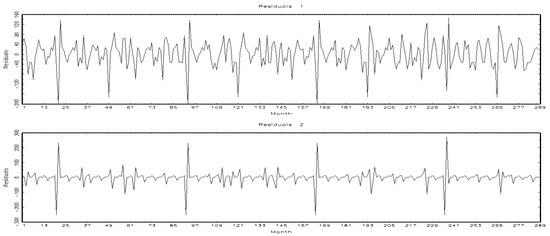
Figure 5.
BK-filtered probabilities with two regimes.
Significant figures indicate periods when exogenous shocks have substantially impacted the series. At the same time, Residuals 2 shows less variability and more damped oscillations. However, both series show similar peaks at regular intervals, suggesting recurring shocks or periodic events. These observations reveal a non-random structure with signs of autocorrelation, necessitating further modeling to capture these irregularities more effectively and enhance the model’s performance.
Figure 6 shows the time series residuals obtained with the HP filter. In the first graph, Residuals 1, we observe significant oscillations around the zero mean with marked variability, indicating more unstable dynamics. The presence of sharp peaks at regular intervals could be the result of recurrent exogenous shocks or disturbances specific to the series. In the second graph, Residuals 2, the variations are more minor around the zero mean, reflecting reduced volatility compared with Residuals 1. However, the peaks observed in Residuals 2 occur at the exact times as those in Residuals 1, suggesting a standard structure or periodic events affecting both series.
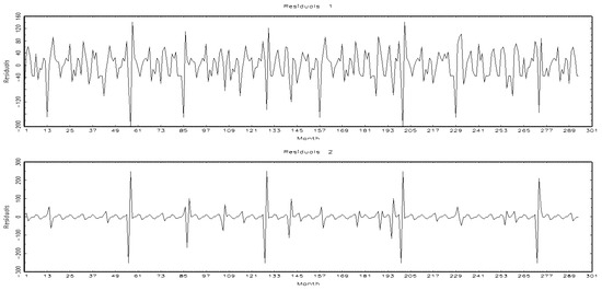
Figure 6.
HP-filtered probabilities with two regimes.
In conclusion, applying the HP filter reveals that the two series share similar shocks but with different amplitudes. Residuals 1 exhibit higher variability, whereas Residuals 2 display smoother dynamics. This indicates partial synchronization of the cycles but with differences in the intensity of the disturbances.
The analysis shows that while China and the USA have experienced fluctuations in business cycles and growth, the timing and intensity of these cycles often differ. The results suggest that full synchronization is limited, especially during global shocks or divergent national policies. However, these findings should be interpreted with caution. Differences in economic structure, policy responses, and external exposure may explain the observed divergences. Therefore, rather than concluding a definitive lack of synchronization, we emphasize that the results point to partial and variable synchronization between the two economies over the period under review.
Figure 5 and Figure 6, which present the filtered and smoothed probabilities and the results in the appendix, clearly indicate that the economic and growth cycles of the three selected countries are significantly out of sync. This desynchronization is reflected in varying time lags or delays between countries during the expansion and recession phases.
The ensuing discussion will be supported by the following illustrative graphic, which encapsulates the results and hypotheses of the present study (Figure 7):
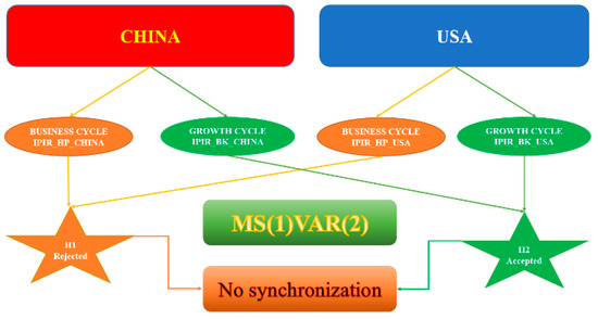
Figure 7.
Graphical illustration.
5. Conclusions and Policy Implications
During this research, we employed the nonparametric procedure of [12] to detect turning points and decompose the classical and growth cycles into cyclical phases. In this way, the non-linear model (MS-VAR) is employed by [11] to highlight the potential lack of synchronization between the economic situations of the two selected regions, China and the USA, from 2000M1 to 2024M12.
Empirical results from parametric and non-parametric approaches confirm a growing synchronization of economic cycles between China and the USA, particularly since the 2000s. Synchronization is a particularly salient phenomenon in the context of global economic shocks, such as the 2008 financial crisis and the 2020 pandemic, thereby underscoring the increasing economic interdependence between the two powers. However, specific periods also reveal partial desynchronization, suggesting that structural differences or divergent economic policies may temporarily weaken this cyclical co-movement.
The Markov-Switching–VAR model, which is based on empirical results, identifies alternating periods of strong and weak economic synchronization. This model has been used to formulate several practical policy recommendations. First, both countries must strengthen macroeconomic dialogue and coordination, particularly during regime shifts or episodes of decoupling. The enhancement of policy communication between central banks has the potential to contribute to stabilizing market expectations and reducing financial volatility. Second, trade and investment policies should be designed with built-in flexibility, allowing timely adjustments in response to evolving synchronization patterns. Thirdly, enhanced transparency in economic data and forecasting practices from both parties would facilitate more accurate assessments of cross-border spillover risks, benefiting global investors and policymakers alike. Finally, regional and international institutions, such as the IMF and the G20, are responsible for promoting joint scenario planning and macroeconomic policy coordination. This is to anticipate and manage the global implications of synchronized downturns or recoveries between these two leading economies.
For more specification, the analysis of the results reveals significant findings regarding the synchronization of economic and growth cycles among the selected countries. The filtered and smoothed probabilities and the residual analysis indicate a lack of synchronization in most selected countries’ economic and growth cycles. This is evident from the observed differences in the timing of peaks and troughs in the cycles.
The graphical analysis suggests that the cycles exhibit noticeable time lags between the countries. These delays underscore that the phases of expansion and recession do not coincide, with a measurable lag that can span several months or periods, depending on the country.
The residuals for the two filters (HP and BK) show differing dynamics. Residuals 1 demonstrates higher volatility with pronounced oscillations, while Residuals 2 exhibits smoother behavior with recurring spikes, indicating structural differences in the cycles.
These results have several important implications for economic policy. First, the high degree of cyclical synchronization between China and the United States of America justifies strengthening bilateral macroeconomic coordination, particularly during times of crisis. Second, policymakers must consider the transmission effect of economic shocks between the two countries when designing fiscal and monetary policies. Third, in the context of heightened trade and geopolitical tensions, a better understanding of cyclical dynamics can help to anticipate the effects of potential economic or strategic disruptions.
In conclusion, the findings confirm the partial synchronization of economic cycles, with significant lags and variations between the selected countries. This highlights the importance of understanding country-specific dynamics and external factors influencing cycle disparities.
Author Contributions
Conceptualization, M.B. and K.H.; methodology, M.B. and M.A.; software, K.H.; validation, H.C., H.B. and M.B.; formal analysis, K.H.; investigation, M.B.; resources, H.C. and M.A.; data curation, M.B.; writing—original draft preparation, M.B. and K.H.; writing—review and editing, M.B. and H.C.; visualization, M.A.; supervision, K.H.; project administration, M.B. and K.H.; funding acquisition, M.B., H.C., and K.H. All authors have read and agreed to the published version of the manuscript.
Funding
This research received no external funding.
Institutional Review Board Statement
Not applicable.
Informed Consent Statement
Not applicable.
Data Availability Statement
The data used are based on monthly observations from January 2000 to December 2024. All time-series variables were collected from the National Bureau of Statistics (NBS) of China (https://www.stats.gov.cn/english/, accessed on 1 February 2025) and FRED (https://fred.stlouisfed.org/, accessed on 1 March 2025). The data presented in this study are available upon request from the corresponding author.
Conflicts of Interest
The authors declare no conflict of interest.
References
- Caliendo, L.; Parro, F. Trade policy. Handb. Int. Econ. 2022, 5, 219–295. [Google Scholar] [CrossRef]
- Huang, G.; Li, D.; Zhou, S.; Ng, S.T.; Wang, W.; Wang, L. Public opinion on smart infrastructure in China: Evidence from social media. Util. Policy 2025, 93, 101886. [Google Scholar] [CrossRef]
- Zhang, J.; Zhang, D.; Li, L.; Zeng, H. Regional impact and spillover effect of public infrastructure investment: An empirical study in the Yangtze River Delta, China. Growth Change 2020, 51, 1749–1765. [Google Scholar] [CrossRef]
- Krugman, P.R. On the Relationship Between Trade Theory and Location Theory. Rev. Int. Econ. 1993, 1, 110–122. [Google Scholar] [CrossRef]
- Adamopoulos, T.; Brandt, L.; Leight, J.; Restuccia, D. Misallocation, Selection, and Productivity: A Quantitative Analysis With Panel Data From China. Econometrica 2022, 90, 1261–1282. [Google Scholar] [CrossRef]
- Brandt, L.; Morrow, P.M. Tariffs and the Organization of Trade in China. J. Int. Econ. 2017, 104, 85–103. [Google Scholar] [CrossRef]
- Blackwill, R.D.; Campbell, K.M. Xi Jinping on the Global Stage: Chinese Foreign Policy Under a Powerful but Exposed Leader; Council on Foreign Relations Press: New York, NY, USA, 2016. [Google Scholar]
- Chivvis, C.S.; Cuéllar, M.-F.; Medeiros, E.S.; Walt, S.M.; Culver, J.; Foot, R.; Bergsten, C.F.; Campanella, E.; Rithmire, M.; Fravel, M.T.; et al. US-China Relations for the 2030s: Toward a Realistic Scenario for Coexistence; Carnegie Endowment for International Peace: Washington, DC, USA, 2024. [Google Scholar]
- Lynch, T.F. The Future of Great Power Competition. In The Routledge Handbook of Great Power Competition; Routledge: London, UK, 2024; pp. 303–326. [Google Scholar]
- Elgahry, B.A. Floating versus fixed: How exchange rate regimes affect business cycles comovement between advanced and emerging economies. Cogent Econ. Financ. 2022, 10, 2116789. [Google Scholar] [CrossRef]
- Hamilton, J.D. A new approach to the economic analysis of nonstationary time series and the business cycle. Econom. J. Econom. Soc. 1989, 57, 357–384. [Google Scholar] [CrossRef]
- Bry, G.; Boschan, C. Front matter to Cyclical Analysis of Time Series: Selected Procedures and Computer Programs; NBER: Cambridge, UK, 1971; pp. 13–22. [Google Scholar]
- Chan, S.; Hu, W. Geography and International Conflict: Ukraine, Taiwan, Indo-Pacific, and Sino-American Relations; Taylor & Francis: New York, NY, USA, 2024. [Google Scholar]
- Blackwell, R.H.; Li, B.; Kozel, Z.; Zhang, Z.; Zhao, J.; Dong, W.; Capodice, S.E.; Barton, G.; Shah, A.; Wetterlin, J.J.; et al. Functional implications of renal tumor enucleation relative to standard partial nephrectomy. Urology 2017, 99, 162–168. [Google Scholar] [CrossRef]
- Dua, P.; Tuteja, D. Synchronization in Cycles of China and India During Recent Crises: A Markov Switching Analysis. J. Quant. Econ. 2023, 21, 317–337. [Google Scholar] [CrossRef]
- Mundell, R.A. A theory of optimum currency areas. Am. Econ. Rev. 1961, 51, 657–665. [Google Scholar]
- McKinnon, R.I. Optimum currency areas. Am. Econ. Rev. 1963, 53, 717–725. [Google Scholar]
- Kenen, P.B. The international position of the dollar in a changing world. Int. Organ. 1969, 23, 705–718. [Google Scholar] [CrossRef]
- Frankel, J.A.; Rose, A.K. The Endogenity of the Optimum Currency Area Criteria. Econ. J. 1998, 108, 1009–1025. [Google Scholar] [CrossRef]
- Moneta, F.; Rüffer, R. Business cycle synchronisation in East Asia. J. Asian Econ. 2009, 20, 1–12. [Google Scholar] [CrossRef]
- Jiang, W.; Li, Y.; Zhang, S. Business cycle synchronisation in East Asia: The role of value-added trade. World Econ. 2019, 42, 226–241. [Google Scholar] [CrossRef]
- Sato, K.; Zhang, Z. Real Output Co-movements in East Asia: Any Evidence for a Monetary Union? World Econ. 2006, 29, 1671–1689. [Google Scholar] [CrossRef]
- Shin, K.; Sohn, C. Trade and Financial Integration in East Asia: Effects on Co-movements. World Econ. 2006, 29, 1649–1669. [Google Scholar] [CrossRef]
- Kumakura, M. Trade and business cycle co-movements in Asia-Pacific. J. Asian Econ. 2006, 17, 622–645. [Google Scholar] [CrossRef]
- Rana, A.; Lakshmy, K.S. Analysis of the Growth in Indian Economy Using the Austrian Business Cycle Theory. Available online: https://repository.iimb.ac.in/handle/123456789/4050 (accessed on 25 March 2016).
- Rana, P.B. Trade Intensity and Business Cycle Synchronization: The Case of East Asia; ADB Working Paper Series on Regional Economic Integration; Asian Development Bank: Manila, Philippines, 2007. [Google Scholar]
- He, D.; Liao, W. Asian business cycle synchronization. Pac. Econ. Rev. 2012, 17, 106–135. [Google Scholar] [CrossRef]
- Ogawa, E.; Iwatsubo, K. External adjustments and coordinated exchange rate policy in Asia. J. Asian Econ. 2009, 20, 225–239. [Google Scholar] [CrossRef]
- Hallett, A.H.; Richter, C. Have the Eurozone economies converged on a common European cycle? Int. Econ. Econ. Policy 2008, 5, 71–101. [Google Scholar] [CrossRef]
- Kose, M.A.; Otrok, C.; Whiteman, C.H. Understanding the evolution of world business cycles. J. Int. Econ. 2008, 75, 110–130. [Google Scholar] [CrossRef]
- Kenen, P.B. Currency Areas, Policy Domains, and the Institutionalization of Fixed Exchange Rates; Centre for Economic Performance: London, UK, 2000. [Google Scholar]
- Baxter, M.; Kouparitsas, M.A. Determinants of business cycle comovement: A robust analysis. J. Monet. Econ. 2005, 52, 113–157. [Google Scholar] [CrossRef]
- Fidrmuc, J. The Endogeneity of the Optimum Currency Area Criteria, Intra-industry Trade, and EMU Enlargement. Contemp. Econ. Policy 2004, 22, 1–12. [Google Scholar] [CrossRef]
- Kalemli-Ozcan, S.; Sørensen, B.E.; Yosha, O. Risk Sharing and Industrial Specialization: Regional and International Evidence. Am. Econ. Rev. 2003, 93, 903–918. [Google Scholar] [CrossRef]
- Imbs, J. Trade, finance, specialization, and synchronization. Rev. Econ. Stat. 2004, 86, 723–734. [Google Scholar] [CrossRef]
- Calvo, S.G.; Reinhart, C. Capital Flows to Latin America: Is There Evidence of Contagion Effects. Available online: https://papers.ssrn.com/sol3/papers.cfm?abstract_id=636120 (accessed on 25 March 2016).
- Kose, M.A.; Prasad, E.S.; Terrones, M.E. How Does Globalization Affect the Synchronization of Business Cycles? Am. Econ. Rev. 2003, 93, 57–62. [Google Scholar] [CrossRef]
- Dai, Y. Business Cycle Synchronization in Asia: The Role of Financial and Trade Linkages; ADB Working Paper Series on Regional Economic Integration; Asian Development Bank: Manila, Philippines, 2014. [Google Scholar]
- Owyang, M.T.; Piger, J.; Wall, H.J. Business cycle phases in US states. Rev. Econ. Stat. 2005, 87, 604–616. [Google Scholar] [CrossRef]
- Magrini, S.; Gerolimetto, M.; Duran, H.E. Business cycle dynamics across the US states. BE J. Macroecon. 2013, 13, 795–822. [Google Scholar] [CrossRef]
- Cainelli, G.; Lupi, C.; Tabasso, M. Business cycle synchronization among the US states: Spatial effects and regional determinants. Spat. Econ. Anal. 2021, 16, 397–415. [Google Scholar] [CrossRef]
- Aguiar-Conraria, L.; Brinca, P.; Guðjónsson, H.V.; Soares, M.J. Business cycle synchronization across U.S. states. BE J. Macroecon. 2017, 17, 20150158. [Google Scholar] [CrossRef]
- Aguiar-Conraria, L.; Soares, M.J. Oil and the macroeconomy: Using wavelets to analyze old issues. Empir. Econ. 2011, 40, 645–655. [Google Scholar] [CrossRef]
- Mensi, W.; Hammoudeh, S.; Nguyen, D.K.; Kang, S.H. Global financial crisis and spillover effects among the US and BRICS stock markets. Int. Rev. Econ. Finance 2016, 42, 257–276. [Google Scholar] [CrossRef]
- Kishor, N.K.; Ssozi, J. Business Cycle Synchronization in the Proposed East African Monetary Union: An Unobserved Component Approach. Rev. Dev. Econ. 2011, 15, 664–675. [Google Scholar] [CrossRef]
- Kydland, F.E.; Prescott, E.C. Time to build and aggregate fluctuations. Econom. J. Econom. Soc. 1982, 50, 1345–1370. [Google Scholar] [CrossRef]
- Long, J.B.; Plosser, C.I. Real Business Cycles. J. Polit. Econ. 1983, 91, 39–69. [Google Scholar] [CrossRef]
- Backus, D.K.; Kehoe, P.J.; Kehoe, T.J. In search of scale effects in trade and growth. J. Econ. Theory 1992, 58, 377–409. [Google Scholar] [CrossRef]
- Goodfriend, M.; King, R.G. The New Neoclassical Synthesis and the Role of Monetary Policy. NBER Macroecon. Annu. 1997, 12, 231–283. [Google Scholar] [CrossRef]
- Lucas, R.E. Understanding Business Cycles. In Essential Readings in Economics; Estrin, S., Marin, A., Eds.; Macmillan Education: London, UK, 1995; pp. 306–327. [Google Scholar] [CrossRef]
- Hodrick, R.J.; Prescott, E.C. Postwar US business cycles: An empirical investigation. J. Money Credit Bank. 1997, 29, 1–16. [Google Scholar] [CrossRef]
- Baxter, M.; King, R.G. Measuring business cycles: Approximate band-pass filters for economic time series. Rev. Econ. Stat. 1999, 81, 575–593. [Google Scholar] [CrossRef]
- Christiano, L.J.; Fitzgerald, T.J. The Band Pass Filter*. Int. Econ. Rev. 2003, 44, 435–465. [Google Scholar] [CrossRef]
- Zivot, E.; Andrews, D.W.K. Further Evidence on the Great Crash, the Oil-Price Shock, and the Unit-Root Hypothesis. J. Bus. Econ. Stat. 2002, 20, 25–44. [Google Scholar] [CrossRef]
- Lumsdaine, R.L.; Papell, D.H. Multiple trend breaks and the unit-root hypothesis. Rev. Econ. Stat. 1997, 79, 212–218. [Google Scholar] [CrossRef]
- Randles, R.H.; Fligner, M.A.; Policello, G.E.; Wolfe, D.A. An Asymptotically Distribution-Free Test for Symmetry versus Asymmetry. J. Am. Stat. Assoc. 1980, 75, 168–172. [Google Scholar] [CrossRef]
- Sichel, D.E. business cycle asymmetry: A deeper look. Econ. Inq. 1993, 31, 224–236. [Google Scholar] [CrossRef]
- Bernanke, B.S.; Mihov, I. Measuring monetary policy. Q. J. Econ. 1998, 113, 869–902. [Google Scholar] [CrossRef]
- Krolzig, H.-M. Econometric modelling of Markov-switching vector autoregressions using MSVAR for Ox. 1998. Available online: http://fmwww.bc.edu/ec-p/software/ox/Msvardoc.pdf (accessed on 25 March 2016).
- Harding, D.; Pagan, A. Dissecting the cycle: A methodological investigation. J. Monet. Econ. 2002, 49, 365–381. [Google Scholar] [CrossRef]
- Helali, K. Markov Switching-Vector AutoRegression Model Analysis of the Economic and Growth Cycles in Tunisia and Its Main European Partners. J. Knowl. Econ. 2022, 13, 656–686. [Google Scholar] [CrossRef]
- Tan, Z.; Wu, Y. On Regime Switching Models. Mathematics 2025, 13, 1128. [Google Scholar] [CrossRef]
- Perron, P. Further evidence on breaking trend functions in macroeconomic variables. J. Econom. 1997, 80, 355–385. [Google Scholar] [CrossRef]
Disclaimer/Publisher’s Note: The statements, opinions and data contained in all publications are solely those of the individual author(s) and contributor(s) and not of MDPI and/or the editor(s). MDPI and/or the editor(s) disclaim responsibility for any injury to people or property resulting from any ideas, methods, instructions or products referred to in the content. |
© 2025 by the authors. Licensee MDPI, Basel, Switzerland. This article is an open access article distributed under the terms and conditions of the Creative Commons Attribution (CC BY) license (https://creativecommons.org/licenses/by/4.0/).