Proceeding Paper

Simplicity vs. Complexity in Time Series Forecasting: A Comparative Study of iTransformer Variants †

by
Polycarp Shizawaliyi Yakoi
1,*,
Xiangfu Meng
1,
Danladi Suleman
2,
Adeleye Idowu
3,
Victor Adeyi Odeh
4 and
Chunlin Yu
1
1
School of Electronic and Information Engineering, Liaoning Technical University, Huludao 125000, China
2
School of Science, Technology and Engineering, University of the Sunshine Coast, UniSC Moreton Bay, Petrie, QLD 4502, Australia
3
Department of Management Information Systems, Cyprus International University, 99258 Lefkoşa, Turkey
4
School of Information and Communication Engineering, University of Electronic Science and Technology of China, 611731 Chengdu, China
*
Author to whom correspondence should be addressed.
Presented at the 11th International Conference on Time Series and Forecasting, Canaria, Spain, 16–18 July 2025.
Comput. Sci. Math. Forum 2025, 11(1), 27; https://doi.org/10.3390/cmsf2025011027
Published: 22 August 2025

Abstract

This study re-examines the balance between architectural intricacy and generalization in Transformer models for long-term time series predictions. We perform a systematic comparison involving a lightweight baseline (iTransformer) and two enhanced versions: MiTransformer, which incorporates an external memory component for extending context, and DFiTransformer, which features dual-frequency decomposition along with Learnable Cross-Frequency Attention. All models undergo training using the same protocols across eight standard benchmarks and four forecasting periods. Findings indicate that both MiTransformer and DFiTransformer do not reliably surpass the baseline. In many instances, the increased complexity leads to greater variance and decreased accuracy, especially with unstable or inconsistent datasets. These results imply that architectural minimalism, when effectively refined, can match or surpass the effectiveness of more complex designs—challenging the prevailing trend toward increasingly intricate forecasting architectures.

1. Introduction

Time series forecasting (TSF) is a critical component in a wide range of domains, from energy and finance to meteorology and industrial automation. Models built upon the Transformer [1], like the iTransformer [2], have recently shown promising performance in modelling temporal dependencies, particularly for long sequences. However, as the design of these models grows increasingly complex—with layers of decomposition, cross-frequency modelling, or memory augmentation—the benefits of such added sophistication are increasingly being questioned.
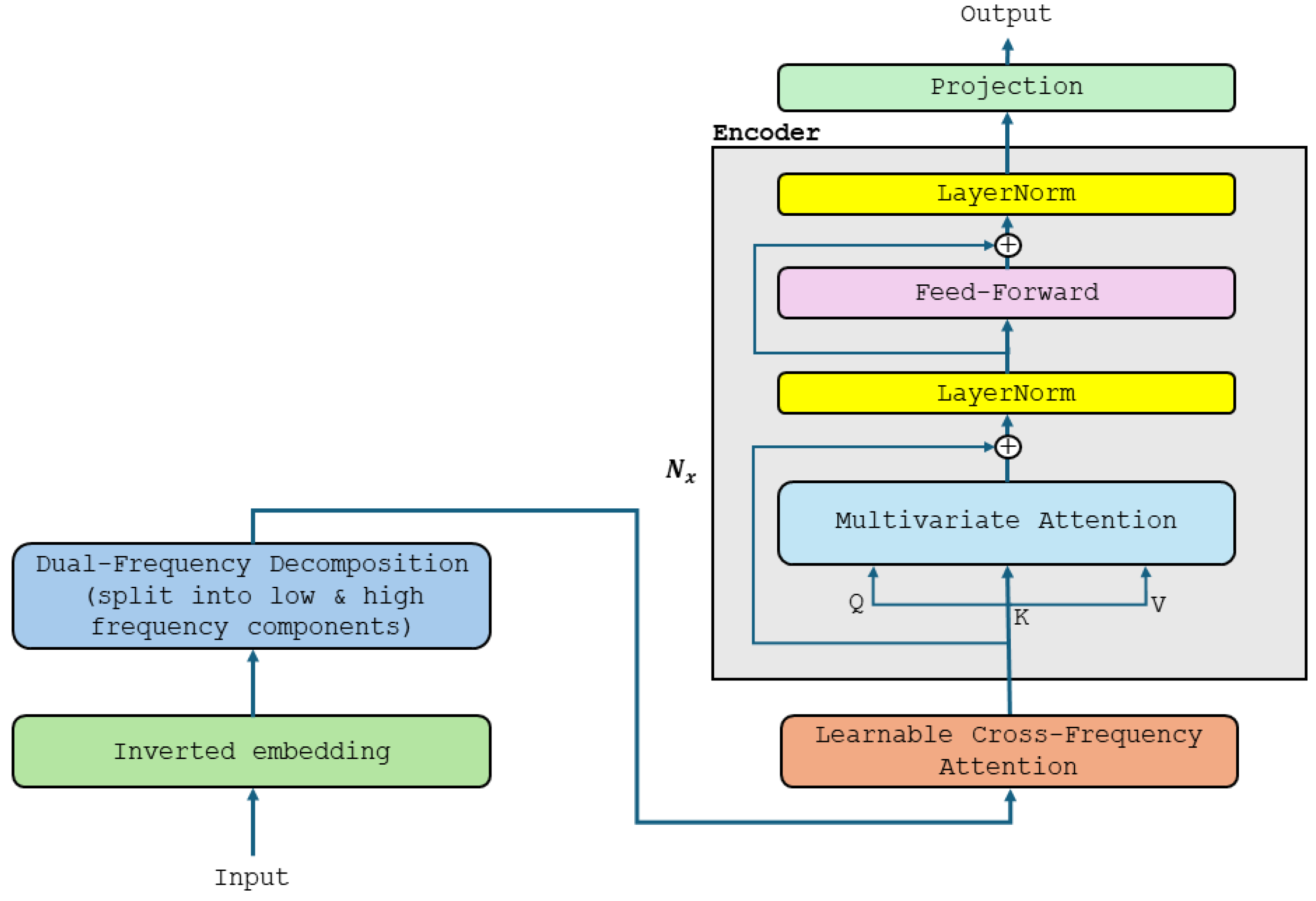
This study critically evaluates the trade-offs between complexity and performance by examining two variants of the base inverted Transformer (iTransformer) model. The first, Memory iTransformer (MiTransformer), augments the iTransformer by incorporating a memory-augmented module (MAM), introduced in [3] to capture long-range dependencies. The second, Dual-Frequency iTransformer (DFiTransformer), introduces a dual-frequency decomposition (DFD) module that splits the embedded sequence into low- and high-frequency components, which are subsequently fused via a Learnable Cross-Frequency Attention (LCFA) mechanism to enhance frequency-aware learning.
Despite their theoretical promise, both MiTransformer and DFiTransformer exhibit degraded forecasting accuracy compared to the simpler iTransformer across a suite of benchmarks. This result supports emerging findings in the literature that in some contexts, simpler models outperform their more complex counterparts [4,5], highlighting the importance of parsimony and interpretability, especially in real-world deployment contexts.
To support our analysis, we include architecture diagrams (see Figure 1 and Figure 2) that illustrate the structural differences between MiTransformer and DFiTransformer. These visualizations help clarify the design intentions behind each model and provide context for interpreting their relative performance.

2. Related Work

Transformer-based models have quickly become popular in TSF because of their capacity to capture long-range dependencies and adaptable attention mechanisms. Early adaptations such as the Informer [6] and Autoformer [7] introduced efficiency improvements via sparse attention and series decomposition. These models paved the way for further innovations aimed at enhancing the temporal modelling capabilities of transformers.
Building on this foundation, the iTransformer [2] introduced an inverted structure that processes input along the variable dimension, demonstrating competitive performance with a remarkably simple architecture. This idea of “less is more” has recently gained renewed attention in the field, particularly with models like PatchTST [8], which emphasized architectural minimalism and achieved strong empirical results.
In contrast, more complex designs have sought to boost performance by integrating advanced components. FiLM [9] explored frequency-based modelling, while FEDformer [10] introduced frequency-enhanced decompositions. Some models employ the inclusion of external memory systems to improve their capability to remember remote temporal patterns [11]. Inspired by memory networks [12], MAMs aim to address memory decay over long horizons.
Similarly, the MiTransformer introduced in this study incorporates a MAM (introduced in [3]) into iTransformer, drawing inspiration from the effectiveness of memory-augmented transformers in both NLP and vision applications [13,14]. It improves the performance of MAMs, which focus on overcoming the limitations of traditional attention in efficiently modelling long-term dependencies. Although MAMs have been proposed to address long-range dependencies in sequential data, their benefits must be weighed against the increased complexity of inference and resource demands [15].
The DFiTransformer introduced here represents another complexity-oriented extension. It incorporates dual-frequency decomposition to separate embedded signals into low- and high-frequency components and fuses them using an LCFA mechanism. This design shares conceptual ties with frequency-aware models like FEDformer and FiLM but adopts a learnable fusion strategy rather than fixed or heuristic mechanisms.
Despite these architectural enhancements, our results indicate that such complexity may not yield better forecasting outcomes. Transformer-based models provide effective scalability and performance in time series tasks; however, enhancing architectural complexity does not automatically result in improved accuracy, particularly in the context of distribution shifts or extended prediction horizons [4], as evidenced in our study. The simpler iTransformer consistently outperforms both MiTransformer and DFiTransformer across various datasets and forecasting horizons. This observation echoes a growing body of research [2,4] that advocates for simplicity in time series model design, citing benefits in generalization, interpretability, and practical deployment.

3. Methodology

The usefulness of simplicity versus complexity in transformer-based models for multivariate TSF is examined in this work. We assess three model variations—iTransformer, MiTransformer, and DFiTransformer—which have different architectural complexities but are all based on the inverted transformer architecture. The baseline model, iTransformer, is distinguished by its inverted transformer architecture, which handles time series inputs without the need for a decoder. By eschewing common autoregressive elements, it prioritizes simplicity and uses an effective encoder-only framework to enable direct sequence-to-sequence forecasting.
MiTransformer (Figure 1) extends the iTransformer architecture by integrating a memory-augmented module (MAM) into each encoder layer. The MAM introduces a fixed-size, learnable memory bank that explicitly stores past representations and dynamically retrieves relevant historical patterns using cross-attention mechanisms. This design enables the model to offload long-term contextual information from the self-attention layers, mitigating memory decay over long input sequences.
Specifically, the MAM interacts with the encoder’s hidden states by projecting them into a query space and attending over memory slots to retrieve useful summaries of prior temporal dynamics. The memory bank is updated iteratively via gating mechanisms that balance the retention of old memory with the integration of new inputs. By enhancing long-range dependency modelling, MiTransformer is better suited for datasets with extended seasonalities or global trends. However, this added capability comes at the cost of increased architectural complexity and computational overhead.
DFiTransformer introduces DFD and an LCFA mechanism to enhance the modelling of multi-scale temporal dependencies. Instead of integrating a memory component, DFiTransformer decomposes the encoded sequence into low-frequency (trend-like) and high-frequency (residual-like) components using average pooling and residual subtraction. Each frequency component is then processed independently, and their outputs are fused through a learnable cross-attention mechanism that captures inter-frequency interactions. The resulting representation is passed into the standard Transformer encoder stack without altering its internal attention operations.
By explicitly modelling frequency bands, DFiTransformer aims to handle multi-scale temporal dynamics more effectively than conventional architectures. However, it introduces additional components and attention layers, increasing the model’s depth and computational burden while lacking explicit memory mechanisms to retain past information.
Every model is assessed under the same conditions through various public datasets utilizing standard metrics (MSE and MAE). The aim of this controlled comparison is to investigate if architectural advancements, like memory enhancement or frequency alteration, reliably surpass the basic iTransformer baseline.
The characteristics of the aforementioned Transformer-based models are summarized below:
  • iTransformer: Prioritizes simplicity and speed. Strong baseline.
  • MiTransformer: Adds memory augmentation to capture long-term temporal dependencies, performing better on datasets with recurrent patterns.
  • DFiTransformer: Focuses on frequency-aware modelling and complex interactions, useful for multi-scale signals, but can be computationally expensive and prone to overfitting.
Finally, the iTransformer is the simplest of the three while DFiTransformer is the most complex, as shown in the Appendix A.

4. Experimental Setup

We evaluate the performance of three Transformer-based models—iTransformer, MiTransformer, and DFiTransformer—on widely used multivariate time series forecasting benchmarks under the multi-step forecasting framework. In this setup, each model predicts the next L future time steps given a fixed-length historical window.
We consider forecasting lengths of 96, 192, 336, and 720 time steps in order to evaluate predictive accuracy over both short- and long-term horizons. Two common metrics are used for evaluation: Mean Absolute Error (MAE) and Mean Squared Error (MSE). To allow for fair comparison across datasets of different scales, both metrics are reported in their normalized form. Better forecasting performance is indicated by lower values in these metrics.
For experimental consistency and to isolate the effect of model architecture, we adopt a uniform input sequence length of 96 time steps across all models and forecast horizons. This fixed input length is commonly used in the literature and provides a controlled basis for comparing model behaviour at varying prediction horizons.
Furthermore, a shared training configuration is applied across all models using PyTorch version 1.13.1 and trained on an NVIDIA A8000 80 G GPU (Santa Clara, CA, USA). The Adam optimiser is used to train the model with a batch size of 32, a dropout rate of p = 0.1, and an initial learning rate of 0.0001 that decreases by two times each epoch. To avoid overfitting, we implement early stopping once the model has gone ten consecutive epochs without learning.
These hyperparameters were selected based on preliminary runs and align with standard TSF practices. While we acknowledge that fine-tuning hyperparameters for each architecture may offer marginal performance gains, doing so risks biasing the evaluation in favour of certain models. Therefore, fixed hyperparameters are employed intentionally to ensure a fair, controlled, and reproducible comparison, emphasizing architectural simplicity versus complexity rather than training nuances.
By harmonizing both evaluation protocol and implementation settings, this setup provides a rigorous, reproducible framework for analyzing performance trade-offs and a principled examination of how architectural changes (e.g., frequency encoding, dynamic filtering) affect generalization and robustness across diverse datasets.

4.1. Datasets

We evaluate the models using five widely used multivariate time series datasets:
  • Weather: Meteorological data from the US, including variables like temperature, humidity, and wind speed.
  • Electricity Consumption Load (ECL): Hourly electricity consumption data of 321 clients.
  • Exchange: Daily exchange rates of eight different countries.
  • ETTm1 and ETTm2: Electric Transformer Temperature datasets with different temporal resolutions (15 min and 1 h intervals).
Each dataset is split into training, validation, and testing sets using a standard 7:2:1 ratio.

4.2. Models Compared

  • iTransformer: The baseline inverted transformer architecture.
  • MiTransformer: Enhances iTransformer with a memory-augmented module.
  • DFiTransformer: Adds DFD and LCFA to iTransformer.
All models are implemented in PyTorch and trained under consistent hyperparameter settings to ensure comparability.

5. Results and Analysis

We evaluated iTransformer, MiTransformer, and DFiTransformer across five widely used time series forecasting benchmarks, using MSE and MAE as evaluation metrics. Forecasting horizons of 96, 192, 336, and 720 steps were considered to test performance at increasing levels of difficulty. Table 1 presents the results of forecasting.
Across all datasets and forecasting horizons, the iTransformer consistently achieves the lowest average errors. MiTransformer, which adds a memory-augmented mechanism to the iTransformer, shows a marginal performance drop, particularly on long-term horizons. However, the DFiTransformer, despite being the most complex—introducing dual-frequency decomposition and cross-frequency attention—underperforms relative to both simpler models, especially on challenging datasets like Exchange and ECL.
For example, on the Exchange dataset, iTransformer achieves an average MSE of 0.360 compared to 0.366 for MiTransformer and 0.438 for DFiTransformer. A similar trend holds for ECL, where the average MSEs are 0.178, 0.193, and 0.217, respectively. Notably, performance gaps widen with increasing prediction lengths, suggesting that added architectural complexity may hinder long-term generalization.
These findings reinforce our central claim; architectural simplicity not only facilitates interpretability and efficiency but also tends to generalize better in practical forecasting scenarios. Even modest enhancements, such as the external memory module in MiTransformer, can introduce unnecessary overhead without clear performance benefits. The performance degradation observed in DFiTransformer further illustrates that increased model complexity does not guarantee improved outcomes, especially in the domain of time series forecasting.

6. Discussion: Simplicity vs. Complexity in Forecasting Models

Our comparative evaluation of three transformer-based models—iTransformer, MiTransformer, and DFiTransformer—reveals a consistent and important trend; simpler architectures can outperform more complex designs in time series forecasting. Studies have shown that simpler models, in some cases, outperform more complex ones due to their generalization ability and reduced computational demands [9,13].
The iTransformer, employing a minimal inverted attention mechanism without auxiliary modules, delivers robust and consistent results across diverse datasets. In contrast, MiTransformer, which introduces a memory-augmented component, and DFiTransformer, which integrates frequency decomposition and cross-frequency attention, exhibit diminished performance despite increased architectural sophistication.
These findings challenge the prevailing assumption that architectural complexity necessarily leads to better forecasting accuracy. In fact, the performance degradation observed in MiTransformer and DFiTransformer suggests that additional modules may introduce noise or overfitting—particularly problematic in real-world time series that are often noisy and non-stationary. This means that our findings agree with [14,16], who show that strong inductive biases or lightweight architectural designs can lead to superior generalization on long-range dependencies. Also, our findings echo those of [5], where a simple linear model outperformed state-of-the-art Transformer variants on long-term time-series forecasting.
The implications are twofold. First, for practical deployment, models like iTransformer offer favourable trade-offs between accuracy, computational cost, and interpretability. Second, from a research perspective, our results call for a more nuanced understanding of architectural design; simplification, not complication, may be key to generalizable and scalable forecasting solutions.
Our experimental results across six benchmark datasets reveal a consistent trend; increasing architectural complexity does not guarantee performance improvement in time series forecasting. The original iTransformer often outperforms both MiTransformer, which adds a memory augmentation module, and DFiTransformer, which combines memory with dual-frequency attention mechanisms. Among the three, DFiTransformer—the most complex—achieves the weakest performance on average. This hierarchy of results strongly supports the insight that simpler architectures not only generalize better but also offer practical advantages in terms of training efficiency and model interpretability [2,8]. Therefore, our findings reinforce the principle that more is not always better—especially when it comes to deep learning for sequential data. These findings suggest that future model development should prioritize principled minimalism, seeking targeted, lightweight improvements rather than wholesale architectural expansion.

7. Conclusions

This paper assessed two improved versions of the iTransformer—MiTransformer and DFiTransformer—each meant to enhance the base model via memory augmentation and frequency-aware mechanisms, respectively. Though they added complexity, both models fell short of the original iTransformer. These findings support the growing body of evidence indicating that in time series forecasting, architectural simplicity often produces better generalization and robustness. Our results support the case that, particularly for long-term forecasting, more complex designs do not ensure better performance—highlighting the idea that “the simpler, the better” remains a useful design philosophy.

Author Contributions

P.S.Y.: conceptualisation, methodology, software, formal analysis, writing—original draft; X.M.: supervision, conceptualisation; D.S.: conceptualisation and review; C.Y.: software, code validation; V.A.O. and A.I.: writing—review and editing. All authors have read and agreed to the published version of the manuscript.

Funding

Not applicable. This research did not receive any specific grant from funding agencies in the public, commercial, or not-for-profit sectors.

Institutional Review Board Statement

Not applicable.

Informed Consent Statement

Not applicable.

Data Availability Statement

Primary datasets: iTransformer official Google Drive. available online: https://drive.google.com/file/d/1l51QsKvQPcqILT3DwfjCgx8Dsg2rpjot/view (accessed 12 January 2025); Informer official Google Drive available online: https://drive.google.com/drive/folders/1ohGYWWohJlOlb2gsGTeEq3Wii2egnEPR(accessed 22 September 2024); ETT Datasets. available online::https://github.com/zhouhaoyi/. ETDatasetPre-processing code: A public GitHub repository. available online: https://github.com/ypolycarp/SimplicityComplexity. (accessed 12 January 2025) will be activated upon acceptance.

Acknowledgments

We thank and acknowledge the Computer Networks Lab, School of Electronic and Information Engineering, Liaoning Technical University for providing computational resources for our experiments.

Conflicts of Interest

The authors declare no competing interests.

Appendix A

To perform actual calculations of parameter count and simplicity between iTransformer, MiTransformer, and DFiTransformer, we assume the following common baseline settings for fairness:
  • Input sequence length: 96.
  • Correct full multi-head attention (MHA) parameter count: 4 × d_model2.
  • Feedforward layer: 2 × d_model × d_ff.
  • Consistent dimensions:
    d_model = 512;
    d_ff = 2048;
    #layers = 2;
    #heads = 8 (used in attention logic, but does not affect parameter count).
Model Parameter Breakdown (per layer)
Each Transformer encoder layer:
  • MHA (Q + K + V + Output): 4 × 5122 = 1,048,576.
  • Feedforward: 2 × 512 × 2048 = 2,097,152.
  • Total per layer = 1,048,576 + 2,097,152 = 3,145,728.
For 2 layers → 2 × 3,145,728 = 6,291,456
Model-by-Model Calculation
1. iTransformer
  • Input embedding: 512 × 1 = 512.
  • Transformer encoder: 6,291,456.
  • Output layer: 512 × 1 = 512.
  • Total → 6,291,456 + 512 + 512 = 6,292,480.
Final: ~6.29 M parameters
2. MiTransformer (with MAM)
  • iTransformer base: 6,292,480
  • Added components:
    Memory slots: M = 64, each slot = 512
    → 64 × 512 = 32,768.
    Memory attention: same projection scheme as MHA
    → 4 × 5122 = 1,048,576.
  • Total → 6,292,480 + 32,768 + 1,048,576 = 7,373,824
Final: ~7.37 M parameters
3. DFiTransformer
  • iTransformer base: 6,292,480.
  • Added components:
    Dual-frequency token projections (2 branches): 2 × 512 × 512 = 524,288.
    Cross-frequency attention: 4 × 5122 = 1,048,576.
    Fusion layer (linear): 512 × 512 = 262,144.
  • Total → 6,292,480 + 524,288 + 1,048,576 + 262,144 = 8,127,488.
Final: ~8.13 M parameters
Final Comparison Table
ModelParameter CountExtra ModulesComplexity Level
iTransformer~6.29 M(1)
MiTransformer~7.37 MMemory slots + attention(2)
DFiTransformer~8.13 MDFD + LCFA (3)
Insights:
  • iTransformer is the most parameter-efficient and easiest to interpret;
  • MiTransformer increases parameters moderately with significant benefit on periodic or long-range data;
  • DFiTransformer adds even more complexity, useful in frequency-rich datasets, but has diminishing returns on simple tasks.

References

  1. Vaswani, A.; Shazeer, N.; Parmar, N.; Uszkoreit, J.; Jones, L.; Gomez, A.N.; Kaiser, Ł.; Polosukhin, I. Attention is all you need. In Proceedings of the 31st Conference on Neural Information Processing Systems (NIPS 2017), Long Beach, CA, USA, 4–9 December 2017. [Google Scholar]
  2. Liu, Y.; Hu, T.; Zhang, H.; Wu, H.; Wang, S.; Ma, L.; Long, M. itransformer: Inverted transformers are effective for time series forecasting. In Proceedings of the ICLR 2024, Vienna, Austria, 7–11 May 2024. [Google Scholar]
  3. Yakoi, P.S.; Meng, X.; Yu, C.; Odeh, V.A.; Zhang, Y.; Zhao, Z.; Suleman, D.; Yang, Y. LTSMiTransformer: Learnable Temporal Sparsity and Memory for Efficient Long-Term Time Series Forecasting. In Proceedings of the 2025 6th International Conference on Computing, Networks and Internet of Things (CNIOT), Shanghai, China, 23–25 May 2025; pp. 1–7. [Google Scholar]
  4. Zeng, A.; Chen, M.; Zhang, L.; Xu, Q. Are transformers effective for time series forecasting? Proc. AAAI Conf. Artif. Intell. 2023, 37, 11121–11128. [Google Scholar] [CrossRef]
  5. Chen, H.; Luong, V.; Mukherjee, L.; Singh, V. SimpleTM: A Simple Baseline for Multivariate Time Series Forecasting. In Proceedings of the Thirteenth International Conference on Learning Representations, Singapore, 24–28 April 2025. [Google Scholar]
  6. Zhou, H.; Zhang, S.; Peng, J.; Zhang, S.; Li, J.; Xiong, H.; Zhang, W. Informer: Beyond efficient transformer for long sequence time-series forecasting. Proc. AAAI Conf. Artif. Intell. 2021, 35, 11106–11115. [Google Scholar] [CrossRef]
  7. Wu, H.; Xu, J.; Wang, J.; Long, M. Autoformer: Decomposition transformers with auto-correlation for long-term series forecasting. In Proceedings of the 35th Conference on Neural Information Processing Systems (NeurIPS 2021), Online, 6–14 December 2021. [Google Scholar]
  8. Nie, Y.; Nguyen, N.H.; Sinthong, P.; Kalagnanam, J. A time series is worth 64 words: Long-term forecasting with transformers. arXiv 2022, arXiv:2211.14730. [Google Scholar]
  9. Lim, B.; Zohren, S. Time-series forecasting with deep learning: A survey. Philos. Trans. R. Soc. A 2021, 379, 20200209. [Google Scholar] [CrossRef] [PubMed]
  10. Zhou, T.; Ma, Z.; Wen, Q.; Wang, X.; Sun, L.; Jin, R. Fedformer: Frequency enhanced decomposed transformer for long-term series forecasting. In Proceedings of the International Conference on Machine Learning, Baltimore, MD, USA, 17–23 July 2022. [Google Scholar]
  11. Rae, J.; Hunt, J.J.; Danihelka, I.; Harley, T.; Senior, A.W.; Wayne, G.; Graves, A.; Lillicrap, T. Scaling memory-augmented neural networks with sparse reads and writes. Adv. Neural Inf. Process. Syst. 2016, 29, 3628–3636. [Google Scholar]
  12. Sukhbaatar, S.; Weston, J.; Fergus, R. End-to-end memory networks. Adv. Neural Inf. Process. Syst. 2015, 28, 2440–2448. [Google Scholar]
  13. Elsayed, S.; Thyssens, D.; Rashed, A.J.H.S.; Schmidt-Thieme, L. Do we really need deep learning models for time series forecasting? arXiv 2021, arXiv:2101.02118. [Google Scholar] [CrossRef]
  14. Wu, H.; Hu, T.; Liu, Y.; Zhou, H.; Wang, J.; Long, M. Timesnet: Temporal 2d-variation modeling for general time series analysis. arXiv 2022, arXiv:2210.02186. [Google Scholar]
  15. Kaiser, Ł.; Nachum, O.; Roy, A.; Bengio, S. Learning to remember rare events. arXiv 2017, arXiv:1703.03129. [Google Scholar] [CrossRef]
  16. Gu, A.; Dao, T. Mamba: Linear-time sequence modeling with selective state spaces. arXiv 2023, arXiv:2312.00752. [Google Scholar] [CrossRef]
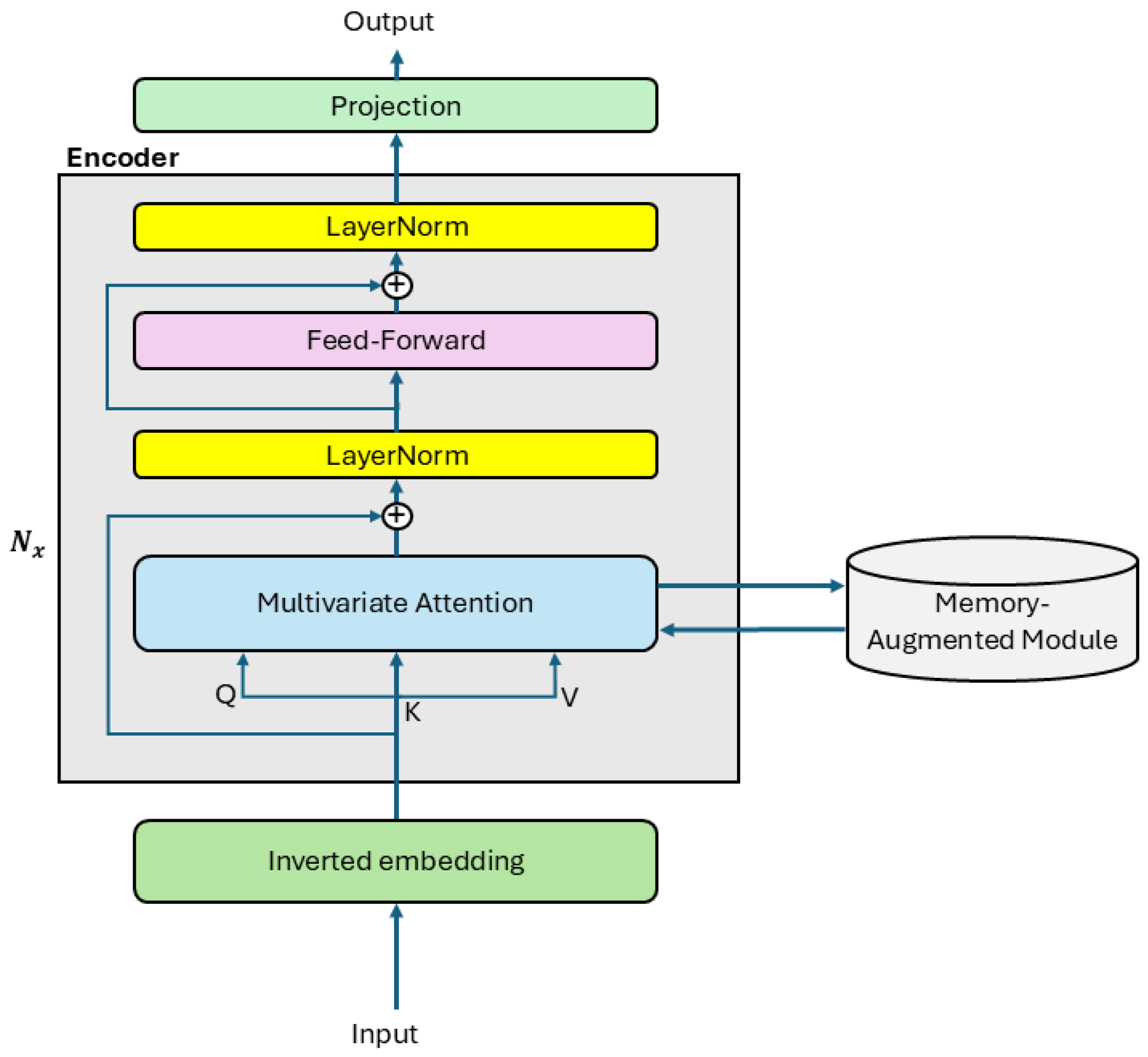
Figure 1. MiTransformer architecture.
Csmf 11 00027 g001
Figure 2. DFiTransformer architecture.
Csmf 11 00027 g002
Table 1. Forecasting results.
ModelsiTransformerMiTransformerDFiTransformer
MetricMSEMAEMSEMAEMSEMAE
Weather960.1740.2140.1790.2180.1870.232
1920.2210.2540.2240.2570.2420.275
3360.2780.2960.2850.3010.2990.313
7200.3580.3470.3590.3500.3730.364
Macro Avg0.2580.2780.2620.2820.2750.296
ECL960.1480.2400.1660.2560.1910.297
1920.1620.2530.1770.2670.2070.310
3360.1780.2690.1950.2850.2220.323
7200.2250.3170.2340.3180.2490.343
Macro Avg0.1780.2700.1930.2820.2170.318
Exchange960.0860.2060.0870.2070.1190.245
1920.1770.2990.1760.2990.2520.358
3360.3310.4170.3460.4260.4300.475
7200.8470.6910.8540.7000.9490.738
Macro Avg0.3600.4030.3660.4080.4380.454
ETTm1960.3340.3680.3540.3820.3680.392
1920.3770.3910.3830.3940.4110.415
3360.4260.4200.4440.4300.4440.437
7200.4910.4590.5170.4700.5600.493
Macro Avg0.4070.4100.4250.4190.4460.434
ETTm296.0000.1800.2640.1820.2630.1960.275
192.0000.2500.3090.2500.3060.2560.313
336.0000.3110.3480.3180.3510.3320.358
720.0000.4120.4070.4140.4050.4140.404
Macro Avg0.2880.3320.2910.3310.3000.338
1st24242201
2nd11232330
Note: “Macro Avg” is the unweighted average across the four horizons. Red results are the best, and the blue results are the 2nd best.
Disclaimer/Publisher’s Note: The statements, opinions and data contained in all publications are solely those of the individual author(s) and contributor(s) and not of MDPI and/or the editor(s). MDPI and/or the editor(s) disclaim responsibility for any injury to people or property resulting from any ideas, methods, instructions or products referred to in the content.