Proceeding Paper

Enhancing Public Health Insights and Interpretation Through AI-Driven Time-Series Analysis: Hierarchical Clustering, Hamming Distance, and Binary Tree Visualization of Infectious Disease Trends †

by
Ayauzhan Arystambekova
and
Eugene Pinsky
*
*
Author to whom correspondence should be addressed.
Presented at the 11th International Conference on Time Series and Forecasting, Canaria, Spain, 16–18 July 2025.
All authors contributed equally to this work.
Comput. Sci. Math. Forum 2025, 11(1), 23; https://doi.org/10.3390/cmsf2025011023
Published: 11 August 2025

Abstract

This paper applies hierarchical clustering and Hamming Distance to analyze the temporal trends of infectious diseases across different regions of Uzbekistan. By leveraging hierarchical clustering, we effectively group regions based on disease similarity without requiring predefined cluster numbers. Hamming Distance further quantifies disease trajectory similarities, helping assess epidemiological patterns over time. Binary tree visualizations enhance the interpretability of clustering results, offering a novel method for identifying regional trends. The dataset includes yearly incidence rates of seven infectious diseases from 2012 to 2019, along with population, healthcare infrastructure, and geographic attributes for each region. This approach provides an interpretable framework for public health analysis and decision-making.

1. Introduction

Effective monitoring of infectious diseases is crucial for public health forecasting and intervention. Traditional methods often face challenges with high-dimensional, noisy, and irregular data, complicating the detection of spatio-temporal trends. Identifying regional similarities in disease outbreaks can help policymakers allocate resources efficiently and track disease dynamics.
Recently, machine learning has proven effective at identifying patterns in disease spread. Conventional clustering methods like K-Means or DBSCAN, however, rely on predefined parameters (e.g., number of clusters or distance thresholds), limiting their flexibility when analyzing diverse and evolving disease outbreaks.
To overcome these challenges, this study uses Hierarchical Clustering, which does not require predefined parameters and is flexible enough to group regions based on natural similarities in disease trends. This ability is especially valuable in epidemiology, where disease clustering can vary over time. Hamming Distance is employed to quantify year-over-year differences in disease prevalence, particularly for categorical or binary data, enabling a precise assessment of disease dynamics. By integrating these two methods, we create a framework for analyzing both spatial and temporal trends in infectious disease patterns.

1.1. Contributions of This Study

The primary contributions of this study are as follows:
  • Hierarchical Clustering for Disease Classification
    Automatically determines regional clusters of disease prevalence without requiring a predefined number of clusters.
    Provides a dendrogram-based representation to capture hierarchical relationships among regions.
  • Hamming Distance for Time-Series Similarity
    Quantifies year-over-year variations in disease trajectories, allowing detection of significant shifts in prevalence.
    Identifies epidemiologically similar regions based on shared trends over time.
  • Binary Tree Visualization for Improved Interpretation
    Introduces binary trees to represent disease clustering in a more interpretable structure.
    Helps health professionals track regional transitions in disease prevalence and detect outlier patterns.
  • Evaluation of Compactness and Variability
    Incorporates compactness scores to measure intra-cluster consistency and inter-cluster distinctiveness.
    Uses silhouette score analysis to validate cluster separations.

1.2. Case Study: Infectious Diseases in Uzbekistan

Uzbekistan, a Central Asian country with diverse geographic and economic regions, provides an ideal case study for evaluating disease clustering methods. The dataset analyzed includes seven infectious diseases recorded from 2010 to 2019 across 13 administrative regions.
By applying hierarchical clustering and Hamming Distance, we uncover key regional differences in disease patterns, helping policymakers understand which regions share similar epidemiological profiles and which require targeted interventions.

1.3. Organization of the Paper

This paper is structured as follows:
  • Section 2 provides a detailed description of the dataset, highlighting the key attributes analyzed.
  • Section 3 presents the methodology, outlining the clustering techniques, Hamming Distance calculations, and visualization methods.
  • Section 4 describes the case study findings, illustrating the application of the proposed methods in analyzing disease trends across regions.
  • Section 5 discusses the implications of the results and suggests future improvements.
  • Section 6 concludes the study, summarizing the key findings and future research directions.
By combining unsupervised learning techniques with interpretability-focused visualizations, this study aims to enhance the precision and transparency of infectious disease analysis, offering a reproducible framework for public health research and intervention planning.

2. Dataset Description

This study uses publicly available epidemiological data from Uzbekistan’s e-Government portal https://data.egov.uz/eng (accessed on 30 June 2025). The dataset includes annual infectious disease incidence rates across 13 regions from 2010 to 2019, structured as a time series to facilitate clustering techniques such as Hamming Distance for detecting temporal and regional disease patterns.These regions are shown in Figure 1.

2.1. Data Attributes

The dataset includes the following key attributes:
  • Region ID and Name: Unique identifier and administrative name for each region.
  • Disease Type: The dataset includes seven infectious diseases—Brucellosis, Dysentery, Measles, Tuberculosis, Scarlet Fever, Typhoid Fever, and Meningococcal Infections.
  • Yearly Incidence Rate: The number of reported cases per 100,000 people for each disease.
  • Geographical Coordinates: Latitude and longitude values representing the central location of each region.
These attributes allow us to track the spatial and temporal evolution of infectious diseases and explore correlations between disease prevalence, geographic distribution, and healthcare resources.

2.2. Data Preprocessing

The preprocessing steps were as follows:
  • Data Cleaning: Duplicate and inconsistent entries were removed.
  • Handling Missing Data: Missing incidence rates were imputed using the mean prevalence for the respective region and disease type.
  • Standardization: Ensured consistency in temporal analysis across regions and disease types.
These preprocessing steps prepare the dataset for the application of temporal clustering techniques like Hamming Distance, which is particularly useful for capturing year-over-year variations in disease incidence.

Time-Series Structuring

For analysis, each disease’s incidence rate per region was structured as a time-series dataset:
  • Each row represents a unique region-disease combination with time-series values spanning 2010 to 2019.
  • Disease trends are analyzed across multiple time scales (e.g., yearly aggregates and multi-year comparisons).

2.3. Regional Classification and Economic Zones

To enhance the interpretability of disease clustering, the dataset includes a classification of regions into economic zones based on population density, dominant economic activity, and healthcare infrastructure. Table 1 provides an overview of these classifications.
The classification into Industrialized, Agricultural, Emerging, and Less Developed zones is based on:
  • Industrialized Zones: Highly urbanized regions with developed healthcare infrastructure (e.g., Tashkent City, Navoi).
  • Agricultural Zones: Predominantly rural regions with agriculture as the primary economic activity (e.g., Andijan, Namangan).
  • Emerging Zones: Regions undergoing rapid development but still facing healthcare accessibility challenges (e.g., Samarkand, Jizzakh).
  • Less Developed Zones: Remote or historically underdeveloped regions with limited healthcare resources (e.g., Karakalpakstan, Khorezm).

2.4. Geographical Indicators

Geographical coordinates were used to compare similarities and differences among regions located next to each other or further apart. The spatial proximity of regions plays a crucial role in infectious disease spread, making the integration of geographic indicators essential for clustering analysis.
The inclusion of regional classification and geographic coordinates allows for an advanced hierarchical clustering approach, ensuring that the disease trends are interpreted not just by numerical similarity but also by spatial context.
The code and data used in this study are available at https://github.com/ayau6591/AI_tools_UZ (accessed on 30 June 2025).

3. Literature Review

The study of infectious disease patterns has advanced significantly with developments in data science, applying methods such as time-series analysis and spatial clustering to derive actionable public health insights [1,2]. Although traditional approaches remain valuable, they often struggle to capture geographic and temporal patterns. Machine learning techniques, particularly clustering algorithms [3,4,5], have addressed some of these limitations by identifying clusters based on disease prevalence, enabling more targeted health interventions. However, effective integration of spatial and temporal data remains a challenge.
Hierarchical clustering has been extensively studied in both theory and practice. Foundational texts such as Data Mining: Concepts and Techniques [6] and Introduction to Data Mining [7] provide comprehensive overviews of clustering methodologies, including hierarchical methods. Jain’s survey, “Data Clustering: 50 Years Beyond K-Means” [5], offers a broad analysis, situating hierarchical techniques within modern applications.
Cluster analysis has diverse applications in public health. For example, Porter [8] discusses its role in regional economic development, while Lai [9] examines spatial clustering in disease transmission. Anselin’s work on spatial clustering and Geographic Information Systems (GIS) [10] provides a foundation for understanding geographic patterns in health research. More recently, Sadeghi et al. [11] applied hierarchical clustering to evaluate COVID-19 preperadness and response across 180 countries, demonstrating its value for global pandemic monitoring and cross-country comparison.
Clustering methods are widely used in infectious disease research. For example, Pattnaik et al. [12] use Hamming Distance to group disease patterns and to study how diseases spread in urban and rural areas. Brauer’s work [13] blends mathematical modeling with data analysis, offering robust methods to understand disease dynamics. Binary tree visualizations, essential for interpreting hierarchical clustering results, are detailed in key resources such as The Algorithm Design Manual by Skiena [14] and Introduction to Algorithms by Cormen et al. [15].
The temporal aspects of disease patterns are equally important. Foundational contributions by George E.P. Box and Gwilym Jenkins [16] on the Box–Jenkins method provide essential tools for analyzing time-series data. Rob J. Hyndman and George Athanasopoulos [17] extend these ideas with modern techniques in Forecasting: Principles and Practice, making them particularly relevant for temporal disease clustering. Real-time clustering methods are explored in the work of Charu C. Aggarwal [18], who addresses dynamic data streams and their applications in public health. Similarly, Hulten [19] contributes to understanding the changing data streams that evolve over time, which are crucial for real-time disease tracking and response.
Building on this foundation, our study integrates hierarchical clustering with the Hamming Distance to analyze infectious disease patterns. By visualizing hierarchical clustering results as binary trees, we enhance the interpretability of temporal and regional patterns, offering a clearer understanding of health disparities and supporting data-driven public health strategies [8,20,21,22]. We assess the reliability of clustering results across years by evaluating compactness, silhouette scores, and dendrogram cut-offs, following the general stability considerations discussed by Nogueira and Brown [23].

4. Methodology

The methodology demonstrates the framework’s options for analyzing disease patterns across two hypothetical regions, Region 1 and Region 2. Each region is represented by a set of diseases, with Region 1 defined by a set of variables X and Region 2 by a set of variables T. We employ a variety of techniques to analyze disease prevalence patterns and assess the robustness of clustering results.

4.1. Notation and Symbol Definitions

To ensure clarity in the mathematical formulation, we define the notation used throughout this study. This is shown in Table 2.
These symbols will be used in equations throughout the methodology section.

4.2. Hierarchical Clustering

Hierarchical clustering is an unsupervised learning technique used to group similar objects based on their attributes without requiring a predefined number of clusters. Unlike methods such as K-Means, which require an initial cluster count, hierarchical clustering identifies natural groupings by iteratively merging smaller clusters.
In this study, we apply hierarchical clustering to disease prevalence data across different regions in Uzbekistan. To measure cluster similarity, we use Ward’s method, which minimizes the total within-cluster variance when merging clusters.
The change in error sum of squares ( Δ E S S ) when merging two clusters C 1 and C 2 is given by
Δ E S S = i C 1 C 2 x i μ ( C 1 C 2 ) 2 i C 1 x i μ ( C 1 ) 2 + i C 2 x i μ ( C 2 ) 2
where
  • C 1 and C 2 are the clusters being merged;
  • x i represents a data point in a cluster;
  • μ ( C 1 ) , μ ( C 2 ) , and μ ( C 1 C 2 ) are the centroids of clusters C 1 , C 2 , and their merged cluster, respectively.
The output of hierarchical clustering is a dendrogram, which visually represents how clusters are formed at different levels of similarity.

4.3. Cluster Selection for Region 1 and Region 2

4.3.1. Dendrogram Analysis

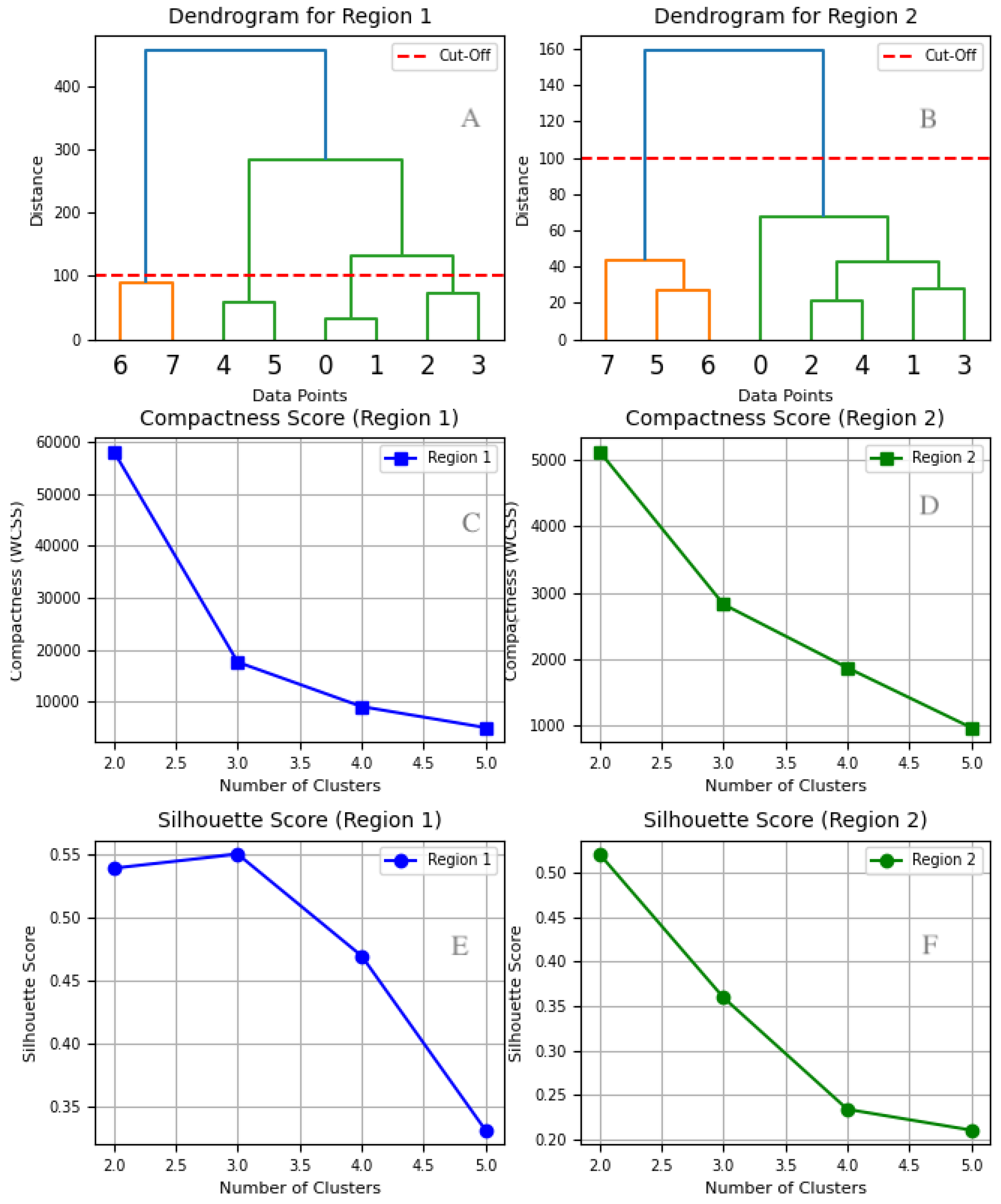
The hierarchical clustering dendrograms as well as compactness and silhouette scores for both regions are presented in Figure 2 (top row). A cutoff threshold (red dashed line) was selected to balance cluster separation and compactness.
For Region 1, the dendrogram suggests a natural grouping of diseases into three clusters. For Region 2, a two-cluster structure is more appropriate due to lower variability in disease patterns. However, since clustering compactness and silhouette scores were evaluated for 2 to 5 clusters, we also examine whether additional clusters improve the model.

4.3.2. Compactness Score (WCSS)

The Within-Cluster Sum of Squares (WCSS) measures how tightly data points are grouped within a cluster. Lower WCSS values indicate more compact clusters.
Figure 2 (middle row) shows the following:
  • For Region 1, the WCSS score drops significantly from two to three clusters, then continues declining at a slower rate beyond three. While additional clusters slightly improve compactness, the diminishing returns suggest that further separation offers limited benefit.
  • For Region 2, the most notable drop occurs between one and two clusters, followed by a gradual decline. This indicates that two clusters provide the best balance between compactness and model simplicity.

4.3.3. Silhouette Score Analysis

The silhouette score evaluates clustering quality by measuring the cohesion within clusters and separation between clusters. A higher silhouette score indicates well-defined clusters.
From Figure 2 (bottom row), the following are observed:
  • For Region 1, the highest silhouette score occurs at three clusters. While four and five clusters result in a steady decline in silhouette scores, three clusters maintain the best cluster cohesion and separation.
  • For Region 2, the highest silhouette score is observed at two clusters, confirming that additional clusters reduce the clustering quality.

4.3.4. Final Cluster Selection

Since compactness and silhouette scores were assessed for 2 to 5 clusters, we select the optimal number based on the best trade-off between interpretability and clustering quality:
  • Region 1 exhibits greater variability in disease prevalence. Although adding more clusters continues to reduce WCSS, the silhouette score decline suggests that three clusters strike the optimal balance between compactness and interpretability.
  • Region 2 shows more stable patterns, making two clusters the best choice.
Before analyzing temporal variations with Hamming Distance, we first refine our understanding of spatial clustering using hierarchical dendrograms. These visualizations illustrate how clusters form and reveal compactness and variability in disease patterns across regions, offering further insight into public health implications.

4.3.5. Findings from the Dendrograms

The dendrograms in Figure 3 highlight notable differences between Region 1 and Region 2, with significant public health implications.
Region 1 (Compactness Score: 233.61) exhibits higher variability in disease prevalence, suggesting that tailored interventions are necessary. The clustering structure reveals distinct patterns:
  • Cluster 1: Diseases X 4 and X 6 show strong similarity and merge early in the clustering process, later joined by X 3 at a moderate distance.
  • Cluster 2: Diseases X 2 and X 5 form a separate cluster, distinct from Cluster 1.
  • Disease X 1 : Stands as an outlier, merging with the rest of the clusters only at a significantly high distance (∼500), indicating unique epidemiological patterns.
Region 2 (Compactness Score: 52.06) demonstrates more cohesive clustering, suggesting that uniform interventions may be effective. The cluster structure is as follows:
  • Cluster 1: Diseases T 1 and T 3 exhibit highly similar trends and merge at a short distance.
  • Cluster 2: Diseases T 4 and T 6 form a compact cluster, later joined by T 5 and T 2 at moderate distances.

4.3.6. Merging Distances: Key Differences Between Regions

  • In Region 1, clusters merge at greater distances (e.g., ∼200 and ∼500), indicating higher disease pattern variability across regions.
  • In Region 2, clusters merge at much lower distances (∼20–120), indicating more stable and predictable disease patterns.

4.3.7. Public Health Implications

  • Region 1: Due to its high variability, Region 1 requires tailored strategies to address distinct epidemiological behaviors across clusters.
  • Region 2: Demonstrates consistent patterns, making uniform public health interventions more feasible.
These findings justify our cluster selection process and provide a foundation for analyzing year-over-year disease prevalence trends using Hamming Distance and binary tree visualization.

4.4. Hamming Distance Analysis

To quantify year-over-year variability in disease prevalence, we employ the Hamming Distance metric. Unlike the traditional binary Hamming Distance, which measures discrete changes, we extend the concept to compute absolute differences in disease prevalence rates across consecutive years. This approach captures temporal fluctuations in disease dynamics, offering valuable insights into emerging public health concerns.

4.4.1. Mathematical Formulation

The Hamming Distance between two consecutive years, t and t + 1 , is defined as
d H = i = 1 n | x i t x i t + 1 |
where
  • x i t and x i t + 1 are the prevalence values of disease i in years t and t + 1 , respectively;
  • n represents the total number of diseases analyzed.
This metric provides a straightforward yet powerful way to quantify year-to-year disease variability, highlighting periods with increased shifts that may necessitate adaptive public health strategies.

4.4.2. Cluster-Based Temporal Analysis Using Hamming Distance

Building on the hierarchical clustering results, we apply Hamming Distance to track temporal changes across identified disease clusters. By computing year-over-year differences, we generate cluster trajectory plots and heatmaps, visually depicting the evolution of disease patterns over time.

4.4.3. Reformulated Hamming Distance for Disease Clusters

d H = i = 1 n | X i t X i t + 1 |
where
  • X i t and X i t + 1 denote the aggregate prevalence of disease cluster i in years t and t + 1 , respectively;
  • n is the total number of disease clusters considered in the analysis.
This adaptation allows us to compare temporal variations at both individual disease and cluster levels, revealing key epidemiological trends.

4.5. Time-Series Structuring for Disease Analysis

To systematically analyze disease prevalence trends over time, we structure the data as time-series vectors for each region. This representation enables both temporal analysis (via Hamming Distance) and spatial clustering (via hierarchical clustering).

4.5.1. Mathematical Representation of Time-Series Data

For each region, we define disease incidence rates as time-series vectors:
X i = { X i , t , X i , t + 1 , . . . , X i , T } , i = 1 , , n
where X i , t represents the incidence rate of disease i in Region 1 at time t.
Similarly, for Region 2, the incidence vector is
T i = { T i , t , T i , t + 1 , . . . , T i , T } , i = 1 , , n
where T i , t is the prevalence of disease i in year t.
This structured representation allows for
  • Hamming Distance analysis to quantify year-over-year variability in disease prevalence;
  • Hierarchical clustering to identify spatial similarities across disease prevalence patterns;
  • Binary tree visualization to effectively represent disease clustering relationships over time.

4.5.2. Temporal Analysis via Hamming Distance

To measure fluctuations in disease prevalence over time, we compute the Hamming Distance between consecutive years:
d H = i = 1 n | X i , t X i , t + 1 |
where
  • X i , t represents the prevalence of disease i in year t;
  • X i , t + 1 represents the prevalence of disease i in year t + 1 ;
  • n is the number of diseases analyzed.
Applying this metric across multiple years allows us to detect periods of increased disease fluctuation, guiding adaptive public health strategies.

4.5.3. Comparing Temporal and Spatial Clustering

While Hamming Distance captures temporal variability, hierarchical clustering enables spatial grouping of regions with similar disease prevalence patterns. By combining both approaches, we can distinguish
  • Stable disease trends (low Hamming Distance over time);
  • Emerging disease patterns (high year-to-year variability within clusters).

4.5.4. Cluster Trajectories for Region 1 and Region 2

During the first four years (2010–2013), Region 1 exhibits relatively stable clustering patterns, with minor fluctuations. However, small shifts in cluster positions suggest emerging variability in disease trajectories. This is illustrated in Figure 4.
In contrast, the second four-year period (2014–2017) shows increased variability, with notable transitions across quartiles. For instance,
  • Disease X 3 drops from Quartile 4 to Quartile 1 in 2016, indicating a sharp decline in prevalence;
  • Disease X 6 rises from Quartile 1 to Quartile 4, signaling a marked increase in prevalence.
The aggregated 8-year trajectory confirms consistent early trends (2010–2013) followed by higher variability in later years (2014–2017).

4.5.5. Comparative Temporal Patterns: Region 1 vs. Region 2

A direct comparison between Region 1 and Region 2 reveals key epidemiological distinctions. This is shown in Figure 5.
Key Findings:
  • Region 1: Displays higher disease variability, with frequent transitions between quartiles.
  • Region 2: Exhibits stable clustering patterns, suggesting more consistent epidemiological trends.
While the trajectory plots provide a clear visualization of year-over-year changes in disease prevalence, they focus on individual diseases or clusters. However, a more granular perspective is needed to understand the overall similarity and variability in disease trends across multiple time points. To address this, we construct a pairwise Hamming Distance heatmap, which allows for direct comparison of temporal fluctuations across all diseases.

4.5.6. Hamming Distance Heatmap Analysis

To further illustrate regional differences, we compute a pairwise Hamming Distance heatmap, visualizing temporal variability across diseases. This is illustrated in Figure 6.
The heatmap results reinforce key distinctions between Region 1 and Region 2. The higher year-over-year variability in Region 1 suggests that disease prevalence is more dynamic, possibly influenced by fluctuating environmental, economic, or healthcare-related factors. In contrast, the relatively stable patterns observed in Region 2 indicate that standardized public health measures may be more effective. These findings underscore the need for tailored intervention strategies, which we further discuss in the following section.

4.5.7. Public Health Implications of Hamming Distance Trends

The Hamming Distance analysis provides key insights for public health decision-making:
  • Region 1: The high variability indicates the need for dynamic, region-specific interventions to address emerging disease patterns.
  • Region 2: The stable clustering patterns suggest that standardized public health measures may suffice to maintain disease control.
While Hamming Distance provides a measure of disease variability across time, it does not capture the overall structural cohesion of disease clusters. A region may exhibit high temporal fluctuations yet still maintain an internally consistent clustering pattern over the years. To complement the findings from Hamming Distance analysis, we evaluate yearly compactness scores to assess the stability and cohesiveness of disease prevalence patterns.

4.5.8. Compactness Trends as a Support Tool

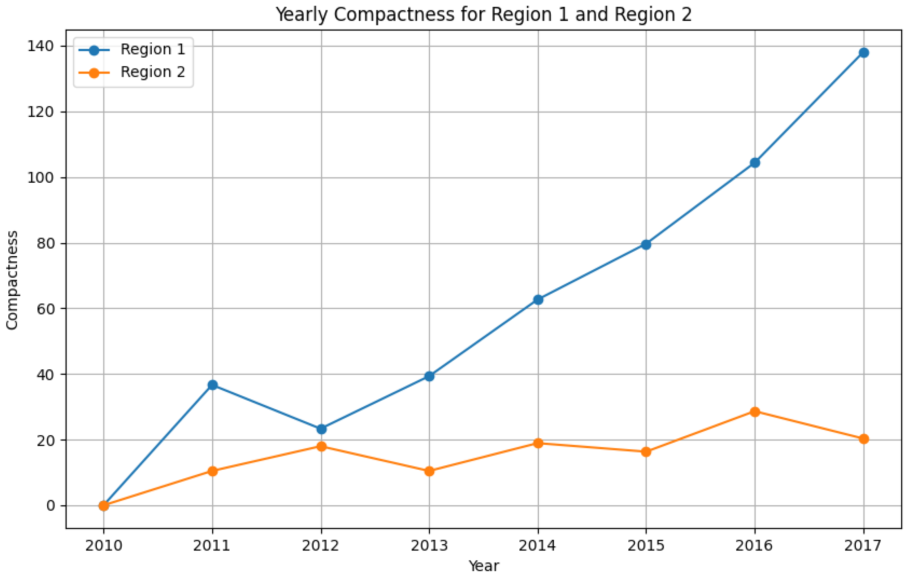
To complement Hamming Distance analysis, we assess yearly compactness scores for both regions, reflecting structural cohesion in disease prevalence. This is shown in Figure 7.
Findings:
  • Region 1: Compactness scores decrease over time, indicating rising disease pattern variability.
  • Region 2: Compactness scores remain relatively stable, reinforcing the consistency of disease trends.
Conclusion: The integration of Hamming Distance, hierarchical clustering, and compactness analysis enhances disease surveillance capabilities, enabling policymakers to design region-specific and adaptive public health strategies.

4.6. Binary Tree Visualization

Binary tree visualizations simplify the interpretation of hierarchical clustering results by offering a structured representation of cluster relationships. While dendrograms provide a comprehensive view of how clusters merge, they become challenging to interpret when dealing with numerous clusters. Binary trees help overcome this limitation by presenting a nested, hierarchical structure that emphasizes key clustering relationships.

4.6.1. Structure and Interpretation of the Binary Tree

The binary tree representation follows the hierarchical clustering process, where
  • Each node represents a cluster of regions grouped based on disease prevalence similarity;
  • Each branch represents a merging event, with earlier merges indicating greater similarity;
  • The depth of a node reflects disease variability, with deeper nodes indicating regions with distinct epidemiological patterns.
The binary tree visualization provides
  • A structured overview of regional clusters based on disease prevalence;
  • A way to identify outliers with distinct disease trends;
  • An intuitive representation of the progression of disease pattern similarity across regions.

4.6.2. Example of Binary Tree Visualization

Figure 8 presents an example of a binary tree derived from the hierarchical clustering process. The tree structure helps in distinguishing groups of regions with closely related disease trends while highlighting regions with unique epidemiological patterns.

4.6.3. Public Health Implications of Binary Tree Analysis

The binary tree visualization offers valuable insights for public health strategy development:
  • Identification of High-Risk Regions: Deep nodes in the binary tree indicate regions where disease trends significantly deviate from others, signaling the need for specialized interventions.
  • Hierarchical Similarity Among Regions: The tree structure highlights regions with closely aligned disease prevalence, allowing for shared intervention strategies.
  • Outlier Detection: Isolated branches or late-merging nodes indicate regions with unique disease patterns, warranting further epidemiological investigation.
Conclusion: The binary tree representation enhances the interpretability of hierarchical clustering results, offering an intuitive way to identify key regional patterns in disease prevalence. This visualization, when combined with dendrograms and Hamming Distance analysis, provides a comprehensive framework for spatial and temporal disease trend analysis.

4.7. Compactness, Depth, and Variability Metrics

To assess the hierarchical structure and consistency of disease patterns within each region, we evaluate clustering results using compactness, depth, and variability metrics.
  • Compactness (C): Compactness measures the overall tightness of clusters and is calculated as
    C = i = 1 n d i n
    where d i represents the distance at which the i-th cluster merges, and n is the total number of clusters.
  • Depth and Variability: Depth quantifies the position of cluster formation within the binary tree, with the root node having a depth of 0. Variability is evaluated using the standard deviation of depth values.

4.7.1. Example Calculation of Depth Metrics

To illustrate depth variability, we provide an example calculation using Dataset 2:
  • Depth Values:  4 , 3 , 4 , 3 , 1 , 2 , 2 , 3 , 1 , 2 , 0
  • Mean Depth ( μ ):
    μ = 4 + 3 + 4 + 3 + 1 + 2 + 2 + 3 + 1 + 2 + 0 11 2.27
  • Standard Deviation ( σ ):
    σ = ( x i μ ) 2 n = 18.96 11 1.31

4.7.2. Comparative Depth and Compactness Analysis

Table 3 presents compactness, depth, and standard deviation metrics for both datasets. These indicators quantify the variability and cohesion of disease prevalence patterns within each region.

4.7.3. Findings and Interpretation

From Table 3, we observe distinct differences in compactness and depth between Dataset 1 and Dataset 2:
  • Dataset 1: A higher compactness score (233.61) and lower average depth (1.91) indicate greater variability in disease prevalence. The deeper nodes—such as Diseases X 4 and X 6 with a depth of 4—suggest that certain diseases follow distinct prevalence trends, requiring more targeted interventions.
  • Dataset 2: A lower compactness score (52.06) and higher average depth (2.27) suggest more stable disease patterns across the region. The more balanced depth values across nodes—such as T 1 , T 2 , and T 3 —indicate that uniform public health measures may be more effective.
The results confirm that Region 1 (Dataset 1) has greater variability in disease patterns, requiring flexible, region-specific interventions. In contrast, Region 2 (Dataset 2) shows more consistent trends, where standardized interventions may suffice.
While these metrics provide insight into the spatial clustering of disease prevalence, they do not account for temporal variability. To address this, the next section integrates Hamming Distance analysis to measure year-over-year disease prevalence shifts.

4.8. Summary of Methodology

This study employs an integrated approach combining hierarchical clustering, Hamming Distance, and binary tree visualization to analyze spatial and temporal patterns of disease prevalence. Applied to regional disease data in Uzbekistan, this framework
  • Identifies natural clusters of regions based on disease prevalence;
  • Tracks year-over-year variability in disease patterns using Hamming Distance;
  • Provides visual insights to aid in public health decision-making.
The next section presents a case study applying this methodology to real-world data, demonstrating its effectiveness in characterizing infectious disease trends.

5. Case Study: Infectious Diseases—Analysis and Results

5.1. Introduction to Infectious Disease Trends

This case study examines infectious disease trends across the regions of Uzbekistan over a 10-year period (2010–2019), excluding the post-2019 period to avoid distortions caused by the COVID-19 pandemic. The analysis aims to identify meaningful patterns in disease prevalence across different economic zones to inform region-specific public health interventions.
Based on the economic classification of regions presented in Table 1, we divided the regions into two groups:
  • Group 1: Industrialized and Less-Developed regions.
  • Group 2: Agricultural and Emerging regions.
The analysis aims to explore whether Industrialized and Less-Developed regions (Group 1) exhibit more fluctuating disease patterns due to urban density and healthcare accessibility, while Agricultural and Emerging (Group 2) regions may show more stable trends. By identifying these patterns, we provide insights into region-specific public health interventions.

5.2. Clustering Insights from Dendrograms

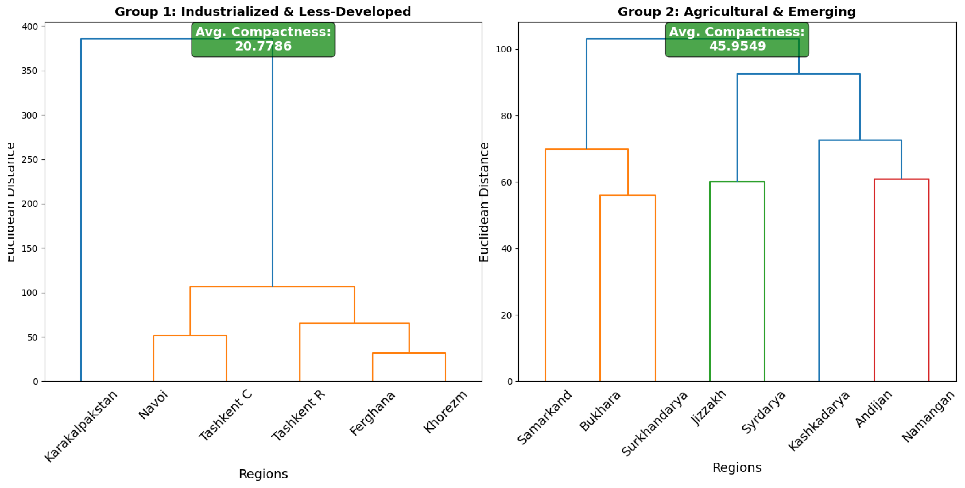
The hierarchical clustering dendrograms for Group 1 and Group 2 reveal distinct patterns in disease prevalence. Differences in cluster structures between the two groups highlight key public health considerations for designing targeted interventions. This is illustrated in Figure 9.

5.2.1. Group 1: Industrialized and Less-Developed Regions

The clustering results for Group 1 indicate a compactness value of 20.78, suggesting that disease patterns exhibit higher variability across these regions.
The dendrogram identifies two major clusters:
  • Cluster 1: Navoi, Tashkent City, and Tashkent region exhibit similar patterns, likely due to shared socio-economic and healthcare factors.
  • Cluster 2: Fergana and Khorezm form a tight subgroup with highly similar health profiles, suggesting shared public health interventions may be effective.
Karakalpakstan stands out as an outlier, merging with the other clusters at a significantly higher distance, indicating distinct disease patterns likely influenced by unique environmental or socio-economic factors.

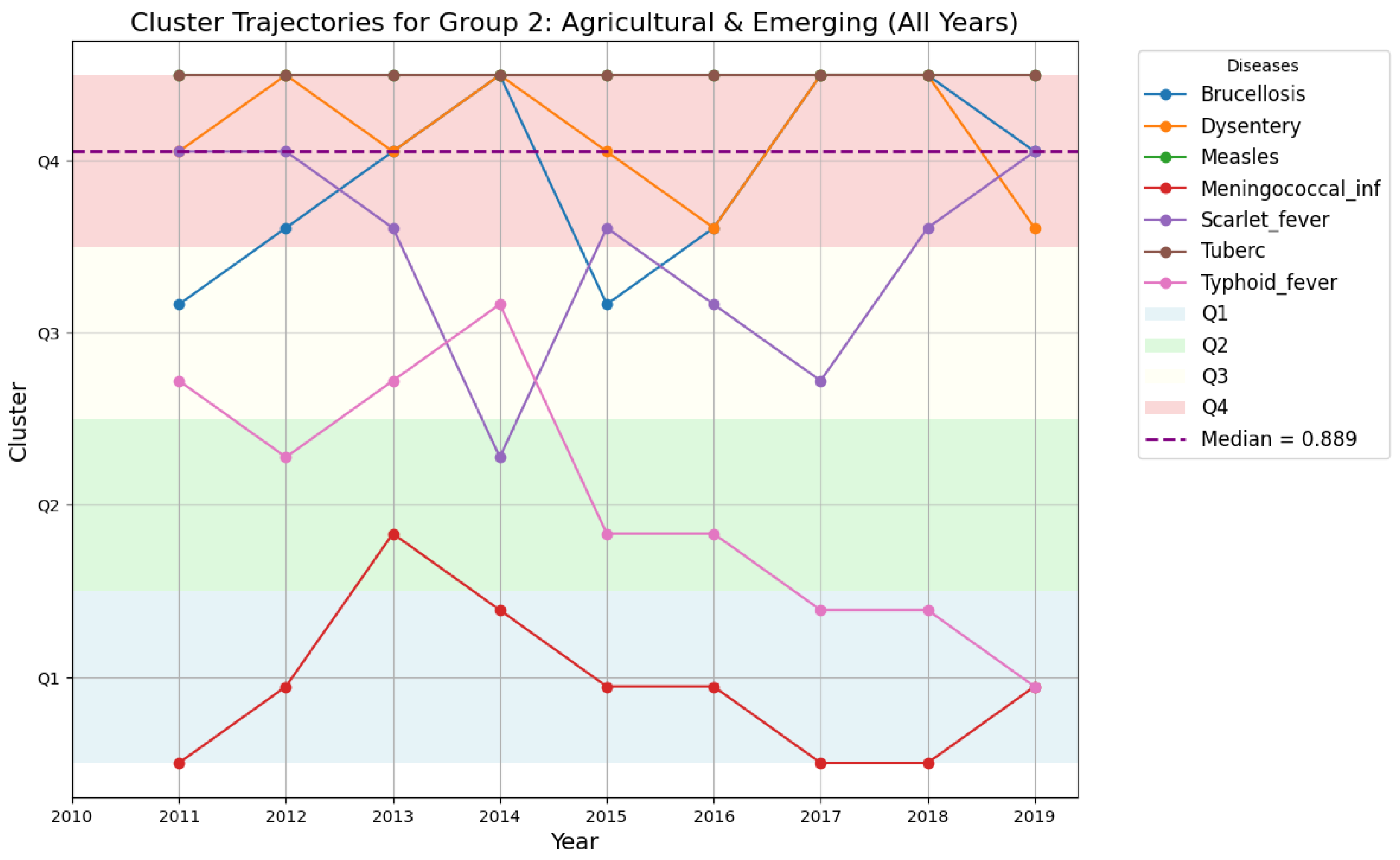
5.2.2. Group 2: Agricultural and Emerging Regions

The compactness value for Group 2 is 45.95, indicating a more cohesive clustering structure compared to Group 1. This suggests that uniform healthcare interventions may be more effective for most regions in this group.
The dendrogram reveals a hierarchical structure:
  • Cluster 1: Samarkand, Bukhara, and Surkhandarya merge at a moderate distance, indicating similar disease trends.
  • Cluster 2: Andijan, Namangan, Kashkadarya, Jizzakh, and Syrdarya form a cohesive cluster. However, Jizzakh and Syrdarya join at a higher distance, suggesting the need for localized adjustments.

5.3. Binary Tree Representation: Simplifying Cluster Interpretation

Binary tree visualizations provide a structured representation of hierarchical clustering results, improving interpretability and outlier detection. This is shown in Figure 10. The corresponding values of depth and compactness are presented in Table 4.
Comparative Depth and Compactness Analysis:
Table 4. Comparative Depth and Compactness Analysis for Group 1 and Group 2.
Group 1Group 2
Node/ClusterDepthNode/ClusterDepth
Karakalpakstan4Samarkand4
Navoi3Bukhara3
Tashkent City3Surkhandarya3
Tashkent Region3Jizzakh3
Fergana2Syrdarya2
Khorezm2Kashkadarya2
Cluster 13Andijan2
Cluster 22Namangan2
Cluster 32Cluster 13
Cluster 41Cluster 22
Cluster 5 (Root)0Cluster 32
Average Depth2.55Average Depth2.33
Standard Deviation1.13Standard Deviation1.07
Compactness24Compactness21

5.4. Hamming Distance Analysis

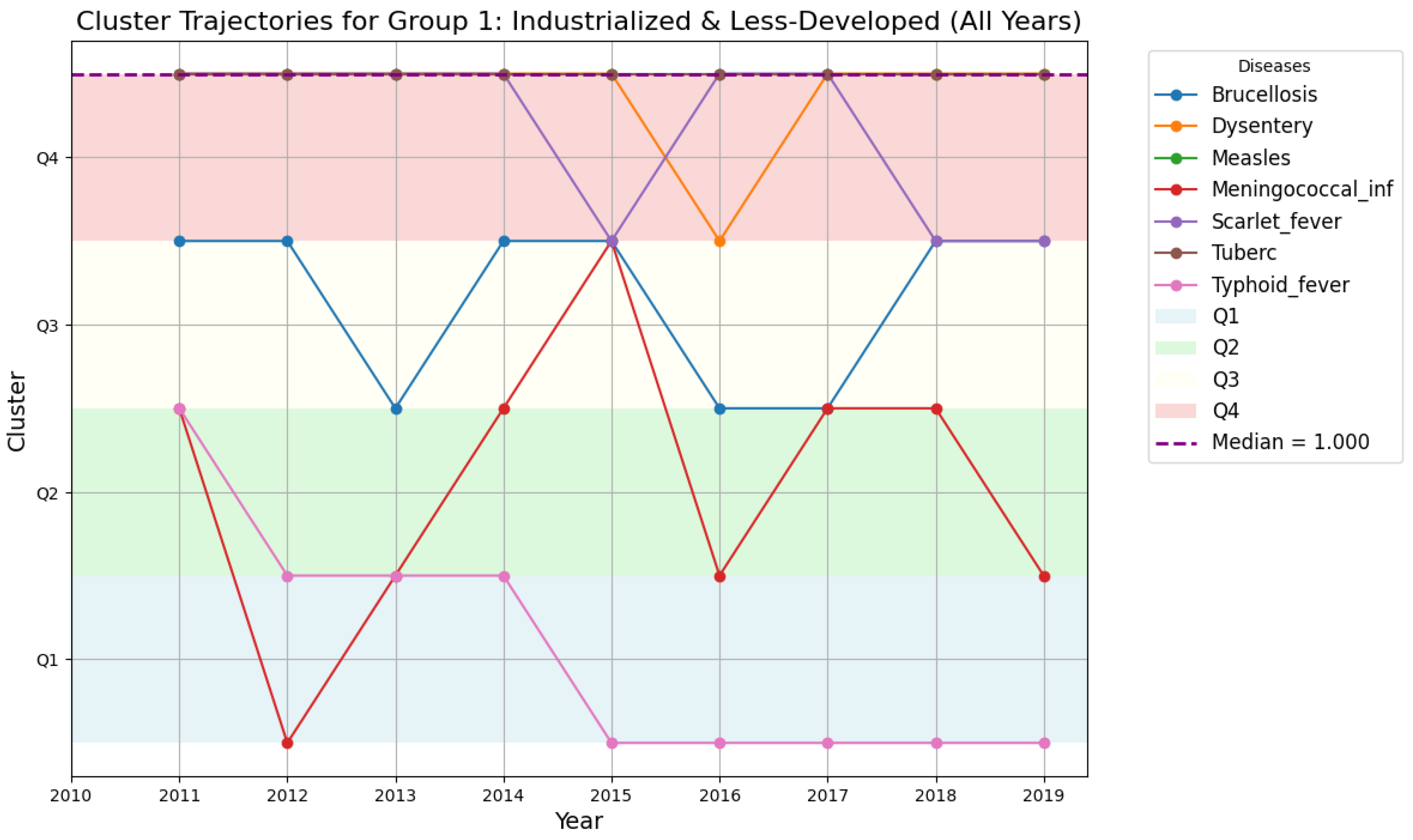
Hamming Distance analysis highlights year-over-year variability in disease prevalence across different regions. The results provide insights into emerging disease patterns that may require targeted intervention. This is shown in Figure 11 and Figure 12.
Key findings from the Hamming Distance analysis are as follows:
  • Group 1: Higher variability in disease patterns, with diseases like Tuberculosis and Dysentery showing consistent year-over-year changes. This suggests that outbreaks in these regions may be strongly influenced by environmental or socio-economic factors, requiring targeted control measures.
  • Group 2: More stable disease patterns, although Measles showed significant fluctuations between 2012 and 2016, suggesting periodic outbreaks that may require vaccination-focused policies.
The analysis highlights key public health implications:
  • Higher Variability in Industrialized Regions: Group 1 shows higher year-over-year variability, indicating the need for region-specific interventions.
  • Stable Patterns in Agricultural Regions: Group 2 exhibits more consistent disease trends, suggesting uniform healthcare policies may be effective.
  • Disease-Specific Trends: Tuberculosis, Dysentery, and Measles demonstrate the highest variability, requiring targeted public health measures.
These findings support a data-driven approach to public health planning, ensuring that resources are allocated based on regional disease dynamics rather than a one-size-fits-all policy.

6. Discussion of Results

The proposed clustering approach is well-suited for analyzing disease patterns in datasets where hierarchical relationships between regions and diseases provide valuable insights. While particularly effective for smaller datasets, it can be extended to broader epidemiological studies across different countries and disease types, provided that at least two years of data are available for at least one disease across multiple regions or cities.
Although this methodology does not uncover the root causes of disease spread, it serves as a powerful tool for tracking spatial and temporal patterns, enabling data-driven public health strategies. Specifically, it facilitates the following:
  • Regional Pattern Identification: Clustering similar regions based on disease progression allows for coordinated health interventions and resource allocation.
  • Detection of Outlier Regions: Identifying regions with unique or irregular disease behaviors supports targeted intervention strategies.
  • Scalability for Comparative Studies: The methodology can be applied to different epidemiological settings, supporting cross-regional and international comparisons of disease trends.
Our results suggest that hierarchical clustering combined with Hamming Distance analysis provides actionable insights into public health trends. By monitoring year-to-year variations in disease prevalence, policymakers can anticipate significant shifts in disease patterns, refine health strategies, and proactively allocate resources to mitigate outbreaks.

Author Contributions

A.A. and E.P. contributed equally to this work. All authors have read and agreed to the published version of the manuscript.

Funding

This research was conducted without any external funding.

Institutional Review Board Statement

Not applicable.

Informed Consent Statement

Not applicable.

Data Availability Statement

Data and code are available at https://github.com/ayau6591/AI_tools_UZ (accessed on 31 July 2025).

Acknowledgments

We thank the Department of Computer Science at Boston University for their support.

Conflicts of Interest

The authors declare no conflicts of interest regarding the publication of this paper.

References

  1. Bamana, A.B.; Kamalabad, M.S.; Oberski, D.L. A systematic literature review of time series methods applied to epidemic prediction. IMU 2024, 50, 10571. [Google Scholar] [CrossRef]
  2. Franch-Pardo, I.; Napoletano, B.M.; Rosete-Verges, F.; Billa, L. Spatial analysis and GIS in the study of COVID-19. A review. Sci. Total Environ. 2020, 739, 140033. [Google Scholar] [CrossRef] [PubMed]
  3. Song, C.; Fang, L.; Xie, M.; Tang, Z.; Zhang, Y.; Tian, F.; Wang, X.; Lin, X.; Liu, Q.; Xu, S.; et al. Revealing spatiotemporal inequalities, hotspots, and determinants in healthcare resource distribution: Insights from hospital beds panel data in 2308 Chinese counties. BMC Public Health 2024, 24, 423. [Google Scholar] [CrossRef] [PubMed]
  4. Ren, Y.; Qian, P.; Duan, Z.; Zhao, Z.; Pan, J.; Yang, M. Disparities in health system input between minority and non-minority counties and their effects on maternal mortality in Sichuan province of western China. BMC Public Health 2017, 17, 750. [Google Scholar] [CrossRef] [PubMed]
  5. Jain, A.K. Data Clustering: 50 Years Beyond K-Means. Pattern Recognit. Lett. 2010, 31, 651–666. [Google Scholar] [CrossRef]
  6. Han, J.; Kamber, M.; Pei, J. Data Mining: Concepts and Techniques, 3rd ed.; Morgan Kaufmann: San Francisco, CA, USA, 2012. [Google Scholar]
  7. Tan, P.N.; Steinbach, M.; Kumar, V. Introduction to Data Mining; Addison-Wesley: Boston, MA, USA, 2006. [Google Scholar]
  8. Porter, M.E. The Economic Performance of Regions. Reg. Stud. 2003, 37, 549–578. [Google Scholar] [CrossRef]
  9. Lai, S.; Farnham, A.; Ruktanonchai, N.W.; Tatem, A.J. Measuring mobility, disease connectivity and individual risk: A review of using mobile phone data and mHealth for travel medicine. J. Travel Med. 2019, 26, taz019. [Google Scholar] [CrossRef] [PubMed]
  10. Anselin, L. Thirty Years of Spatial Econometrics. Pap. Reg. Sci. 2010, 89, 3–25. [Google Scholar] [CrossRef]
  11. Sadeghi, B.; Cheung, R.C.Y.; Hanbury, M. Using hierarchical clustering analysis to evaluate COVID-19 pandemic preparedness and performance in 180 countries in 2020. BMJ Open 2021, 11, e049844. [Google Scholar] [CrossRef] [PubMed]
  12. Pattnaik, S.; Pinsky, E. Hamming Diversification Index: A New Clustering-Based Metric to Understand and Visualize Time Evolution of Patterns in Multi-Dimensional Datasets. Appl. Sci. 2025, 15, 7760. [Google Scholar] [CrossRef]
  13. Brauer, F.; Castillo-Chavez, C.; Feng, Z. Mathematical Models in Epidemiology; Springer: New York, NY, USA, 2019; Volume 32. [Google Scholar]
  14. Skiena, S.S. The Algorithm Design Manual, 2nd ed.; Springer: London, UK, 2012. [Google Scholar]
  15. Cormen, T.H.; Leiserson, C.E.; Rivest, R.L.; Stein, C. Introduction to Algorithms, 3rd ed.; MIT Press: Cambridge, MA, USA, 2009. [Google Scholar]
  16. Box, G.E.; Jenkins, G.M. Time Series Analysis: Forecasting and Control, revised ed.; Holden-Day: San Francisco, CA, USA, 1976. [Google Scholar]
  17. Hyndman, R.J.; Athanasopoulos, G. Forecasting: Principles and Practice, 2nd ed.; OTexts: Melbourne, Australia, 2018. [Google Scholar]
  18. Aggarwal, C.C. Data Mining: The Textbook; Springer: Cham, Switzerland, 2015. [Google Scholar] [CrossRef]
  19. Hulten, G.; Spencer, L.; Domingos, P. Mining Time-Changing Data Streams. In Proceedings of the 7th ACM SIGKDD International Conference on Knowledge Discovery and Data Mining, San Francisco, CA, USA, 26–29 August 2001; pp. 97–106. [Google Scholar] [CrossRef]
  20. Horne, E.; Tibbie, H.; Sheikh, A.; Tsanas, A. Challenges of Clustering Multimodal Clinical Data: Review of Asthma Subtyping Studies. JMIR Med. Inform. 2020, 8, e16452. [Google Scholar] [CrossRef]
  21. Lee, Y.-P.; Wen, T.-H. Understanding the Spread of Infectious Diseases in Edge Areas of Hotspots: A Spatial Analysis of COVID-19 Clusters in Taiwan. Int. J. Health Geogr. 2023, 22, 5. [Google Scholar] [CrossRef] [PubMed]
  22. Ferguson, N.M.; Cummings, D.A.; Cauchemez, S.; Fraser, C.; Riley, S.; Meeyai, A.; Iamsirithaworn, S.; Burke, D.S. Strategies for Containing an Emerging Influenza Pandemic in Southeast Asia. Nature 2005, 437, 209–214. [Google Scholar] [CrossRef] [PubMed]
  23. Nogueira, S.; Brown, G. On the Stability of Feature Selection Algorithms. J. Mach. Learn. Res. 2018, 18, 1–54. Available online: https://jmlr.csail.mit.edu/papers/volume18/17-514/17-514.pdf (accessed on 1 June 2025).
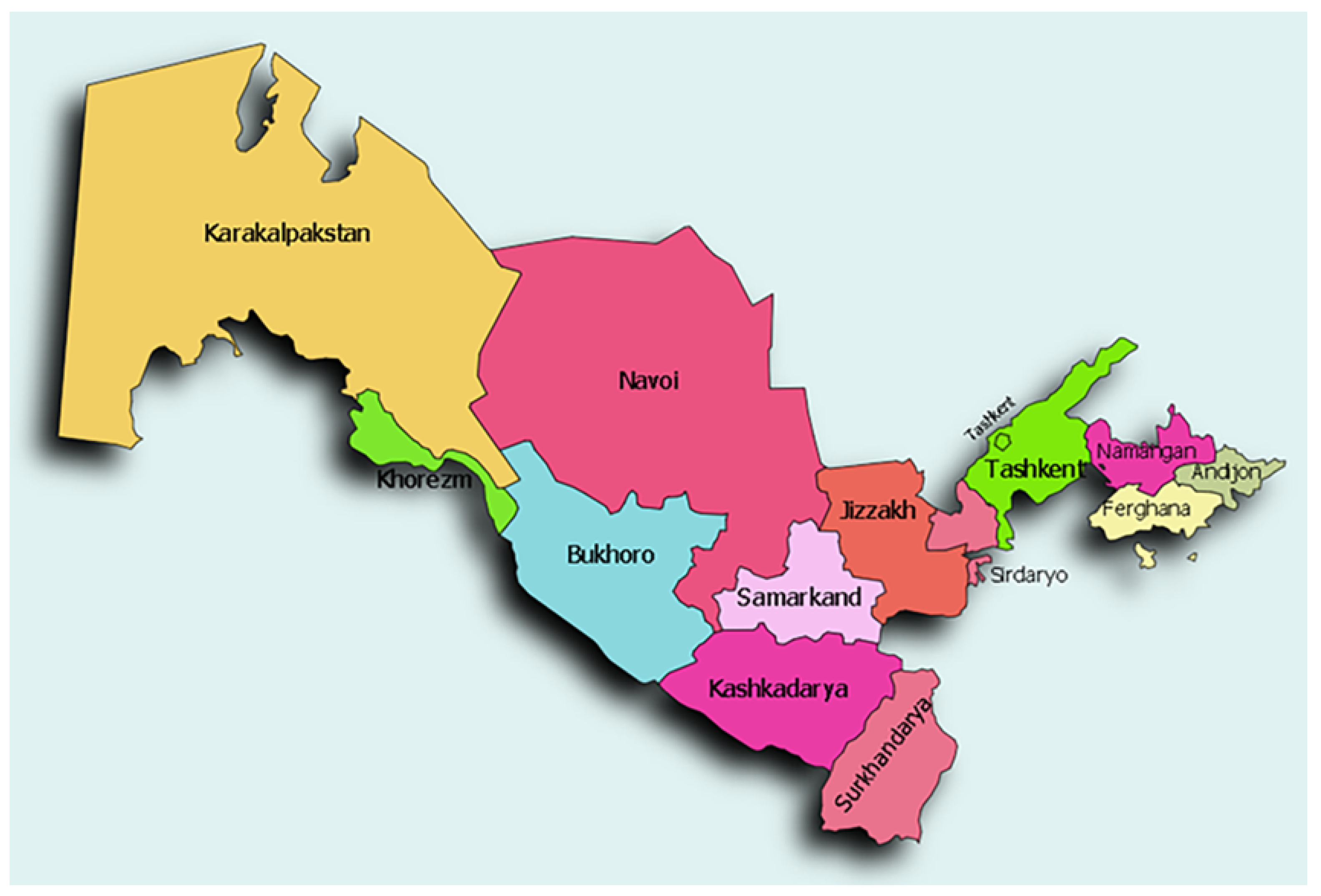
Figure 1. Geographic representation of the 13 regions analyzed in this study. Disease prevalence varies based on population density, climate, and public health interventions in each region.
Csmf 11 00023 g001
Figure 2. Silhouette score and compactness analysis.
Csmf 11 00023 g002
Figure 3. Dendrograms for Region 1 (left) and Region 2 (right).
Csmf 11 00023 g003
Figure 4. Cluster trajectories for Region 1: comparison between the first 4 years (2010–2013) and second 4 years (2014–2017).
Csmf 11 00023 g004
Figure 5. Cluster trajectories for Region 1 and Region 2 (all years: 2010–2017).
Csmf 11 00023 g005
Figure 6. Combined Hamming Distance heatmap for Region 1 and Region 2 (2010–2019).
Csmf 11 00023 g006
Figure 7. Yearly compactness for Region 1 and Region 2 (2010–2017).
Csmf 11 00023 g007
Figure 8. Binary tree visualization for regional clustering.
Csmf 11 00023 g008
Figure 9. Dendrograms for Group 1 and Group 2.
Csmf 11 00023 g009
Figure 10. Binary trees for Group 1 and Group 2.
Csmf 11 00023 g010
Figure 11. Hamming Distance trajectories for Group 1 (2010–2019).
Csmf 11 00023 g011
Figure 12. Hamming Distance trajectories for Group 2 (2010–2019).
Csmf 11 00023 g012
Table 1. Economic and development classification of study regions.
Development GroupEconomic ZoneRegion
Group 1Less DevelopedKarakalpakstan
Less DevelopedKhorezm
IndustrializedNavoi
IndustrializedTashkent R
IndustrializedFergana
IndustrializedTashkent C
Group 2AgriculturalAndijan
AgriculturalNamangan
AgriculturalSurkhandarya
AgriculturalSyrdarya
EmergingBukhara
EmergingJizzakh
EmergingKashkadarya
EmergingSamarkand
Table 2. Summary of notation used in the study.
SymbolDefinition
X i Incidence rate of disease i in Region 1
T i Incidence rate of disease i in Region 2
d H ( X , Y ) Hamming Distance between two time-series X and Y
C k Cluster k identified in hierarchical clustering
μ ( C k ) Mean value of all points in cluster C k
W C S S k Within-Cluster Sum of Squares for cluster k
S k Silhouette score for cluster k
D i j Dissimilarity between two regions i and j
Table 3. Comparative depth and compactness analysis for Dataset 1 and Dataset 2.
Dataset 1Dataset 2
Node/ClusterDepthNode/ClusterDepth
X 1 1 T 1 3
X 2 2 T 2 2
X 3 3 T 3 3
X 4 4 T 4 2
X 5 2 T 5 1
X 6 4 T 6 2
Cluster 13Cluster 12
Cluster 22Cluster 21
Cluster 33Cluster 32
Cluster 42Cluster 41
Cluster 5 (Root)0Cluster 5 (Root)0
Average Depth: 1.91Average Depth: 2.27
Standard Deviation: 1.07Standard Deviation: 1.31
Compactness: 233.61Compactness: 52.06
Disclaimer/Publisher’s Note: The statements, opinions and data contained in all publications are solely those of the individual author(s) and contributor(s) and not of MDPI and/or the editor(s). MDPI and/or the editor(s) disclaim responsibility for any injury to people or property resulting from any ideas, methods, instructions or products referred to in the content.