Abstract
Effective forecasting is vital in various domains as it supports informed decision-making and risk mitigation. This paper aims to improve the selection of appropriate forecasting methods for univariate time series. We propose a systematic categorization based on key characteristics, such as stationarity and seasonality and analyze well-known forecasting techniques suitable for each category. Additionally, we examine how forecasting horizons, the time periods for which forecasts are generated, affect method performance, thus addressing a significant gap in the existing literature. Our findings reveal that certain techniques excel in specific categories and demonstrate performance progression over time, indicating how they improve or decline relative to other techniques. By enhancing the understanding of method effectiveness across diverse time series characteristics, this research aims to guide professionals in making informed choices for their forecasting needs.
1. Introduction
Forecasting, the process of making predictions about future events based on historical data, plays an important role in various fields, including finance [1], supply chain management [2], environmental science [3], etc. Accurate forecasting enables organizations to make informed decisions [4], optimize resources [5], and mitigate risks [6]. As the volume of time series data continues to grow, understanding the aspects of forecasting techniques becomes increasingly critical.
A crucial task in time series forecasting is the identification of the most suitable forecasting method for a dataset containing univariate data [7]. While it may seem convenient to apply a single forecasting method across all time series, research indicates that such an approach is unlikely to produce optimal results universally. Makridakis et al. (1982) [8] demonstrated that no single forecasting method consistently outperforms others across different scenarios, emphasizing the necessity for a more refined approach. Numerous studies have emphasized the importance of selecting appropriate forecasting methods suitable to the characteristics of the data. Therefore, categorizing time series datasets based on their inherent characteristics is essential in determining the most effective forecasting methods for each category.
Some of the characteristics of time series data used in characteristic-based clustering, as identified by Wang et al. (2006) [9], include trend, seasonality, periodicity, serial correlation, skewness, kurtosis, chaos, nonlinearity, and self-similarity. However, conducting a comprehensive analysis across all possible categories is not feasible. The varying degrees and types of these characteristics lead to a vast number of unique combinations, making it challenging to apply and evaluate different forecasting algorithms for each scenario. Therefore, for the categorization of the time series data, we focus on the main characteristics that predominantly affect forecasting accuracy. We first split the time series data into stationary and non-stationary datasets using the Augmented Dickey–Fuller test [10]. Stationary time series datasets exhibit a constant mean, constant variance, constant autocorrelation, no trend, and no seasonality. Next, we analyze the non-stationary data, where we identify seasonality as a key factor significantly influencing prediction accuracy. Therefore, we further categorize the non-stationary data into seasonal and non-seasonal datasets.
Previous studies have largely overlooked the impact of the forecasting horizon, specifically how far into the future predictions are made, on method performance, and this is a gap that this paper aims to address. After proposing the categorization of time series data based on their key characteristics, we apply well-known forecasting algorithms for each category and evaluate their performance across varying forecasting periods. Our ultimate goal is to identify the most suitable methods for accurate and reliable forecasting, ensuring that our analysis reflects the complexities inherent in time series data. The proposed comprehensive approach not only enhances the understanding of which methods are most effective for time series data with varying characteristics but also contributes to the enhancement of forecasting practices in the field.
2. Literature Review
There are various methods and concepts for univariate time series forecasting, ranging from simple statistical techniques such as autoregressive (AR) models, Moving Average, and Exponential Smoothing Methods [11] to complex machine learning approaches such as ARIMA [12], SARIMA [13], support vector regression (SVR) [14], K-nearest neighbors (KNN) [15], decision trees [16], Facebook Prophet [17], Neural Prophet [18], and Long Short-Term Memory (LSTM) networks [19]. The selection of the most appropriate methods depends on the characteristics of the time series data and the desired complexity of the algorithm that will be used. Various approaches for algorithm selection have been proposed, including those by Talagala et al. [20], who utilized meta-learning, and those by Petropulous et al. [21], who investigated how judgment can enhance forecasting model selection.
The evaluation of the performance of the method depends on the accuracy of the prediction as well as on the required effort (computing power and complexity of the algorithms). The accuracy depends on the time interval since, in most cases, longer prediction horizons lead to decreased accuracy. In this paper, we examine the effectiveness of time series forecasting methods, particularly focusing on how accuracy varies over different forecasting horizons.
3. Methodology Review
In this section, we present the proposed classification of the time series data and the forecasting algorithms used in our analysis.
3.1. Classification of Time Series Data
In this study, we classify time series data based on two key characteristics—stationarity and seasonality—as these factors significantly influence the performance of various forecasting methods.
3.1.1. Stationarity
Stationarity is a statistical property of a time series where the mean, variance, and autocorrelation structure remain constant over time, without exhibiting trend or seasonality. To assess stationarity, we use the Augmented Dickey–Fuller (ADF) test, which evaluates the presence of a unit root in the data. The null hypothesis of the ADF test states that the series has a unit root (i.e., it is non-stationary). Key components of the ADF test are the ADF statistic, p-value, and critical values. The ADF statistic is the calculated value from the test; a more negative value indicates stronger evidence against the null hypothesis of non-stationarity. The p-value represents the probability of observing the results under the null hypothesis, with smaller values suggesting stronger evidence against it. Critical values are thresholds at different significance levels (e.g., 1%, 5%, or 10%) for comparison.
We reject the null hypothesis, indicating stationarity, if the p-value is less than or equal to the significance level (e.g., 0.01, 0.05, or 0.10) and the ADF statistic is more negative than the critical value at the chosen significance level. Otherwise, we do not reject the null hypothesis, indicating non-stationarity. In our implementation, we use a significance level of 5% (0.05) for the ADF test. If the p-value exceeds 0.05, we conclude that the series is non-stationary. On the other hand, if the p-value is less than or equal to 0.05, we evaluate the ADF statistic against the critical value at the 5% significance level to determine stationarity.
3.1.2. Seasonality
Next, we analyze non-stationary data for seasonality. Seasonality refers to periodic fluctuations in a time series that occur at regular intervals and can impact forecasting accuracy. Identifying these patterns is crucial for classifying non-stationary datasets as seasonal or non-seasonal, while stationary datasets are inherently non-seasonal by definition.
Classifying time series data directly into seasonal and non-seasonal categories can be challenging due to the inherent complexities and variations within the data. To address this difficulty, we utilize a metric to measure the strength of seasonality, allowing for a more nuanced understanding of the seasonal characteristic present in the time series. This approach is based on the methodology outlined by Wang, Smith, and Hyndman (2006) [9], which utilizes a time series decomposition to assess the strength of seasonality. A time series decomposition can be expressed as follows:
where represents the smoothed trend component, the seasonal component, and the remainder component. We compute the strength of seasonality using the following formula:
A series with a seasonal strength close to 0 indicates almost no seasonality, while a series with strong seasonality will have approaching 1. Additionally, a threshold of can be used to categorize a series as seasonal or non-seasonal.
In our implementation, we utilize Seasonal-Trend decomposition using LOESS (STL) to analyze the seasonal components of the time series. First, we shift values to ensure all observations are positive, and then we find the optimal lambda () for the Box–Cox transformation, which stabilizes variance for multiplicative models. A value of corresponds to a multiplicative decomposition, while results in an additive decomposition. It is important to note that STL decomposition is designed for additive decompositions. By optimizing , we effectively handle both additive and multiplicative decompositions. Finally, we compute the strength of seasonality, , for different periods based on the STL decomposition results.
Ultimately, we categorize the time series data into three groups: stationary, seasonal (for non-stationary data), and non-seasonal (also for non-stationary data). This classification enables us to implement the most appropriate forecasting methods for each category, leading to more reliable predictions.
3.2. Forecasting Algorithms
Initially, we considered all commonly used forecasting algorithms. However, we observed that many of these algorithms tend to produce a constant prediction, which is represented as a flat line when plotted over time. This behavior suggests that these algorithms primarily use the last values to forecast future outcomes, often failing to properly capture the underlying characteristics and dynamics of the data. A more detailed examination of this issue is provided in Appendix B.1. Therefore, we focused our analysis on forecasting algorithms that demonstrate variability and responsiveness to changes over time within the forecasting horizons, which is presented in the following sections.
3.2.1. Linear Regression
Linear regression [22] is a statistical method with the primary objective to find a linear equation that best predicts the dependent variable y based on the independent variables X. The linear regression model can be expressed as follows:
where y is the dependent variable, are the independent variables (features), is the intercept, are the coefficients of the independent variables, and is the error term.
In our analysis, we adopt an autoregressive approach to linear regression, utilizing lagged features from the time series data to capture temporal dependencies, which means that all X variables represent previous values of the dependent variable. By creating these lagged features, we incorporate historical values into our model. The linear regression model is then trained on a training set that consists of these lagged features. For making predictions across multiple forecasting horizons, we implement a rolling window approach. The optimal number of lags is determined through a grid search from a set containing different values.
3.2.2. Support Vector Regression
Support vector regression (SVR) [14] is a technique used for regression tasks, aiming to find a function that deviates at most by a specified margin from the actual target values in the training set. The SVR model can be expressed as follows:
where w is the weight vector, is the feature mapping function, and b is the bias term. Similar to our approach with linear regression, we use lagged features and a rolling window approach. In our analysis, we implement SVR with a radial basis function (RBF) kernel since it performed better than other kernels. We also experimented with different hyperparameters to optimize the model’s performance.
3.2.3. K-Nearest Neighbors
K-nearest neighbors (KNN) [15] is a supervised learning algorithm used for regression and classification tasks. The primary objective of KNN is to predict the value of a dependent variable based on the values of its k-nearest neighbors in the feature space. The KNN regression model is represented as follows:
where denotes the values of the k-nearest neighbors, and k is the number of neighbors considered. In our analysis, we utilize the same autoregressive approach as with linear regression and SVR, and predictions are made based on the values of the nearest neighbors. We also perform hyperparameter tuning to find the optimal value of k and the weight type.
3.2.4. Decision Trees
Decision trees [16] are a supervised learning algorithm that models relationships by splitting data into subsets based on feature values. In our analysis, we adopt the same autoregressive approach as before. To optimize the model, we tune the hyperparameters of the decision tree, such as the minimum samples per leaf and minimum sample split, through a grid search in order to determine the best configuration for the decision tree model.
3.2.5. Facebook Prophet
Facebook Prophet [17] is an open-source forecasting tool designed for producing high-quality forecasts with time series data that may contain missing values, outliers, and seasonal effects. In our analysis, we apply Facebook Prophet directly to the time series data, rather than creating lagged features as we did with previous methods. This is because the model is specifically designed for univariate data, so it simply generates forecasted values for the given test set.
3.2.6. Neural Prophet
Neural Prophet [18] is a forecasting tool that combines the strengths of traditional time series models with neural network capabilities. It is based on the architecture of Facebook Prophet but incorporates deep learning algorithms for improved accuracy. Neural Prophet is trained using a backpropagation algorithm to minimize the error between the predicted and actual values. Similarly to Facebook Prophet, Neural Prophet is applied directly to time series data.
3.2.7. LSTM
The Long Short-Term Memory (LSTM) architecture [19] addresses the exploding and vanishing gradient issues of conventional recurrent neural networks. It features memory cells with three essential gates: the forget gate, which discards long-term information; the input gate, which integrates long-term and short-term information; and the output gate, which passes adjusted values to the next memory cell.
For the implementation, the time series data were standardized and aggregated into sets of 10 values, with mean values calculated. The train–test ratio was set at 9:1 without any data shuffling. The lengths of the training and testing tensors were four times the missing block size. The models were trained using 32 hidden states and 2 layers, with a learning rate of 0.01 and the Adam optimizer. The predicted block of values was calibrated based on the last actual value.
4. Evaluation
This section provides an in-depth evaluation of the forecasting algorithms utilized in our analysis.
4.1. Dataset and Preprocessing
The dataset utilized in this study is derived from the M4 competition, which originally comprises 100,000 time series selected from various domains, including industries, services, tourism, demographics, and more [23]. However, a significant number of these series contained insufficient data points for our experiments. Therefore, we filtered the dataset to include only daily time series with at least 4000 entries. We conducted the Augmented Dickey–Fuller test to classify the data into stationary and non-stationary series. From the stationary series, we selected 10 for the subsequent experiments. Additionally, we computed the strength of seasonality for all non-stationary series, selecting the 10 datasets with the lowest strength of seasonality as non-stationary non-seasonal data and 10 datasets with the highest strength of seasonality as non-stationary seasonal data. To facilitate comparisons, we reset the first data point for all time series to 1 January 2000, which does not impact the results.
4.2. Metrics Used
The two most commonly used metrics for measuring forecasting accuracy are the root mean squared error (RMSE) and mean absolute error (MAE). While MAE provides a straightforward average of absolute errors, RMSE penalizes larger errors more heavily, making it sensitive to outliers. However, when comparing datasets with different scales, such as one dataset with values in the hundreds and another in the thousands, the average RMSE and MAE are significantly influenced by the larger-scale dataset. To address this issue, we use relative RMSE (RRMSE) and relative MAE (RMAE). RRMSE is calculated as follows:
where represents the actual values, represents the predicted values, n is the total number of observations, and is the mean of the actual values. This metric provides an indication of the model’s performance relative to the scale of the data. In the subsequent sections, we present the RRMSE plots, while the RMAE formula and plots can be found in Appendix A.
4.3. Results
We implemented various forecasting algorithms to evaluate their performance across different forecasting periods, specifically measuring the RRMSE for each period. Our analysis focuses on two forecasting horizons: short term, which comprises a few data points, and long term, which encompasses up to 1 year of daily values.
4.3.1. Stationary Data
In Figure 1, we show the RRMSE results for the stationary data. From the analysis of the plots, it is noticeable that linear regression outperforms other algorithms for short-term forecasting, closely followed by decision trees. In contrast, Facebook Prophet, Neural Prophet, and LSTM demonstrate suboptimal performance in this context. Prophet models initialize their predictions based on a fitted trend line, which may not accurately reflect the immediate behavior of the time series, particularly at the beginning of the forecasting horizon. In contrast, the other algorithms leverage recent observations directly, making them more sensitive to local patterns and recent changes in the data. When analyzing long-term forecasting, we observe that decision trees outperform linear regression and other algorithms. It is worth mentioning that Facebook Prophet performs better than KNN and SVR, exhibiting a comparable RRMSE to linear regression at the 365-day mark. In contrast, both KNN and SVR show a deterioration in error over time, ultimately yielding similar errors to Neural Prophet, while LSTM consistently performed the worst for stationary data across most forecasting periods.
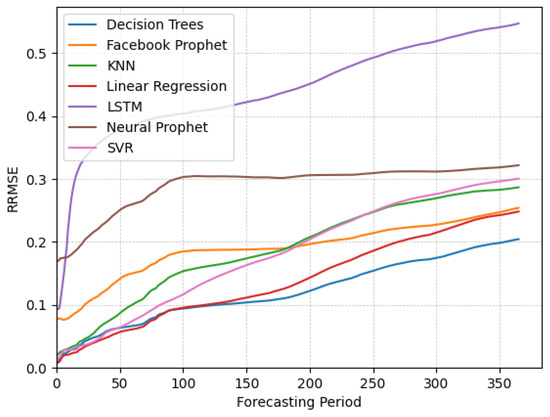
Figure 1.
Plots of RRMSE over time for different algorithms applied on the stationary data.
In Figure 2, we illustrate a forecasting example from one of the 10 datasets used in our analysis of stationary data. In the top plot, we display the actual time series data, with the training data shown in gray and the actual values of the test data in blue. Below that, we present the predictions from the forecasting algorithms under consideration compared to the actual test data. We observe that each algorithm produces distinct prediction patterns; some are able to capture the underlying dynamics accurately, while others do not perform as well.
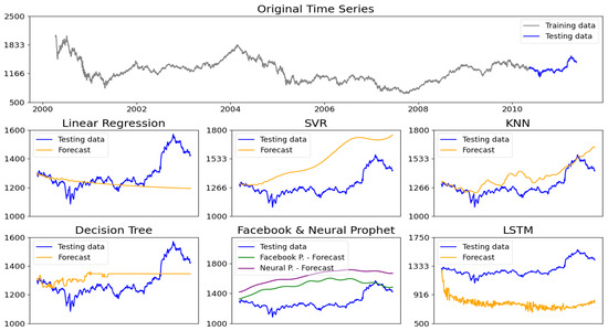
Figure 2.
Comparison of forecasting models on a stationary time series dataset.
4.3.2. Non-Stationary Seasonal Data
In this section, we analyze the forecasting performance of various algorithms on non-stationary seasonal data. As shown in Figure 3, the RRMSE values for seasonal data are higher than those for stationary data. This increase is a result of the particular attributes of the datasets being evaluated, and therefore, direct comparisons with the results from other data categories are not meaningful. For short-term forecasting, our results indicate that decision trees, KNN, and linear regression exhibit better performance relative to the other algorithms. However, we observe that linear regression’s forecasting capabilities deteriorate more over time due to its inability to adequately capture the seasonality present in the data. In contrast, KNN emerges as a more suitable algorithm, demonstrating consistent performance in both short- and long-term forecasts. Interestingly, while SVR initially underperformed in the short term, it ultimately achieved a smaller error than the other algorithms by the end of the forecasting horizon. Given the similar performances of these algorithms, one may choose any of the well-performing options based on additional factors, such as computational efficiency and ease of implementation.
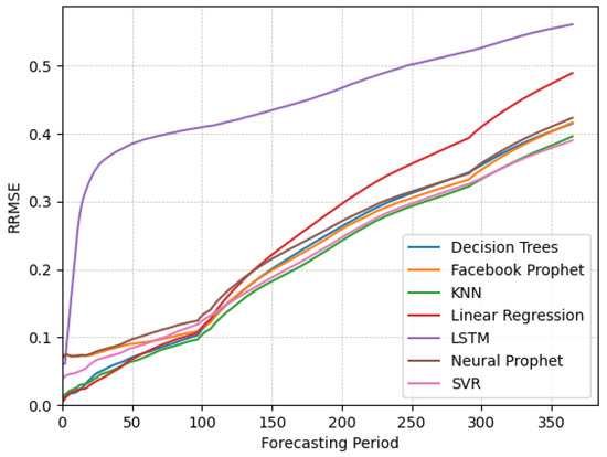
Figure 3.
Plots of RRMSE over time for different algorithms applied on the seasonal data.
In Figure 4, we present a forecasting example from one of the 10 datasets utilized for seasonal data. Each algorithm generates unique prediction patterns as they attempt to effectively capture the seasonality inherent in the dataset. Out of these, KNN is the algorithm that most closely matches the shape and actual values. This is due to KNN’s ability to imitate the patterns in the data by leveraging the k-nearest neighbors from past values.
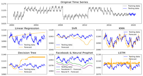
Figure 4.
Comparison of forecasting models on a non-stationary seasonal time series dataset.
4.3.3. Non-Stationary Non-Seasonal Data
Lastly, we evaluate the forecasting performance of various algorithms on non-stationary non-seasonal data. As illustrated in Figure 5, it is evident that linear regression consistently yields the lowest error across all periods, indicating its effectiveness in capturing the patterns within the non-stationary non-seasonal data. Decision trees, KNN, and SVR also demonstrate competitive performance, particularly in the short-term forecasts, maintaining an error significantly lower than other algorithms.
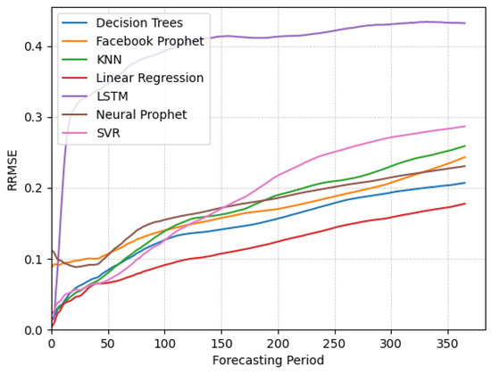
Figure 5.
Plots of RRMSE over time for different algorithms applied on the non-seasonal data.
However, we observe that SVR struggles to capture data complexities for long-term forecasting, as indicated by its relatively higher RRMSE values throughout the forecasting period. Both Facebook Prophet and Neural Prophet demonstrate inadequate performance, particularly in the initial forecasting periods, where they fail to adapt quickly to changes in the data. Additionally, KNN shows a decline in forecasting ability over time compared to other algorithms. Overall, linear regression and, to some extent, decision trees appear to be the most suitable algorithms for forecasting non-stationary non-seasonal data, effectively adapting to the underlying patterns. In contrast, LSTM consistently exhibits the worst performance, similar to its performance in both stationary and non-stationary seasonal data.
In Figure 6, we illustrate a forecasting example from one of the datasets categorized as non-seasonal. We find that linear regression is particularly effective in predicting the overall trend in the data. However, it achieves this by producing a relatively straight line, which means it does not account for any fluctuations or variations present in the dataset. This characteristic allows linear regression to provide a clear representation of the trend, but it may overlook important short-term changes.
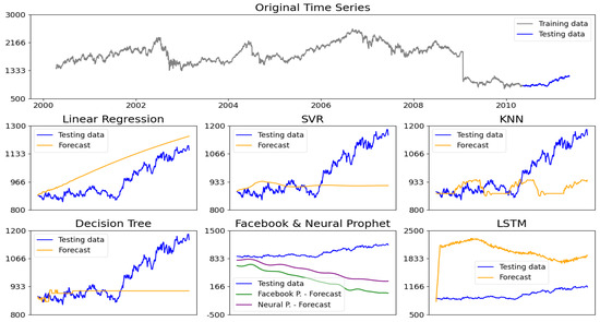
Figure 6.
Comparison of forecasting models on a non-stationary non-seasonal time series dataset.
4.3.4. Running Time Comparison
In this section, we show the computational efficiency of the forecasting algorithms. The algorithms were executed on the stationary data, consisting of 10 datasets each containing around 4200 data points. The experiments were conducted on a CPU with the following specifications: Intel® Core™ i7-10850H (12 Cores, 2.70 GHz, 16 GB RAM). The running time for each algorithm is measured in seconds, and the results are summarized in Table 1.

Table 1.
Running time of forecasting algorithms.
The results of the running time analysis reveal notable differences in computational efficiency among the forecasting algorithms. As expected, linear regression is the fastest algorithm due to its straightforward mathematical model. In contrast, more complex algorithms such as Neural Prophet and Long Short-Term Memory (LSTM) networks demonstrate significantly longer execution times.
These neural network-based approaches have complex structures that require significant processing power, leading to longer runtimes. Algorithms such as SVR, KNN, and decision trees also exhibit moderate running times, making them notably faster than the neural network methods, while Facebook Prophet takes slightly longer than these algorithms. Users must consider the specific requirements of their applications when selecting an appropriate forecasting method. We discuss practical considerations and the limitations of our approach in Appendix B.2 and Appendix B.3.
5. Conclusions
In summary, this paper aims to bridge the gap in the existing literature by systematically categorizing univariate time series data and analyzing the performance of various forecasting algorithms across varying forecasting horizons. The evaluation of various forecasting algorithms revealed significant differences in accuracy and computational efficiency across different types of time series data. For stationary datasets, linear regression outperformed other methods in short-term forecasting and was the fastest overall. In long-term forecasting, decision trees showed superior performance. For non-stationary seasonal data, KNN emerged as the most effective algorithm, demonstrating consistent performance in both short- and long-term forecasts. For non-stationary non-seasonal data, linear regression again ranked as the most effective. In contrast, complex models like LSTM and Neural Prophet struggled to capture time series dynamics, resulting in lower accuracy and higher computational runtime. This work provides valuable insights that can help professionals in selecting the most appropriate forecasting methods for their specific applications.
Author Contributions
Conceptualization, L.D. and G.B.; methodology, L.D.; validation, L.D.; formal analysis, L.D. and A.R.; investigation, L.D.; data curation, L.D.; writing—original draft preparation, L.D.; writing—review and editing, G.B. and A.R.; visualization, L.D. and A.R. All authors have read and agreed to the published version of the manuscript.
Funding
This paper was funded by Fraunhofer Society and the German Federal Ministry for Economic Affairs and Energy.
Institutional Review Board Statement
Not applicable.
Informed Consent Statement
Not applicable.
Data Availability Statement
The original data used in the study are openly available in the M4 competition GitHub repository at https://github.com/Mcompetitions/M4-methods/tree/master/Dataset (access on 5 August 2025).
Conflicts of Interest
The authors declare no conflicts of interest.
Appendix A. RMAE Results
This section provides the formula for the relative mean absolute error (RMAE) and includes corresponding plots to illustrate the RMAE results, as was carried out for RRMSE. RMAE is calculated as follows:
This metric measures the average absolute error between the predicted and actual values, normalized by the mean of the actual values. By using both RRMSE and RMAE, we ensure a meaningful comparison of forecasting performance across datasets with varying scales. The RMAE results exhibit similar shapes throughout the forecasting periods compared with the RRMSE. Figure A1, Figure A2 and Figure A3 below illustrate the RMAE performance for different data categories.

Figure A1.
Plots of RMAE over time for different algorithms applied on the non-seasonal data.

Figure A2.
Plots of RMAE over time for different algorithms applied on the non-stationary seasonal data.

Figure A3.
Plots of RMAE over time for different algorithms applied on the non-stationary non-seasonal data.
Appendix B. Discussion
Appendix B.1. Omission of Certain Algorithms
In our analysis, we observed that certain algorithms, such as polynomial regression, tended to produce forecasts that extended beyond reasonable bounds when predicting further into the future. Additionally, we explored other forecasting methods, including GARCH and Transformers. However, initial experiments yielded unsatisfactory results, which led us to exclude these algorithms from our analysis.
In addition, we noted that algorithms like Random Forest, Gradient Boosting, Exponential Smoothing, ARIMA, and SARIMA exhibited a tendency to converge to a flat (horizontal) line after the initial predictions. Although these methods may demonstrate superior performance in certain scenarios when compared to the performance of other algorithms based on the metrics we employed, their predictions do not accurately reflect the underlying dynamics of the time series data. This limitation ultimately influenced our decision to exclude these algorithms from the preceding analysis.
Appendix B.2. Practical Considerations
The choice of forecasting algorithm should be adjusted to the specific characteristics of the dataset and the forecasting horizon. Users should prioritize algorithms like linear regression or decision trees for applications requiring quick and accurate forecasts. For datasets with complex seasonal patterns, KNN and SVR may provide robust alternatives, especially when long-term adaptability is a concern. By understanding the strengths and limitations of each method, users can make informed decisions, leading to more reliable and effective forecasting outcomes.
Appendix B.3. Limitations of Our Approach and Future Research Directions
While our study provides valuable insights, it is not without limitations. One significant limitation is that we primarily focused on stationarity and seasonality as the key characteristics of the time series data influencing the forecasting capabilities of the models. However, other characteristics, such as trend and skewness can also significantly affect forecasting performance.
Future research could explore the integration of hybrid models that combine the strengths of various algorithms, potentially enhancing forecasting performance across diverse datasets. Additionally, applying these methods to real-world scenarios with varying data characteristics could provide further validation of our findings.
References
- Sezer, O.B.; Gudelek, M.U.; Ozbayoglu, A.M. Financial time series forecasting with deep learning: A systematic literature review: 2005–2019. Appl. Soft Comput. 2020, 90, 106181. [Google Scholar] [CrossRef]
- Raiyani, A.; Lathigara, A.; Mehta, H. Usage of time series forecasting model in Supply chain sales prediction. IOP Conf. Ser. Mater. Sci. Eng. 2021, 1042, 012022. [Google Scholar] [CrossRef]
- Bărbulescu, A. Studies on Time Series Applications in Environmental Sciences; Springer: Berlin/Heidelberg, Germany, 2016. [Google Scholar]
- Tilman, A.; Vasconcelos, V.; Akçay, E.; Plotkin, J. The evolution of forecasting for decision-making in dynamic environments. Collect. Intell. 2023, 2, 26339137231221726. [Google Scholar] [CrossRef]
- Datta, S.; Graham, D.P.; Sagar, N.; Doody, P.; Slone, R.; Hilmola, O.P. Forecasting and Risk Analysis in Supply Chain Management: GARCH Proof of Concept. In Managing Supply Chain Risk and Vulnerability: Tools and Methods for Supply Chain Decision Makers; Springer: London, UK, 2009; pp. 187–203. [Google Scholar] [CrossRef]
- Lu, X. A Human Resource Demand Forecasting Method Based on Improved BP Algorithm. Comput. Intell. Neurosci. 2022, 2022, 3534840. [Google Scholar] [CrossRef] [PubMed]
- Fatima, S.S.W.; Rahimi, A. A Review of Time-Series Forecasting Algorithms for Industrial Manufacturing Systems. Machines 2024, 12, 380. [Google Scholar] [CrossRef]
- Makridakis, S.; Andersen, A.; Carbone, R.; Fildes, R.; Hibon, M.; Lewandowski, R.; Newton, J.; Parzen, E.; Winkler, R. The accuracy of extrapolation (time series) methods: Results of a forecasting competition. J. Forecast. 1982, 1, 111–153. [Google Scholar] [CrossRef]
- Wang, X.; Smith, K.; Hyndman, R. Characteristic-based clustering for time series data. Data Min. Knowl. Discov. 2006, 13, 335–364. [Google Scholar] [CrossRef]
- Diebold, F.X.; Rudebusch, G.D. On the Power of Dickey-Fuller Tests Against Fractional Alternatives. Econ. Lett. 1991, 35, 155–160. [Google Scholar] [CrossRef]
- Martens, A.; Vanhoucke, M. Integrating corrective actions in project time forecasting using exponential smoothing. J. Manag. Eng. 2020, 36, 04020044. [Google Scholar] [CrossRef]
- Nelson, B.K. Time series analysis using autoregressive integrated moving average (ARIMA) models. Acad. Emerg. Med. 1998, 5, 739–744. [Google Scholar] [CrossRef] [PubMed]
- Dubey, A.K.; Kumar, A.; García-Díaz, V.; Sharma, A.K.; Kanhaiya, K. Study and analysis of SARIMA and LSTM in forecasting time series data. Sustain. Energy Technol. Assess. 2021, 47, 101474. [Google Scholar] [CrossRef]
- Awad, M.; Khanna, R.; Awad, M.; Khanna, R. Support vector regression. In Efficient Learning Machines: Theories, Concepts, and Applications for Engineers and System Designers; Apress: Berkeley, CA, USA, 2015; pp. 67–80. [Google Scholar]
- Taunk, K.; De, S.; Verma, S.; Swetapadma, A. A brief review of nearest neighbor algorithm for learning and classification. In Proceedings of the 2019 IEEE International Conference on Intelligent Computing and Control Systems (ICCS), Madurai, India, 15–17 May 2019; pp. 1255–1260. [Google Scholar]
- Breiman, L. Classification and Regression Trees; Routledge: Abingdon, UK, 2017. [Google Scholar]
- Taylor, S.J.; Letham, B. Forecasting with Facebook Prophet. Am. Stat. 2018, 72, 37–45. [Google Scholar] [CrossRef]
- Triebe, O.; Hewamalage, H.; Pilyugina, P.; Laptev, N.; Bergmeir, C.; Rajagopal, R. Neuralprophet: Explainable forecasting at scale. arXiv 2021, arXiv:2111.15397. [Google Scholar] [CrossRef]
- Hochreiter, S.; Schmidhuber, J. Long short-term memory. Neural Comput. 1997, 9, 1735–1780. [Google Scholar] [CrossRef] [PubMed]
- Talagala, T.S.; Hyndman, R.J.; Athanasopoulos, G. Meta-learning how to forecast time series. Monash Econom. Bus. Stat. Work. Pap. 2018, 6, 16. [Google Scholar] [CrossRef]
- Petropoulos, F.; Kourentzes, N.; Nikolopoulos, K.; Siemsen, E. Judgmental selection of forecasting models. J. Oper. Manag. 2018, 60, 34–46. [Google Scholar] [CrossRef]
- Su, X.; Yan, X.; Tsai, C.L. Linear regression. Wiley Interdiscip. Rev. Comput. Stat. 2012, 4, 275–294. [Google Scholar] [CrossRef]
- Makridakis, S.; Spiliotis, E.; Assimakopoulos, V. The M4 Competition: 100,000 time series and 61 forecasting methods. Int. J. Forecast. 2020, 36, 54–74. [Google Scholar] [CrossRef]
Disclaimer/Publisher’s Note: The statements, opinions and data contained in all publications are solely those of the individual author(s) and contributor(s) and not of MDPI and/or the editor(s). MDPI and/or the editor(s) disclaim responsibility for any injury to people or property resulting from any ideas, methods, instructions or products referred to in the content. |
© 2025 by the authors. Licensee MDPI, Basel, Switzerland. This article is an open access article distributed under the terms and conditions of the Creative Commons Attribution (CC BY) license (https://creativecommons.org/licenses/by/4.0/).