Abstract
Demand forecasting is different from traditional forecasting because it is a process of forecasting multiple time series collectively. It is challenging to implement models that can generalise and perform well while forecasting many time series altogether, based on accuracy and scalability. Moreover, there can be external influences like holidays, disasters, promotions, etc., creating drifts and structural breaks, making accurate demand forecasting a challenge. Again, these external features used for multivariate forecasting often worsen the prediction accuracy because there are more unknowns in the forecasting process. This paper attempts to explore effective ways of leveraging the exogenous regressors to surpass the accuracy of the univariate approach by creating synthetic scenarios to understand the model and regressors’ performances. This paper finds that the forecastability of the correlated external features plays a big role in determining whether it would improve or worsen accuracy for models like ARIMA, yet even 100% accurately forecasted extra regressors sometimes fail to surpass their univariate predictive accuracy. The findings are replicated in cases like forecasting weekly docked bike demand per station every hour, where the multivariate approach outperformed the univariate approach by forecasting the regressors with Bi-LSTM and using their predicted values for forecasting the target demand with ARIMA.
1. Introduction
Time series forecasting has crucial applications in the demand planning and supply chain management area. Among the four steps of demand planning—goal determination, data gathering, demand forecasting, and communicating and synchronizing supply with demand—demand forecasting is the most crucial part because it explicitly determines control variables like demand variability and demand volume that have potential influence [1]. However, the biggest hindrance here is the scale of forecasting hundreds or thousands of different time series with diverse characteristics. For example, a supermarket can have thousands of products in thousands of stores; an energy provider company can have millions of customers in several locations where they provide their services; a car rental company can have many cars in many stations, with each product store combination having different time series characteristics; and so on. It is impossible to draw individual attention to demand forecasting for every single product store combination on a larger scale. Therefore, the forecasting solution has to have an overarching standard collective accuracy rather than performing well in only certain cases but performing badly as a whole. Reliable and precise forecasts are the key to optimising inventory, reducing costs, and improving customer satisfaction because they allow businesses to plan and conduct their day-to-day activities smoothly and efficiently. However, external events can cause hindrances to forecast accuracy. Various factors, such as promotions, holidays, hazards, pandemics, recessions, or even something insignificant, can greatly spike or shrink the demand for certain items in certain locations. As not everything can be predicted in nature, this challenge will likely persist forever. On top of that, it is often difficult to include these external factors, resulting in better accuracy with the multivariate forecasting approach when values for their forecast horizon are also unknown. Thus, the other challenge is to pick the correct external variables in such a way that they can enhance overall prediction accuracy.
There have been various attempts to predict time series with various techniques, but few have taken place in the context of demand planning, and fewer are specific to the leverage of external features. Among those few, Olivares et al. have extended the NBEATS model with the inclusion of exogenous regressors called NBEATSx, which improved the forecast accuracy by almost 20% and by up to 5% over statistical and machine learning models by MAE, rMAE, sMAPE, and rRMSE [2]. Ekambaram et al. analysed exogenous variables with generative models with a wide variety of datasets, but not for forecasting demand [3]. Alhussein et al. proposed a hybrid model named CNN-LSTM, which used CNN for feature extraction and LSTM for sequential learning, using holidays and days of the week as external features to predict hourly electricity demand. Their results are evaluated by a percentage decrease of MAPE by 4.01%, 4.76%, and 5.98% improvement for one, two, and six look-forward time steps [4]. Anggraeni et al. conducted another multivariate demand forecast for Muslim kids clothes based on external events like eid festivals and the months before and after that with ARIMA and ARIMAX. Their ARIMAX model performed better than univariate ARIMA [5], but the time series was singular. Kim et al. used a linear regression to predict demand for refrigerators, television, and smartphones using the lifetime-installed base (IBL) and mean age of the installed base in period t as regressors [6]. Gur Ali and Pinar evaluated their proposed “Two-Stage Information Sharing” forecasting method with an extensive dataset entailing 363 stores and seven product categories from the largest retailer of Turkey with 1 to 12 months forecasting lead time. They have only used marketing as an external variable [7]. Castilho used ARIMA and Support Vector Machine, Random Forest, and XGBoost using season, holiday, temperature, humidity, wind speed, and TV advertising as external drivers, and evaluated three public datasets focused on bike sharing, sales, and insurance. Their research showed a great improvement in the RMSE error measure, but they were tested on a single time series where the demand planning context was missing, the forecast horizon was known for the external signals, and other error measures like MAE were ignored [8]. Lim et al. proposed the temporal fusion transformer (TFT) model with their work from Google Cloud AI Research and tested multi-horizon forecasting on various sectors like electricity, traffic, retail, and volatility. They forecasted retail and volatility with multivariate forecasting and showed that TFT outperforms DeepAR, CovTrans, Seq2Seq, and MQRNN by probability percentiles of P50 and P90. But different granularities were not tested and error metrics like RMSE, MAE, and MAPE were ignored [9]. All of these studies are based on certain scenarios or datasets and are not generalizable, and most of them have made the future forecast horizon known for the external events or exogenous regressors, whereas that is not possible in real world cases.
Thus, this paper aims to explore multivariate demand forecasting in detail with ARIMA models, keeping the future horizons unknown for the exogenous regressors, and evaluating the prediction results with Mean Absolute Error. The model ARIMA, which is implemented with the ‘autoarima’ function from Python’s pmdarima library (version==1.8.3), was chosen because it has demonstrated superior performance in demand forecasting in comparison to other models [10]. The ‘auto-arima’ process seeks to identify the optimal parameters, and implicitly incorporates lagged values through the autoregressive and moving average components for an ARIMA model for each time series among many [11]. The metric MAE is chosen because it is the most suitable for evaluating average forecasting performance, as the positive and the negative errors do not cancel each other out, unlike the phenomenon that occurs when averaging many time series prediction errors in metrics like RMSE. Also, extreme errors are not penalised in MAE due to sensitivity towards outliers like MAPE or MSE [12]. It also enables the stakeholders to gain a clear perspective of how many units they might fall short of or exceed the required demand amount.
2. Materials and Methods
A real-world event can be a result modified by many other events, and those other events can be the result of some other events. Since such omniscience cannot be achieved by humans, we do not have any control over real-world environments. Thus, to understand the events and their inter-correlations better, we created simulated scenarios and events over which we have full control. Therefore, we will try to discover patterns and interpret useful insights from synthetic scenarios with controlled experiments. For the subsequent case study, we will collect the data, preprocess it, and evaluate our synthetic findings by forecasting demand.
2.1. Dataset Creation
For this experiment, we have created a collection of 10 datasets containing 16 series each, separated by a unique identifier, developed to aid case studies and to understand the effects of exogenous regressors. It is specifically introduced to dive deeper into multiple levels of internally modelled exogeneity and to find out the effects of different correlation measures for exogenous regressors with the target variable. In these datasets, the time series are constructed with an internal mix of 16 fixed sets of exogenous regressors, as shown in Figure 1, each with one of the following characteristics:
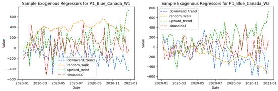
Figure 1.
Samples from 16 fixed sets of exogenous regressors.
Upward Trend:
Downward Trend:
Sinusoidal:
Random Walk:
where is the generated time series value at time t, m is the trend slope, A is the seasonal amplitude, P is the seasonal period, and is the noise term, where . We generate 10 datasets containing 16 series. Each is carried out by choosing each regressor set with fixed coefficient values of 1, 0.75, 0.5, and 0.25. The target value (e.g., Quantity) here is constructed by combining four fixed exogenous regressors, each of which is generated with Equations (1)–(4).
where , , , , are coefficients for the four fixed regressors, respectively. All the are from 16 fixed sets of regressors and is any randomly selected series from (1) to (4). We generated 10 different datasets with 16 different time series generated from each of the 16 fixed regressor sets for daily use with Quantity as the target variable. The datasets were then granulated in weekly formats for further experiments. Samples of them are portrayed in Figure 2.
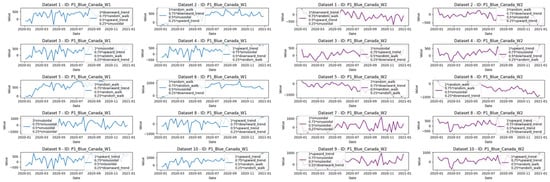
Figure 2.
Example of 10 series generated in each datasets using the sample regressor sets.
The different signals were then further assessed for forecastability using different metrics. The average forecastability scores of all these signals using various metrics are listed in Table 1:

Table 1.
Exogenous forecastability scores for weekly granularity.
Higher values create a more predictable signal for most of the metrics. For sample entropy and coefficient of variation, the lower the score, the better the predictability. The table shows that the metrics act differently based on the regressors and their results are not uniform, and a regressor marked as highly forecastable by one metric might be deemed not very forecastable using another. We will make a further attempt to find the relevant metric later by assessing the results.
2.2. Dataset: Case Study
Divvy is a popular bike-sharing service in Chicago. It allows users to dock and rent bikes from biking stations across the city. The available dataset in Kaggle contains several datasets, but among those, only the “Divvy Trips 1719.csv” and “Chicago Weather 2017 2022[1].csv” were found to be suitable for representing trip details and weather details, respectively [13]. There was another dataset of bus and rail boarding called “CTA Bus Rail Daily Totals.csv” but it was found to be missing years of data; therefore, it was omitted and added from the Chicago Transit Authority’s website. Among all these dataset features, the hour component from “start time” was merged into the “station_id” and made into a unique_id which determined the number of bikes needed for each station at each hour. Then, the number of trips was counted for each unique_id in a “ride_counts” column.
Other exogenous regressor features as shown in Figure 3 like ‘bus onboarding’, ‘bus train total boarding’, ‘rail boardings’, ‘cloudcover’, ‘dew’, feelslike’, ‘sealevelpressure’, ‘snow’, ‘snowdepth’, ‘solar radiation’, ‘solar energy, ‘temp’, ‘total holidays’, ‘uvindex’, ‘visibility’, ‘windgust’, etc., were found to be correlated with a correlation value of above 0.20.
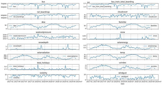
Figure 3.
Correlated exogenous regressors for divyy bike demand forecasting.
Among the 14,614 unique IDs, the unique IDs that had 156 instances of data were segmented as a smooth forecasting sample, which left us a total of 4447 time series with no missing values as shown in Figure 4. While forecasting the bike demand per station each hour, these features and their correlations were further studied by comparison to results from the synthetic datasets and the assessed forecastability of external features is given in Table 2.
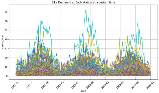
Figure 4.
Divyy bike demand at each hour in each station in Chicago (a total of 4447 time series).
Table 2.
Forecastability scores for bike demand external features.
3. Results
The results for the synthetic dataset before and after the creation of the exogenous regressors known for the future horizon are shown in Table 3.
Table 3.
Exogenous regressor analysis with coefficients, correlations, and MAE values.
Table 3 shows that keeping the forecast horizons unknown for the future horizon often makes the forecasts worse than the univariate forecasting. Also, the regressors that capture the most variance often contribute the most to the prediction accuracy. We can also see that a high correlation does not automatically guarantee the best forecasting performance when used in isolation. In many of the combinations where the predictors or even their sums are used together, the MAE falls significantly. This suggests that the predictors provide complementary information—even the regressor with the lowest individual correlation helps when combined with the others.
From Table 1 we can see that the ARIMA R² Score provides a fairly accurate measurement of how well a standard ARIMA model explains the variance in a series. 1-Permutation Entropy and Sample Entropy provide measures of complexity, but in these cases, the values are very similar for most series, making them less discriminative. Autocorrelation and the Hurst Exponent are informative about persistence and memory in the series, yet they do not capture forecast performance as directly. The Predictability Ratio and Dominant Frequency can be useful in certain settings, but they are not great for the actual multivariate forecasting performance.
Thus, the effectiveness of an exogenous regressor depends on the dataset structure. Sinusoidal and Upward/Downward trends can be great for capturing seasonality or directional trends, but in contrast, Random Walk regressors may work in datasets with high stochasticity but should be used cautiously while forecasting. Also, it is noted that using similar identical regressors additively does not improve prediction accuracy. Poor regressor choices can increase MAE, harming prediction performance.
Looking into the results of Figure 4, we have applied the findings by picking five regressors with different characteristics like ‘railboardings’, ‘cloudcover’, ‘dew’, ‘feelslike’, ‘total holidays’ for the case study. In the case study, the univariate MAE for forecasting bike demand is 1.112. Using all correlated exogenous regressors, keeping their forecast horizons unknown, gives us a worse MAE result of 1.7445. Keeping the forecast horizon unknown for the chosen regressors gives us an MAE of 1.7485. To improve the prediction accuracy of the unknown horizons of the exogenous regressors, we further implemented a Bi-LSTM to predict the future values and used them as exogenous future inputs for the ARIMA model. The B-LSTM model processed time series data using a sliding window approach (look back) to create training sequences, which were then used to train a BiLSTM model with two layers: one with 128 units with return sequences, followed by a second with 64 units without return sequences, both wrapped in bidirectional layers to capture forward and backward temporal dependencies. A dropout layer was included to reduce overfitting, and the model was trained using the Adam optimiser with an MAE loss function and early stopping. The model forecast horizon was scaled using MinMaxScaler and later inverse-transformed for output, with forecasts replicated for each unique ID in the dataset. This resulting MAE using the mix of ARIMA and Bi-LSTM with the five regressors gives us a better MAE result of 1.10, which surpassed our univariate result.
4. Discussion
One of the most significant contributions of this work is its demonstration that exogenous regressors can substantially improve the accuracy of demand forecasts at scale by using two-step or multi-step forecasting. As evident from the synthetic datasets, their performance improvement becomes especially clear when external variables such as holidays, weather patterns, and other situational events are predicted accurately and diverse signals are used. These external features provide valuable context, capturing patterns in demand fluctuations that would otherwise remain unaccounted for if forecasts were solely based on historical data for demand.
The dataset results showed that, particularly for datasets with strong correlation, when the future values of the external regressors were accurate, MAE values dropped in comparison to when only historical data was used. This underscores the importance of precise forecasting of incorporated external variables such as promotions, weather conditions, and economic factors, all of which can lead to sharper predictions in very dynamic environments where demand is influenced by outside events and there is a certain correlation.
While the results are promising, there are still several limitations to this study that should be addressed in future research. First, the synthetic nature of the datasets still limits the direct applicability of these findings to real-world demand forecasting scenarios. Real-world datasets often exhibit noise and irregularities that cannot be captured fully by controlled or determined by any synthetic data, and it remains to be seen how well these results translate into practical settings.
Secondly, we have limited the scope of exogenous variables to a predefined set, excluding other potentially impactful factors such as socioeconomic indicators, market trends, or competition dynamics. Future work might explore the integration of a broader range of external features and assess their impact on forecast accuracy across various industries.
Finally, the evaluation metric (MAE) was selected due to its robustness and interpretability, and the model (ARIMA) was used for scalability and superior performance in the demand-planning scenario, but future studies could benefit from comparing results using other metrics and other models for different multi-step forecasting, enhancing the feature engineering processes, and implementing advanced hyperparameter tuning, particularly in situations where demand is more volatile or extreme. Also, an impact analysis can be conducted to understand how the improved forecasting accuracy translates into tangible benefits for businesses or other stakeholders, both in terms of accuracy and scalability.
5. Conclusions
In conclusion, this study has shown that integrating exogenous regressors into multivariate demand forecasting can lead to substantial improvements in the accuracy of the forecasts. This ability to incorporate external factors like weather, promotions, and holidays can provide the necessary context to make more accurate predictions, especially when these variables are known ahead of time or predicted precisely. However, challenges remain with regard to selecting the correct exogenous features and ensuring that forecasting models can generalise to new, unseen data. Future research should explore ways to incorporate real-world data and handle uncertainty more effectively to create even more reliable multivariate demand forecasting solutions.
Author Contributions
Conceptualization, S.M.A.K. and B.Z.; Methodology, S.M.A.K.; Software, S.M.A.K.; Validation, B.Z. and N.B.L.; Formal Analysis, S.M.A.K., B.Z. and N.B.L.; Investigation, S.M.A.K.; Resources, B.Z.; Data Curation, S.M.A.K.; Writing—Original Draft Preparation, S.M.A.K.; Writing—Review and Editing, S.M.A.K.; Visualization, S.M.A.K.; Supervision, B.Z. and N.B.L.; Project Administration, B.Z.; Funding Acquisition, B.Z. and N.B.L. All authors have read and agreed to the published version of the manuscript.
Funding
This research received necessary computational resources and funding support from Microsoft Development Center Copenhagen and the Department of Digitalisation, Copenhagen Business School.
Institutional Review Board Statement
Not applicable.
Informed Consent Statement
Not applicable.
Data Availability Statement
The publicly available bike sharing data can be found at: https://www.kaggle.com/datasets/leonidasliao/divvy-station-dock-capacity-time-series-forecast. The additional public transport data (bus, rail onboarding) can be found at: https://www.transitchicago.com/ridership/ (accessed on 1 July 2024).
Acknowledgments
I express my sincere gratitude to my Microsoft supervisor Bahram Zarrin and my university supervisor Niels Buus Lassen, from CBS. I feel extremely privileged to have their valuable insights, guidance, critiques, and feedback. Their professional experiences and contributions have sharpened my ideas and kept me motivated. I am forever thankful to them for being great mentors and making this journey rewarding. This work is dedicated to Rehena Akter, who is my mother, a cancer survivor, and a phoenix.
Conflicts of Interest
Author Bahram Zarrin was employed by the company Microsoft. The remaining authors declare that the research was conducted in the absence of any commercial or financial relationships that could be construed as a potential conflict of interest. The authors declare that this study received funding and resource support from Microsoft Development Center Copenhagen and Department of Digitalization, Copenhagen Business School. The funders were not involved in the study design, collection, analysis, interpretation of data, the writing of this article or the decision to submit it for publication.
References
- Swierczek, A. Investigating the role of demand planning as a higher-order construct in mitigating disruptions in the European supply chains. Int. J. Logist. Manag. 2020; ahead-of-print. [Google Scholar]
- Olivares, K.G.; Challu, C.; Marcjasz, G.; Weron, R.; Dubrawski, A. Neural basis expansion analysis with exogenous variables: Forecasting electricity prices with NBEATSx. Int. J. Forecast. 2023, 39, 884–900. [Google Scholar] [CrossRef]
- Ekambaram, V.; Jati, A.; Dayama, P.; Mukherjee, S.; Nguyen, N.H.; Gifford, W.M.; Reddy, C.; Kalagnanam, J. Tiny time mixers (TTMs): Fast pre-trained models for enhanced zero/few-shot forecasting of multivariate time series. arXiv 2024, arXiv:2401.03955. [Google Scholar]
- Alhussein, M.; Aurangzeb, K.; Haider, S.I. Hybrid CNN-LSTM model for short-term individual household load forecasting. IEEE Access 2020, 8, 180544–180557. [Google Scholar] [CrossRef]
- Anggraeni, W.; Vinarti, R.A.; Kurniawati, Y.D. Performance comparisons between ARIMA and ARIMAX method in Moslem kids clothes demand forecasting: Case study. Procedia Comput. Sci. 2015, 72, 630–637. [Google Scholar] [CrossRef]
- Kim, T.Y.; Dekker, R.; Heij, C. Spare part demand forecasting for consumer goods using installed base information. Comput. Ind. Eng. 2017, 103, 201–215. [Google Scholar] [CrossRef]
- Gur Ali, O.; Pinar, E. Multi-period-ahead forecasting with residual extrapolation and information sharing—Utilizing a multitude of retail series. Int. J. Forecast. 2016, 32, 502–517. [Google Scholar] [CrossRef]
- Castilho, C.M. Time Series Forecasting with Exogenous Factors: Statistical vs. Machine Learning Approaches. Master’s Thesis, Universidade do Porto, Porto, Portugal, 2020. AAI30163992. [Google Scholar]
- Lim, B.; Arık, S.; Loeff, N.; Pfister, T. Temporal fusion transformers for interpretable multi-horizon time series forecasting. Int. J. Forecast. 2021, 37, 1748–1764. [Google Scholar] [CrossRef]
- Karim, S.M.A.; Zarrin, B.; Lassen, N. Multivariate Forecasting Evaluation: Nixtla-TimeGPT. In Proceedings of the International Conference on Time Series and Forecasting (ITISE 2025), Gran Canaria, Spain, 16–18 July 2025. (accepted). [Google Scholar]
- pmdarima: ARIMA Estimators for Python. 2017. Available online: http://www.alkaline-ml.com/pmdarima (accessed on 14 April 2025).
- Adhikari, R.; Agrawal, R.K. An introductory study on time series modeling and forecasting. J. Quant. Econ. 2013, 11, 1–15. [Google Scholar]
- Divvy Station Dock Capacity Time Series Forecast. 2022. Available online: https://www.kaggle.com/datasets/leonidasliao/divvy-station-dock-capacity-time-series-forecast (accessed on 1 July 2024).
Disclaimer/Publisher’s Note: The statements, opinions and data contained in all publications are solely those of the individual author(s) and contributor(s) and not of MDPI and/or the editor(s). MDPI and/or the editor(s) disclaim responsibility for any injury to people or property resulting from any ideas, methods, instructions or products referred to in the content. |
© 2025 by the authors. Licensee MDPI, Basel, Switzerland. This article is an open access article distributed under the terms and conditions of the Creative Commons Attribution (CC BY) license (https://creativecommons.org/licenses/by/4.0/).