Abstract
This paper explores the forecasting of aluminum prices using various predictive models dealing with variable uncertainty. A diverse set of economic and market indicators is considered as potential price predictors. The performance of models including LASSO, RIDGE regression, time-varying parameter regressions, LARS, ARIMA, Dynamic Model Averaging, Bayesian Model Averaging, etc., is compared according to forecast accuracy. Despite the initial expectations that Bayesian dynamic mixture models would provide the best forecast accuracy, the results indicate that forecasting by futures prices and with Dynamic Model Averaging outperformed all other methods when monthly average prices are considered. Contrary, when monthly closing spot prices are considered, Bayesian dynamic mixture models happen to be very accurate compared to other methods, although beating the no-change method is still a hard challenge. Additionally, both revised and originally published macroeconomic time-series data are analyzed, ensuring consistency with the information available during real-time forecasting by mimicking the perspective of market players in the past.
1. Introduction
Forecasting commodity prices, particularly aluminum, is essential for producers, consumers, investors, and policymakers. Aluminum is a key material for industries such as construction, aerospace, electronics, and automotive manufacturing. Accurate price forecasting is crucial for making informed decisions regarding investments, production, and trade. However, this is a complex task due to the volatility and unpredictability inherent in commodity markets in general, especially because prices are influenced by various economic, geopolitical, and financial factors, which makes forecasting a very challenging task [1,2,3].
Commodity markets, including aluminum, are affected by supply disruptions, demand fluctuations, geopolitical tensions, and changes in macroeconomic conditions. For example, variations in global industrial production, particularly in major aluminum-consuming countries like China, can significantly affect aluminum demand and prices. Additionally, the claimed financialization of commodities has introduced further complexity, where futures markets and speculative pressures can influence price movements alongside fundamental economic factors [4,5,6]. These dynamics make forecasting commodity prices even more complex, as it requires consideration of both market fundamentals and numerous other factors, leading to model uncertainty or feature selection problems. Furthermore, the relationship between a commodity price and its predictors can vary over time. On the other hand, in many cases, it is difficult to beat the simple no-change (NAIVE) or ARIMA method by generating more accurate forecasts [7,8,9,10,11,12]. Moreover, it is real-time data, which is quickly available to decisionmakers. In contrast, revised data provides a clearer picture of the past, but it is available with a time delay. Constructed models are usually trained using revised data, rather than the one that was truly available to market players in the past. As a result, this can generate another issue in econometric forecasting [13].
A promising approach to the problems above can be obtained through the application of Bayesian dynamic mixture models (BDMMs). These models incorporate model and parameter uncertainty, allowing forecasting adaptation as new information becomes available. However, these methods have not been studied much in applications to commodity prices. Therefore, this study contributes to the literature by comparing the accuracy of forecasts derived from various methods dealing with time-varying parameters and feature selection, as well as originally employing BDMMs in various specifications [14,15]. Furthermore, both real-time and revised datasets are employed.
2. Materials and Methods
2.1. Data
Monthly data from 04/2008 and 10/2024 were analyzed. LME (London Metal Exchange) spot prices (in USD per metric ton; monthly averages) for aluminum (unalloyed primary ingots, high grade, minimum 99.7% purity) were taken from World Bank [16]. This variable was denoted by p_aluminum.
As explanatory variables, excess demand (d_aluminum) was adopted following, for instance, Buncic and Moretto [2]. It was constructed as the difference between global consumption and the sum of global production and inventories. Consumption was proxied from the 2006 global estimates and assumed to mimic the time path of the OECD index of industrial production for China (2015 = 100, calendar and seasonally adjusted), due to a lack of exact data. Indeed, industrial production can be an effective proxy for this variable, and the role of China is huge on the analyzed market [17,18]. Inventories were taken as monthly averages of stocks on LME from Westmetall [19] in thousand metric tonnes. They were also taken as another explanatory variable (stocks_aluminum), as they can proxy speculative pressures. Production was taken in thousand metric tonnes from the International Aluminium Institute [20]. Following Buncic and Moretto [2], a convenience yield (cy_aluminum) was also taken (in percentages). It is constructed as
where r_short is the 3-month risk-free rate (3-month treasury bill: secondary market rate, TB3MS, monthly averages) taken from ALFRED and FRED [21,22], and f_aluminum denotes the official 3-month aluminum prices from LME in USD (^AH_3.F) taken from Stooq [23].
r_short − (f_aluminum − p_aluminum)/p_aluminum,
The US Industrial Production Index (INDPRO) was also taken into account [21,22]. It was denoted by ind_prod. The Index of Global Real Economic Activity (IGREA) proposed by Kilian [24] was obtained from ALFRED and FRED [21,22]. This was denoted by ec_act. Both ind_prod and ec_act were taken as explanatory variables resembling economic conditions.
Market stress was measured by two variables. First, the term spread, denoted by term_spread (i.e., U.S. 10-year treasury constant maturity minus U.S. 2-year treasury constant maturity, T10Y2YM, monthly averages) was used [21,22]. The second, monthly averages of the VIX index of implied volatility [25] were denoted by VIX.
Stock market behavior was measured by the S&P 500 index (^SPX) and the Shanghai Composite Index (^SHC). They were denoted by SP500 and SSE, respectively. This allows for including both the U.S. and Chinese economy—to capture global changes in economies and commodity markets [23]. Additionally, two leading aluminum sector companies’ stock prices were included, i.e., Rio Tinto Plc (RIO.UK, in GBX) and Alcoa Corp (AA.US, in USD), denoted by Rio_Tinto and Alcoa [26,27].
Moreover, two exchange rate currencies to USD of the largest primary aluminum producers were included, i.e., China (USDCNY) and Russia (USDRUB). They were denoted by fx_CNY and fx_RUB, respectively [23,28,29].
Finally, to capture the particular market past or autoregressive behaviors, the World Bank Base Metals Price Index (2010 = 100, USD, including aluminum, copper, lead, nickel, tin, and zinc), denoted by p_metals, was used [16].
Unless otherwise specified, for the above variables, the last observations were always taken into account (and closing and adjusted, if suitable).
2.2. Data Transformations
Similar to, for example, Buncic and Moretto [2], ordinary returns were assumed for most variables. In other words, time-series yt was transformed into (yt − yt−1)/yt where t denotes time. However, cy_aluminum, ec_act, term_spread, and VIX were not differentiated.
Next, following, for example, Koop and Korobilis [30], all variables were standardized into approximately stationary time-series. In other words, yt is a time-series, μ is its mean of the first T observations, and σ is its standard deviation of the first T observations. Then standardization is understood as the transformation of yt = (yt − μ)/σ. In particular, T = 100 was taken (and it was kept throughout the entire study as the in-sample period, for computing forecast accuracy, etc.). A whole sample was not used in order to omit the forward-looking bias. Furthermore, such a transformation allows all the time-series to have similar magnitudes, which improves computational issues in the applied models [31].
However, all forecast evaluation was carried out for raw (levels) aluminum prices; therefore, the predictions of returns obtained directly from the models (except ARIMA, NAÏVE, futures-based, and historical averages, which were computed directly for levels, i.e., raw data) were transformed back into levels. In other words, the estimations of models and their predictions were made over transformed variables, but for evaluation, the predictions of aluminum price were taken.
Explanatory variables were delayed one period back (i.e., first lags), except ec_act, where two periods back (i.e., second lags) were taken. This procedure resembles real-time information availability on the market [21].
Table 1 reports descriptive statistics, and Table 2 shows stationarity tests [32,33,34,35]. When assuming a 5% significance level for all variables, except for cy_aluminum, it can be assumed that they are stationary. Usual tests were applied: augmented Dickey–Fuller (ADF), Phillips–Perron (PP), and (a stationary-level version of) Kwiatkowski–Phillips–Schmidt–Shin (KPSS).

Table 1.
Descriptive statistics.
Table 2.
Stationarity tests.
2.3. Models
As mentioned before, the first 100 observations were taken as in-samples. However, all models were estimated in a recursive manner (i.e., expanding window in-samples), meaning that a forecast for time t was generated from the model trained over all (monthly) data available up to time t − 1.
Firstly, various types of Bayesian dynamic mixture models (BDMMs) were estimated [14,15], both with state-space (SS) and normal regression (NR) components. Besides the original versions, weighted averaging schemes were also modified to include weighted averaged forecasting (A), forecasting from the component model with the highest posterior probability (H), and a median probability model (M) from Barbieri and Berger [36]. These were denoted as BDMM-SS, BDMM-SS-A, BDMM-SS-H, BDMM-SS-M, BDMM-NR, BDMM-NR-H, and BDMM-NR-M [37]. The details can be found in [14,15,37].
Next, Dynamic Model Averaging (DMA), Dynamic Model Selection (DMS), and DMS based on a median probability model (DMP) were estimated. For these models, the standard values of forgetting factors, i.e., 0.99, were taken [38]. Also, Bayesian Model Averaging (BMA), Bayesian Model Selection (BMS), and BMS based on the median probability model (BMP) were estimated. These are versions of the previous models, but with forgetting factors equal to 1. Besides these models, which consider averaging over all possible multilinear regression models (i.e., 2K, where K is the number of explanatory variables, herein K = 14), modified models—averaging over only one-variable simple linear regression models—were also estimated. This is because such models highly reduce computation time, as they consider K + 1 models only (due to the inclusion of a model with constant variable only as well). These were denoted as DMA-1VAR, DMS-1VAR, BMA-1VAR, and BMS-1VAR [39].
Also, LASSO, RIDGE, and Elastic Net (EL-NET) regressions were estimated [40]. Bayesian versions [41] were also estimated (B-LASSO and B-RIDGE). The penalty parameter was selected in a recursive manner (consistently with the spirit of this study) based on t-fold cross-validation (t being the time period) with respect to Mean Square Error (MSE). Mixing parameters {0.1, 0.2, …, 0.9} were applied.
Moreover, the least-angle regression (LARS) was estimated [42] with similar t-fold cross-validation based on MSE.
Additionally, time-varying regressions were estimated (which are equivalent to DMA with only one component model, i.e., the one with constant and all explanatory variables). This was denoted as TVP-FOR. Similarly, time-varying regression with no forgetting was estimated, i.e., the forgetting factor was set equal to 1 (TVP).
The recursively estimated ARIMA model [43] was also used in an automated way, as well as the no-change (NAÏVE) method. Historical-average forecasts were computed both as an expanding window, i.e., including all past historical observations (HA), and as a rolling window of the past 100 periods (HA-ROLL).
Finally, futures-based forecasts were computed [7,44], including the basic ones (FUT-SIMPLE), i.e., futures prices, which are taken directly as the subsequent forecast period, and those based on the spread (FUT-SPREAD).
2.4. Methods
Estimations were carried out in R [45]. The forecast accuracy was measured by Root Mean Square Error (RMSE) and its normalized version (N-RMSE). For N-RMSE, the value of RMSE is divided by the mean of the forecasted time-series. Also, Mean Absolute Error (MAE) and Mean Absolute Scaled Error (MASE) were computed [46]. Competing forecasts were compared pairwise with the Diebold–Mariano test [43,47] with Harvey et al.’s [48] correction method. The full set of forecasts was evaluated with the Model Confidence Set (MCS) from Hansen et al. [49]. Squared error loss functions were applied [50]. Additionally, the Giacomini and Rossi fluctuation test [51] was employed. The rolling parameter μ = 0.6 was used, which corresponds to approximately 5-year periods for the analyzed data [52].
3. Results
3.1. Main Results
Table 3 reports values of forecast accuracy measures. It can be seen that FUT-SPREAD generated the most accurate forecast. Also, FUT-SIMPLE is the second-most accurate forecast. The third best is DMA. This is according to each of the considered metrics. In the case of RMSE or N-RMSE, BDMMs do not perform very well, but if MAE or MASE is applied, BDMM-SS-A seems to be in top positions. Still, futures-based forecasts are the most accurate, DMA places next, and Bayesian versions of penalty regression models follow afterwards.
Table 3.
Forecast accuracy measures.
Table 4 reports outcomes from the Diebold–Mariano test. The forecast from the most accurate model, i.e., FUT-SPREAD, is compared with those from other methods. The same procedure is performed for the most accurate BDMM model, i.e., BDMM-SS-A, and for DMA. Assuming a 5% significance level, it can be seen that in the majority of cases, the competing method can be assumed to be significantly less accurate than FUT-SPREAD, except for FUT-SIMPLE, BDMM-SS-A, and DMA. In the case of the BDMM-SS-A method, only BDMM-SS and historical-average methods can be assumed to be less accurate. In the case of DMA, models such as BDMM-SS-M, BMS-1VAR, and TVP can additionally be assumed to be less accurate. If the absolute scaled error loss function, i.e., the one corresponding to the MASE metric, is considered, then the outcomes are even stronger. All models are less accurate than FUT-SPREAD. In the case of BDMM-SS-A, both time-varying parameter regressions (TVP and TVP-FOR) can additionally be assumed to be less accurate. But in the case of DMA, BDMM-SS-M cannot be assumed to be less accurate. Instead, BDMM-NR-H and BDMM-NR-M can be assumed as such, as well as both time-varying parameter regressions. (Due to the limited space herein, detailed outcomes are not included.)
Table 4.
Diebold–Mariano tests.
Surprisingly, the MCS test did not reject any of the models (p-value 0.0836), meaning that no statistically significant difference in forecast accuracies can be detected by this test. This was achieved with a 5% significance level, a “Tmax” version of the test statistic, and 5000 bootstrapped samples, which was used to construct the test statistic. However, this test with respect to absolute scaled error loss function, i.e., the one corresponding to the MASE metric, rejected (p-value 0.1892) both models based on historical averages (HA and HA-ROLL).
3.2. Robustness Checks
The Diebold–Mariano test, when applied pairwise to all the considered models, but firstly estimated with data as they were released, and secondly with revised data (as in the last period of the time span of this research), does not detect any significant differences for any models.
In the case of the Giacomini and Rossi fluctuation test (BDMM-SS-A vs. FUT-SPREAD and DMA vs. FUT-SPREAD), assuming a 5% significance level, the null hypothesis that the models’ forecasting performance (i.e., BDMM-SS-A or DMA) is the same as that of FUT-SPREAD cannot be rejected (in favor of the alternative that a model performs worse than FUT-SPREAD). Details are presented in Figure 1.
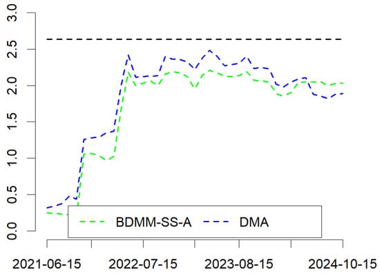
Figure 1.
Giacomini and Rossi fluctuation test. Horizontal black line represents critical value.
The estimated models were also constructed by replacing the dependent variable with the aluminum LME cash official closing prices (AH_C.F) values of the month (instead of monthly average) [23]. In such a case, the two top minimizing RMSE models were NAÏVE and ARIMA. Futures-based forecasts were third and fourth. Interestingly, the next most accurate models were BDMM-SS and BDMM-SS-A. In the case of MAE metric, NAÏVE and ARIMA were still the most accurate, but BDMM-SS was the third most accurate model. Similarly, considering MASE, ARIMA was most accurate, and BDMM-SS was second best. Details are presented in Table 5.
Table 5.
Forecast accuracy measures (forecasted monthly closing prices).
However, in the case of MASE, none of the models obtained an MASE less than 1. Unfortunately, Diebold–Mariano tests (not reported herein, but available upon request) suggest that competing methods are less accurate than NAÏVE, and BDMM-SS and DMA, at least in most cases, are not significantly more accurate than other non-trivial models. However, the MCS test did not eliminate any model (p-value 0.0688).
Another modification was to replace the exchange rates by the exchange rates of countries that are biggest producers of ore (bauxite), i.e., Australia (AUDUSD) and the Republic of Guinea (GNF) [23]. For GNF, monthly averages were taken from FXTOP [53]. In such a case, futures-based forecasts were still the most accurate according to all metrics. However, for the next most accurate models, these included BMS, BMA, DMS, and BMP, i.e., versions of the general DMA scheme [38,39]. Interestingly, in the case of MAE and MASE, it was LARS, EL-NET, LASSO, and RIDGE that were the most accurate. Still, the MCS test did not reject any model (p-value 0.0996). Detailed outcomes are not reported herein, due to the limited space.
4. Discussion
This study compared various aluminum price forecasting models, which are able to deal with variable selection problems and time-varying regression coefficients. In other words, they can deal with problems where the importance of price predictor changes over time, as well as its relationship strength with the predicted price changes. It was found that futures-based forecasts (in particular, end-of-month closing prices) can be a very accurate method when the monthly average aluminum price is predicted. Also, Dynamic Model Averaging is a promising forecasting scheme, whereas Bayesian dynamic mixture models performed less accurately than they were expected to. This adds some new value towards research into the usability of futures-based forecasts on commodity markets. However, in the case of predicting closing monthly prices, futures-based forecasts (also end-of-month closing prices) are still performing well, but Bayesian mixture models also become an interesting method, especially the state-space component version, as well as the one with an averaging scheme incorporated, outperforming Dynamic Model Averaging. On the other hand, for closing price forecasting, beating the no-change or ARIMA method is still a hard challenge. All of these results are in line with previous studies [2,54,55,56,57].
Author Contributions
Conceptualization, K.D.; methodology, K.D.; software, K.D.; validation, K.D. and J.J.; formal analysis, K.D.; investigation, K.D. and J.J.; resources, K.D.; data curation, K.D. and J.J.; writing—original draft preparation, K.D. and J.J.; writing—review and editing, K.D. and J.J.; visualization, K.D.; supervision, K.D.; project administration, K.D.; funding acquisition, K.D. All authors have read and agreed to the published version of the manuscript.
Funding
This research was funded in whole by National Science Centre, Poland, grant number 2022/45/B/HS4/00510.
Institutional Review Board Statement
Not applicable.
Informed Consent Statement
Not applicable.
Data Availability Statement
Republishing the full data is unavailable due to copyright restrictions. The majority of the data applied in the study are openly available as cited in the text (suitable tickers provided) and in the References. The forecast data generated in the study are openly available in RepOD at https://doi.org/10.18150/ERBJKK.
Acknowledgments
This research was funded in whole by National Science Centre, Poland, grant number 2022/45/B/HS4/00510. For the purpose of Open Access, the author has applied a CC-BY public copyright licence to any Author Accepted Manuscript (AAM) version arising from this submission.
Conflicts of Interest
The authors declare no conflicts of interest. The funders had no role in the design of the study; in the collection, analyses, or interpretation of the data; in the writing of the manuscript; or in the decision to publish the results.
References
- Alquist, R.; Kilian, L. What do we learn from the price of crude oil futures? J. Appl. Econom. 2010, 25, 539–573. [Google Scholar] [CrossRef]
- Buncic, D.; Moretto, C. Forecasting copper prices with dynamic averaging and selection models. N. Am. J. Econ. Financ. 2015, 33, 1–38. [Google Scholar] [CrossRef]
- Reynolds, D.B.; Umekwe, M.P. Shale-oil development prospects: The role of shale-gas in developing shale-oil. Energies 2019, 12, 3331. [Google Scholar] [CrossRef]
- Kahraman, E.; Akay, O. Comparison of exponential smoothing methods in forecasting global prices of main metals. Miner. Econ. 2023, 36, 427–435. [Google Scholar] [CrossRef]
- Kwas, M.; Paccagnini, A.; Rubaszek, M. Common factors and the dynamics of industrial metal prices: A forecasting perspective. Resour. Policy 2021, 74, 102319. [Google Scholar] [CrossRef]
- Liu, Q.; Liu, M.; Zhou, H.; Yan, F. A multi-model fusion based non-ferrous metal price forecasting. Resour. Policy 2022, 77, 102714. [Google Scholar] [CrossRef]
- Alquist, R.; Kilian, L.; Vigfusson, R.J. Forecasting the price of oil. In Handbook of Economic Forecasting; Elliott, G., Timmermann, A., Eds.; Elsevier: Amsterdam, Netherlands, 2013; Volume 2, Part A, pp. 427–507. [Google Scholar] [CrossRef]
- Gargano, A.; Timmermann, A. Forecasting commodity price indexes using macroeconomic and financial predictors. Int. J. Forecast. 2014, 30, 825–843. [Google Scholar] [CrossRef]
- He, Z.; Huang, J. A novel non-ferrous metal price hybrid forecasting model based on data preprocessing and error correction. Resour. Policy 2023, 86, 104189. [Google Scholar] [CrossRef]
- Ma, F.; Wahab, M.I.; Huang, D.; Xu, W. Forecasting the realized volatility of the oil futures market: A regime switching approach. Energy Econ. 2017, 67, 136–145. [Google Scholar] [CrossRef]
- Nguyen, D.K.; Walther, T. Modeling and forecasting commodity market volatility with long-term economic and financial variables. J. Forecast. 2020, 39, 126–142. [Google Scholar] [CrossRef]
- Pincheira, P.; Hardy, N. Forecasting aluminum prices with commodity currencies. Resour. Policy 2021, 73, 102066. [Google Scholar] [CrossRef]
- Croushore, D. Frontiers of real-time data analysis. J. Econ. Lit. 2011, 49, 72–100. [Google Scholar] [CrossRef]
- Nagy, I.; Suzdaleva, E. Mixture estimation with state-space components and Markov model of switching. Appl. Math. Model. 2013, 37, 9970–9984. [Google Scholar] [CrossRef]
- Nagy, I.; Suzdaleva, E.; Karny, M.; Mlynarova, T. Bayesian estimation of dynamic finite mixtures. Int. J. Adapt. Control Signal Process. 2011, 25, 765–787. [Google Scholar] [CrossRef]
- World Bank. Commodity Markets. 2025. Available online: https://www.worldbank.org/en/research/commodity-markets (accessed on 3 February 2025).
- Menzie, W.D.; Barry, J.J.; Bleiwas, D.I.; Bray, E.L.; Goonan, T.G.; Matos, G. The Global Flow of Aluminum from 2006 Through 2025: Open-File Report 2010–1256; U.S. Geological Survey: Reston, VA, USA, 2010. Available online: https://pubs.usgs.gov/of/2010/1256 (accessed on 3 February 2025).
- OECD. OECD Data Explorer. 2025. Available online: https://data-explorer.oecd.org (accessed on 3 February 2025).
- Westmetall. Market Data. 2025. Available online: https://www.westmetall.com/en/markdaten.php (accessed on 3 February 2025).
- International Aluminium Institute. Statistics. 2025. Available online: https://international-aluminium.org (accessed on 3 February 2025).
- ALFRED. Archival FRED. 2025. Available online: https://alfred.stlouisfed.org (accessed on 3 February 2025).
- FRED. Economic Data. 2025. Available online: https://fred.stlouisfed.org (accessed on 3 February 2025).
- Stooq. Stooq. 2025. Available online: https://stooq.pl/index.html (accessed on 3 February 2025).
- Kilian, L. Not all oil price shocks are alike: Disentangling demand and supply shocks in the crude oil market. Am. Econ. Rev. 2009, 99, 1053–1069. [Google Scholar] [CrossRef]
- Chicago Board Options Exchange. Historical Data. 2025. Available online: https://www.cboe.com/tradable_products/vix/vix_historical_data (accessed on 3 February 2025).
- Yahoo. Yahoo!finance. 2025. Available online: https://finance.yahoo.com (accessed on 3 February 2025).
- Shrivastava, P.; Vidhi, R. Pathway to sustainability in the mining industry: A case study of Alcoa and Rio Tinto. Resources 2020, 9, 70. [Google Scholar] [CrossRef]
- Barry, J.J.; Matos, G.R.; Menzie, W.D.U.S. Mineral Dependence—Statistical Compilation of U.S. and World Mineral Production, Consumption, and Trade, 1990–2010, Open-File Report 2013-1184; U.S. Geological Survey: Reston, VA, USA, 2013. Available online: https://pubs.usgs.gov/of/2013/1184 (accessed on 3 February 2025).
- Idoine, N.E.; Raycraft, E.R.; Hobbs, S.F.; Everett, P.; Evans, E.J.; Mills, A.J.; Currie, D.; Horn, S.; Shaw, R.A. World Mineral Production 2018–22; British Geological Survey: Keyworth, Nottingham, UK, 2024. Available online: https://nora.nerc.ac.uk/id/eprint/537241/1/World%20Mineral%20Production%202018%20to%202022.pdf (accessed on 3 February 2025).
- Koop, G.; Korobilis, D. Large time-varying parameter VARs. J. Econom. 2013, 177, 185–198. [Google Scholar] [CrossRef]
- Drachal, K. Determining time-varying drivers of spot oil price in a Dynamic Model Averaging framework. Energies 2018, 11, 1207. [Google Scholar] [CrossRef]
- Dickey, D.A.; Fuller, W.A. Distribution of the estimators for autoregressive time series with a unit root. J. Am. Stat. Assoc. 1979, 74, 427–431. [Google Scholar] [CrossRef]
- Phillips, P.C.B.; Perron, P. Testing for a unit root in time series regression. Biometrika 1988, 75, 335–346. [Google Scholar] [CrossRef]
- Kwiatkowski, D.; Phillips, P.C.B.; Schmidt, P.; Shin, Y. Testing the null hypothesis of stationarity against the alternative of a unit root. J. Econom. 1992, 54, 159–178. [Google Scholar] [CrossRef]
- Trapletti, A.; Hornik, K. Tseries: Time Series Analysis and Computational Finance. 2024. Available online: https://CRAN.R-project.org/package=tseries (accessed on 3 February 2025).
- Barbieri, M.M.; Berger, J.O. Optimal predictive model selection. Ann. Stat. 2004, 32, 870–897. [Google Scholar] [CrossRef]
- Drachal, K. “Dynmix”: An R package for the estimation of dynamic finite mixtures. SoftwareX 2023, 22, 101388. [Google Scholar] [CrossRef]
- Raftery, A.E.; Karny, M.; Ettler, P. Online prediction under model uncertainty via dynamic model averaging: Application to a cold rolling mill. Technometrics 2010, 52, 52–66. [Google Scholar] [CrossRef] [PubMed]
- Drachal, K. Dynamic Model Averaging in economics and finance with fDMA: A package for R. Signals 2020, 1, 47–99. [Google Scholar] [CrossRef]
- Friedman, J.; Hastie, T.; Tibshirani, R. Regularization paths for generalized linear models via coordinate descent. J. Stat. Softw. 2010, 33, 1–22. [Google Scholar] [CrossRef]
- Gramacy, R.B. Monomvn: Estimation for MVN and Student-t Data with Monotone Missingness. 2019. Available online: https://CRAN.R-project.org/package=monomvn (accessed on 3 February 2025).
- Hastie, T.; Efron, B. lars: Least Angle Regression, Lasso and Forward Stagewise. 2013. Available online: https://CRAN.R-project.org/package=lars (accessed on 3 February 2025).
- Hyndman, R.J.; Khandakar, Y. Automatic time series forecasting: The forecast package for R. J. Stat. Softw. 2008, 26, 1–22. [Google Scholar] [CrossRef]
- Ellwanger, R.; Snudden, S. Futures prices are useful predictors of the spot price of crude Oil. Energy J. 2023, 44, 65–82. [Google Scholar] [CrossRef]
- R Core Team. R: A Language and Environment for Statistical Computing; R Foundation for Statistical Computing: Vienna, Austria, 2018; Available online: https://www.R-project.org (accessed on 3 February 2025).
- Hyndman, R.J.; Koehler, A.B. Another look at measures of forecast accuracy. Int. J. Forecast. 2006, 22, 679–688. [Google Scholar] [CrossRef]
- Diebold, F.X.; Mariano, R.S. Comparing predictive accuracy. J. Bus. Econ. Stat. 1995, 13, 253–263. Available online: https://www.jstor.org/stable/1392155 (accessed on 3 February 2025). [CrossRef]
- Harvey, D.; Leybourne, S.; Newbold, P. Testing the equality of prediction mean squared errors. Int. J. Forecast. 1997, 13, 281–291. [Google Scholar] [CrossRef]
- Hansen, P.R.; Lunde, A.; Nason, J. The model confidence set. Econometrica 2011, 79, 453–497. [Google Scholar] [CrossRef]
- Bernardi, M.; Catania, L. The model confidence set package for R. Int. J. Comput. Econ. Econom. 2018, 8, 144–158. [Google Scholar] [CrossRef]
- Giacomini, R.; Rossi, B. Forecast comparisons in unstable environments. J. Appl. Econom. 2010, 25, 595–620. [Google Scholar] [CrossRef]
- Jordan, A.; Krueger, F. Murphydiagram: Murphy Diagrams for Forecast Comparisons. 2019. Available online: https://CRAN.R-project.org/package=murphydiagram (accessed on 3 February 2025).
- FXTOP. Historical Rates. 2025. Available online: https://fxtop.com/en/historical-exchange-rates.php (accessed on 3 February 2025).
- Drachal, K. Forecasting selected energy commodities prices with Bayesian dynamic finite mixtures. Energy Econ. 2021, 99, 105283. [Google Scholar] [CrossRef]
- Drachal, K. Forecasting prices of selected metals with Bayesian data-rich models. Resour. Policy 2019, 64, 101528. [Google Scholar] [CrossRef]
- Farag, M.; Snudden, S.; Upton, G. Can futures prices predict the real price of primary commodities? USAEE Work. Pap. 2024, 24, 629. [Google Scholar] [CrossRef]
- Kwas, M.; Rubaszek, M. Forecasting commodity prices: Looking for a benchmark. Forecasting 2021, 3, 447–459. [Google Scholar] [CrossRef]
Disclaimer/Publisher’s Note: The statements, opinions and data contained in all publications are solely those of the individual author(s) and contributor(s) and not of MDPI and/or the editor(s). MDPI and/or the editor(s) disclaim responsibility for any injury to people or property resulting from any ideas, methods, instructions or products referred to in the content. |
© 2025 by the authors. Licensee MDPI, Basel, Switzerland. This article is an open access article distributed under the terms and conditions of the Creative Commons Attribution (CC BY) license (https://creativecommons.org/licenses/by/4.0/).