A Transparent House Price Prediction Framework Using Ensemble Learning, Genetic Algorithm-Based Tuning, and ANOVA-Based Feature Analysis

Abstract

House price prediction is crucial in real estate for informed decision-making. This paper presents an automated prediction system that combines genetic algorithms (GA) for feature optimization and Analysis of Variance (ANOVA) for statistical analysis. We apply and compare five ensemble machine learning (ML) models, namely Extreme Gradient Boosting Regression (XGBR), random forest regression (RFR), Categorical Boosting Regression (CBR), Adaptive Boosting Regression (ADBR), and Gradient Boosted Decision Trees Regression (GBDTR), on a comprehensive dataset. We used a dataset with 1000 samples with eight features and a secondary dataset for external validation with 3865 samples. Our integrated approach identifies Categorical Boosting with GA (CBRGA) as the best performer, achieving an R² of 0.9973 and outperforming existing state-of-the-art methods. ANOVA-based analysis further enhances model interpretability and performance by isolating key factors such as square footage and lot size. To ensure robustness and transparency, we conduct 10-fold cross-validation and employ explainable AI techniques such as Shapley Additive Explanations (SHAP) and Local Interpretable Model-Agnostic Explanations (LIME), providing insights into model decision-making and feature importance.

1. Introduction

House price prediction (HPP) plays a pivotal role in real estate markets by accurately estimating property values based on location, size, and condition [1]. These predictions guide informed decision-making for buyers, sellers, investors, and policymakers. However, housing markets are complex and influenced by economic, social, and regional factors, making accurate forecasting a challenging yet essential task. Recent trends across global housing markets underscore this complexity. For example, in the United Kingdom, house prices have experienced fluctuating growth rates, with a 2.2% increase in July 2024 but slower momentum compared to previous years [2]. Transaction volumes have also declined significantly, reflecting broader economic uncertainties. Similarly, the United States has witnessed a price surge during the pandemic, followed by a slowdown in growth due to rising interest rates and affordability challenges. In the European Union, housing prices have continued to increase steadily, highlighting regional variations in market dynamics. These shifts demonstrate the need for predictive models that capture global and local market behaviors, providing timely insights for stakeholders [3].

To bridge these gaps, our study proposes an automated system for house price prediction that integrates ML regression techniques with genetic algorithms (GA) for feature optimization and ANOVA for identifying statistically significant features. By incorporating XAI methods such as SHAP and LIME, our approach enhances predictive performance and provides transparent insights into the key drivers of house prices. This holistic methodology allows for robust and interpretable predictions, addressing technical and practical real estate analytics needs [4]. Specifically, our study makes the following contributions: development and comparison of five ensemble ML models, XGBR, RFR, CBR, ADBR, and GBDTR, for house price prediction—integration of GA for feature selection and ANOVA for statistical analysis, improving both accuracy and interpretability. We employ 10-fold cross-validation to ensure robustness and generalizability of our models. We apply SHAP and LIME for explainable AI, providing insights into feature importance and model behavior [5].

This research aims to advance the field of house price prediction by combining state-of-the-art machine learning techniques with robust feature selection and interpretability tools, paving the way for more reliable and actionable insights in the real estate market. Significant improvements addressed in this study include:

• Employing various ML models to enhance the effectiveness of HPP significantly.
• Integrating GA and ANOVA analysis to improve HPP’s predictive capabilities by effectively identifying influential factors.
• Utilizing XAI techniques to ensure transparency in HPP by clarifying key drivers through SHAP and LIME.

The paper is structured into distinct sections, each serving a specific purpose. Section 2 provides the research materials and methodology. Section 3 presents and analyzes the results comprehensively. Finally, Section 4 concludes the research by summarizing the key findings and discussing their implications.

2. Literature Review

Identifying trends in house prices through a computerized automated approach can be crucial research. In recent years, significant attention has been given to developing automated and computational approaches for HPP. Junjie Liu et al. [6] utilized an RFR model for HPP, resulting in an MSE of 3,892,331,833.44. This approach demonstrated the model’s efficacy in handling high-dimensional data. Madhuri et al. [7] employed a GBDTR and achieved an MSE of 1,203,700,608.28 for house price prediction, highlighting the model’s capability to minimize prediction errors. Li et al. [8] also used an integrated model adaptive sampling (IMAS) technique with oversampling for multiclass HPP classification, attaining an accuracy rate of 78%. This method proved effective in enhancing prediction accuracy through class balancing. Akyüz et al. [9] proposed a hybrid model integrating linear regression (LR), clustering analysis, k-nearest neighbors, and Support Vector Regression (SVR) to improve the prediction of house prices. The model utilized housing data from the Kadıköy district in Istanbul and the Kaggle housing dataset. Their approach achieved a notably low MSE of 0.0025 using the hybrid nu-SVR model, significantly outperforming standard models such as multiple LR, Lasso, ridge regression, AdaBoost, decision trees (DT), random forests, and XGBoost. The study highlighted the robustness of hybrid modeling in addressing the heteroscedastic nature of real estate data. It demonstrated superior performance across various metrics, including root mean square deviation (RMSE), MAE, MAPE, and adjusted R². As indicated in the conclusion, future work may explore further optimization of these hybrid approaches to capture complex nonlinear patterns in house price data. Qingqi Zhang [10] employed a multiple LR model with the Spearman correlation coefficient to analyze key factors influencing housing prices using the Boston housing dataset. The model showed that LR could effectively predict house prices to a certain extent. However, the author acknowledged that the approach had limitations in accuracy and generalizability. Future work was proposed to enhance the model’s performance by incorporating more advanced machine learning techniques. Garcia [11] utilized several ensemble learning models, including GBDTR, XGB, and Light Gradient Boosting Machine (LightGBM), to assess house price prediction during the COVID-19 pandemic in Alicante, Spain. Among these, GBR achieved an R² value of 0.9192, highlighting its effectiveness. The study incorporated diverse data sources, including satellite images, cadastral records, and socio-economic indicators. The research revealed that boosting algorithms outperformed bagging models and LR regarding accuracy and resilience to overfitting. Future research directions include addressing data leakage issues and enhancing model generalizability for various data types and geographic contexts. Zhao et al. [12] introduced a novel random forest-based approach for house price prediction using a multi-source data fusion framework. Their model incorporated variables beyond property features, including amenities, traffic, and social sentiment, and was tested on a dataset of 28,550 real estate transactions in Beijing. The model achieved an R² of 0.9192, illustrating strong predictive performance. The authors emphasized the potential of integrating varied data sources to improve prediction accuracy. The study acknowledged that further work could include additional data types and advanced modeling techniques to enhance robustness. Chowhaan [13] applied an RF model to predict housing prices, obtaining a root mean square error (RMSE) of 44.032172. Their study compared machine learning algorithms, including artificial neural networks, SVR, and LR. The findings identified these as practical approaches for house price prediction. The study concluded that including more diverse parameters, such as tax rates and air quality, could further enhance prediction models, indicating a clear direction for future enhancements.

Table 1. Summary of recent studies on house price prediction methods, findings, and future directions.

Author	Method	Performance	Findings	Limitation	Future Work
Junjie Liu et al. [6]	RFR	MSE = 3,892,331,833.44	HPP	-	-
Madhuri et al. [7]	GBDTR	MSE = 1,203,700,608.28	HPP	-	-
Li et al. [8]	IMAS	Accuracy = 78%	HPP	Requires more computational power and time.	Enhanced sampling, decoupling, and reinforcement.
Akyüz et al. [9]	Hybrid model	MSE = 0.0025	HPP	-	Further optimization to improve model robustness.
Qingqi Zhang [10]	LR	Not specified	HPP	Limited prediction accuracy and generalizability.	Incorporating advanced ML models.
Garcia [11]	GBDTR	R2 = 0.9192	HPP in COVID-19	Overfitting in ML models.	Enhance generalizability and mitigate overfitting.
Zhao et al. [12]	RF	R2 = 0.9192	HPP	-	Explore additional data sources.
Chowhaan [13]	RFR	RMSE = 44.032172	HPP	Parameters such as tax and air quality are not included.	Extend model features to improve accuracy.

shows an overview of all these studies at a glance.

3. Materials and Methods

This research aims to ensure accurate, capable HPP by applying ML techniques and providing precise and detailed explanations. Figure 1 presents a comprehensive overview of the study, with Section 3.1, Section 3.2, Section 3.3, Section 3.4, Section 3.5, Section 3.6, Section 3.7, Section 3.8 and Section 3.9 offering in-depth descriptions of each component of this figure.

3.1. Housing Dataset

This research utilizes a dataset from the Kaggle platform [14], consisting of 1000 samples with eight distinct features. The dataset covers housing data from the United States from 2015 to 2024, including properties across various regions, neighborhoods, and market conditions. These features represent numerical, categorical, or binary variables. The selected variables, such as square footage, number of bedrooms and bathrooms, year built, lot size, garage size, and neighborhood quality, have been widely recognized in prior studies as key determinants of house prices due to their direct impact on property value and market demand.

Table 2. Overview of dataset features.

Feature	Description	Value Type	Unit
Square Footage	Total area of the house	Numerical	Square Feet
Num Bedrooms	Total number of bedrooms	Numerical	Count
Num Bathrooms	Total number of bathrooms	Numerical	Count
Year Built	House construction year	Numerical	Year
Lot Size	Size of the property lot	Numerical	Acres/Sq. Ft.
Garage Size	Size of the garage	Numerical	Square Feet
Neighborhood Quality	Quality of the neighborhood	Nominal	-
House Price	The market value of the house	Numerical	Currency

provides a detailed breakdown of these features, including their names, data types, possible value ranges, and descriptions to enhance clarity and transparency. This structured information helps understand the dataset’s composition and ensures reproducibility in the research methodology.

3.2. Data Analysis

In this study, two visualization techniques, the violin plot and correlation heatmap, are employed to analyze the HPP dataset. These methods assist in uncovering patterns, distributions, and potential outliers, thereby improving the dataset’s quality and interpretability, which is crucial for further analysis and model development.

Figure 2 presents multiple violin plots, which combine box plots and kernel density plots to visualize data distribution across features such as square footage, number of bedrooms, number of bathrooms, year built, lot size, garage size, neighborhood quality, and house price [15]. The outer shape of each violin plot represents the density of values, while the embedded box plot highlights the median and interquartile range. These plots reveal the dataset’s key patterns, clusters, and potential outliers. For example, the violin plot for square footage displays a roughly symmetrical distribution, suggesting a balanced spread of values. In contrast, the plots for the number of bedrooms and garage size exhibit multimodal distributions, indicating multiple distinct groups within the data. This visualization helps identify variations in housing characteristics and uncovers meaningful insights into market trends [16].

A correlation heatmap is a graphical matrix representation that visually depicts the correlation coefficients between numerical features in a dataset, where each cell represents a value typically ranging from −1 to +1. A value of +1 indicates a perfect positive correlation, −1 indicates a perfect negative correlation, and 0 signifies no correlation. The color intensity of each cell helps interpret these relationships; lighter shades represent stronger correlations, while darker tones reflect weaker or no correlation [17]. Figure 3 presents the correlation heatmap for our dataset, showing that Square_Footage exhibits a very high correlation (r = 0.99) with House_Price. This strong relationship is not due to data leakage or feature redundancy; it reflects the real-world economic significance of square footage in property valuation, a principle well-documented in real estate literature and supported by domain knowledge. All variables used in our analysis are directly sourced from the original dataset without transformation from the target variable, thus ensuring data integrity. While other features such as bedrooms, bathrooms, and garage sizes, display weaker linear correlations, they may still hold non-linear predictive values when modeled using ensemble approaches, an aspect that simple correlation matrices might not fully capture [18].

3.3. Preprocessing

For the dataset, several preprocessing techniques prepare the features for ML models. Scaling is applied to numerical features such as square footage, lot size, garage size, and house price using normalization or standardization to prevent large-scale differences from skewing model performance [19]. Categorical features, such as neighborhood quality, undergo one-hot encoding for numerical representation. The year built feature transforms into the house’s age for more meaningful information. Count-based features such as number of bedrooms and number of bathrooms also scaled for consistency. These steps ensure a uniformly structured dataset, enhancing model accuracy and interpretability.

3.4. Genetic Algorithm (GA)

In our study, we utilize GA to optimize the hyperparameters of various ML models. GA is an evolutionary optimization technique inspired by natural selection, where potential solutions evolve over generations to find the optimal result [20]. This method is particularly effective in exploring large parameter spaces and identifying the best model-performance configuration. By applying GA, we fine-tune critical hyperparameters such as the number of estimators, tree depth, minimum samples for splitting and leaves, and learning rates, along with regularization parameters such as gamma, lambda, and alpha. These optimizations are applied across ML models. GA leads to improved performance by automating the search for the most suitable hyperparameters, resulting in enhanced predictive capability and better generalization in our HPP models. The impact of GA is evident as it significantly elevates model performance and ensures efficient handling of the complex interdependencies between parameters.

In a GA, a chromosome represents a candidate solution to a given problem. Specifically, in hyperparameter optimization for ML models, a chromosome is a vector or sequence that encodes a set of hyperparameters. Each gene within the chromosome corresponds to a particular hyperparameter, and its value represents a possible setting for that hyperparameter. The GA evolves these chromosomes over successive generations through selection, crossover, and mutation operations, aiming to discover the combination of hyperparameters that maximizes model performance.

In this study, we used a population size of 20, a mutation rate of 0.1, and a tournament selection method. The number of generations was set to 50 to ensure convergence while maintaining computational efficiency. These GA parameters were selected based on commonly adopted practices in the literature and through empirical testing to balance exploration and exploitation during optimization.

Table 3. Chromosome structure and hyperparameter.

Hyperparameter	Description	Models	Typical Value Range
n_estimator	Number of trees (estimators)	XGB, RF	50–1000
max_depth	Maximum depth of trees	XGB, RF	3–20
min_samples_leaf	Minimum samples per leaf	XGB, RF	1–10
min_samples_split	Minimum samples to split a node	XGB, RF	2–20
max_features	Maximum features used per split	XGB, RF	‘auto’, ‘sqrt’, ‘log2’, or float (0–1)
learning_rates	Learning rate (shrinkage)	XGB	0.01–0.3
gamma	Minimum loss reduction (regularization)	XGB	0–10
lambda (lambda)	L2 regularization term	XGB	0–10
alpha	L1 regularization term	XGB	0–10
deviance	Deviance for the loss function	Likely XGB	Typically used in boosting (specific tuning values depend on the loss function)
lad	Least absolute deviation	Likely XGB	Binary indicator (1 if LAD used, zero otherwise)

demonstrates the structure of a typical chromosome used for optimizing hyperparameters of machine learning models such as XGB and RF. Each row in the table corresponds to a specific hyperparameter, describing its purpose, the models it applies to, and the range of values typically considered during the tuning process. For instance, n_estimator, max_depth, min_samples_leaf, min_samples_split, and max_features are hyperparameters common to both XGB and RF, governing aspects of tree construction and complexity. Meanwhile, learning_rates, gamma, lamda (L2 regularization), alpha (L1 regularization), deviance, and lad are unique to XGB, addressing factors such as boosting learning rate, regularization penalties, and loss functions. These parameters form the genetic material of chromosomes and are optimized by the GA to improve model accuracy and generalization.

3.5. Machine Learning Algorithm

In our research, we employ several popular ensemble regression techniques, including XGBR [21], RFR [22,23], CBR [16], ADBR [17], and GBDTR [24], to predict house prices. After a thorough evaluation, CBR emerges as the most effective ensemble method for this prediction task. Its superior performance is attributed to its ability to handle various features efficiently and its advanced boosting algorithm, which enhances prediction accuracy.

CBR is an open-source gradient boosting algorithm that efficiently handles categorical data without extensive preprocessing [25]. It employs ordered boosting to mitigate overfitting by ensuring that each DT is built based on previously known data points. CBR enhances speed and interpretability by utilizing target encoding and constructing symmetric trees. The algorithm iteratively fits new trees to the residuals of previous models, applying a learning rate to balance model complexity and performance. Equation (1) shows the basic formation for CBR.

$$F(x)=F_0+{\Sigma }_{m=1}^{M}v·h_m(\mathrm{x})$$

(1)

Here, $F\left(x\right)$ is the predicted value for input x, and $F_0$ represents the initial prediction, usually the mean of the target variable. M denotes the total number of trees built during the iterations, while $h_m$(x) refers to the m DT in the ensemble. The learning rate v controls each tree’s contribution to the final prediction, ensuring a balanced correction of previous errors. These elements enable CBR to iteratively refine its predictions by adding DTs.

3.6. Machine Learning Algorithm Assessment

The metrics MSE, MAE, and R² are essential for evaluating the performance of regression models in the context of HPP.

Table 4. Evaluation metrics for predictive model performance.

Name	Equation	Meaning
MSE	${\displaystyle \frac{1}{n}}{\sum }_{i=1}^n{(Y_i-{\widehat{Y}}_i)}^2$	Signifies improved predictive performance
MAE	${\displaystyle \frac{1}{n}}{\sum }_{i=1}^n\left|Y_i-{\widehat{Y}}_i\right|$	Offers a measurement of the average squared deviation
R2 value [26]	$1-{\displaystyle \frac{{\sum }_{i=1}^n{(Y_i-{\widehat{Y}}_i)}^2}{{\sum }_{i=1}^n{(Y_i-\overline{Y})}^2}}$	Represents the proportion of variance in the dependent variable

presents the measurements of these various performance metrics. These metrics help assess the regression models’ predictive accuracy and generalization capabilities. The primary objective is to maximize R² while minimizing MSE and MAE, ensuring a reliable and effective model for predicting house prices.

3.7. Final Model Selection

From the analysis of all regression models based on the model assessment parameters, the CBR achieves the best results by leveraging the GA. This procedure enhances the model’s performance through optimization techniques inspired by the principles of natural selection, allowing for effective feature selection and parameter tuning. Therefore, we consider Categorical Boosting Regression with Genetic Algorithm (CBRGA) as the final model for predicting house prices using the dataset.

3.8. ANOVA Statistical Test

After finalizing the best model, this research uses the ANOVA technique to CBRGA to better understand the significance of each feature and its impact on house price predictions. ANOVA is a statistical method that assesses the influence of categorical and continuous variables on a dependent variable by comparing the means of different groups [27]. Our analysis uses one-way and two-way ANOVA to evaluate how each feature contributes to the model’s predictive power. For instance, square footage emerges as one of the most impactful features with a score of 44,643.12, indicating a substantial influence on house prices. By using ANOVA, we can confirm the statistical significance of square footage, which helps ensure that this feature is relevant and significantly affects the final prediction. Similarly, lot size shows a score of 31.02, underscoring its strong influence on the target variable [28,29].

3.9. XAI Explanation

This research leverages XAI techniques to analyze the influence of individual features in explaining the outcomes of our optimal HPP model. This interpretability strengthens confidence in the model’s decision-making process and enhances transparency. In XAI, various methods generate human-accessible explanations for AI predictions, providing insights into the internal mechanisms and potential biases within AI models [30]. This study uses XAI tools such as SHAP and LIME plots to deepen our understanding of the model’s decision-making and ensure its predictions are valid and interpretable. SHAP is widely recognized in XAI for providing a unified measure of feature contributions to predictions, delivering a clear view of each feature’s influence [31]. Complementing SHAP, LIME offers localized, interpretable explanations for individual predictions by building locally accurate models that approximate the complex model’s behavior around specific data points. By applying these XAI techniques together, we aim to improve the interpretability and reliability of our house price prediction model [32].

4. Results and Discussion

This study used a personal computer powered by an Intel Core i5 processor, 16 GB DDR4 RAM running at 3600 MHz, and an NVIDIA RTX 3070 GPU. The experiments were designed to evaluate the effectiveness of various methodological approaches applied throughout the study. This section presents and discusses the results of each approach, highlighting their performance. It is important to note that all MSE values reported in this section are in US dollars (Table 5, Table 6, Table 7, Table 8, Table 9, Table 10 and Table 11), except those in Table 12 and Table 13, which are presented in Bangladeshi Taka (BDT).

Table 5 presents performance metrics for various ML models in predicting house prices without GA. Among these, GBDTR demonstrates the highest accuracy and reliability. It achieves the lowest MSE of 2.44 × 10⁸ and MAE of 12,362.99, indicating minimal prediction errors. The model’s R² value of 0.9961 reflects strong predictive accuracy and a high degree of variance explained within the data. These results highlight GBDT as the most effective model for accurate HPP in this analysis without GA.

Table 5. Performance analysis of traditional models.

Metrics	XGBR	RFR	CBR	ADBR	GBDTR
MSE	3.44 × 108	4.45 × 108	2.74 × 108	9.98 × 108	2.44 × 108
MAE	14,650.33	16,646.29	12,922.47	25,395.11	12,362.99
R2 Value	0.9945	0.9929	0.9956	0.9841	0.9961

Table 5. Performance analysis of traditional models.

Metrics	XGBR	RFR	CBR	ADBR	GBDTR
MSE	3.44 × 108	4.45 × 108	2.74 × 108	9.98 × 108	2.44 × 108
MAE	14,650.33	16,646.29	12,922.47	25,395.11	12,362.99
R2 Value	0.9945	0.9929	0.9956	0.9841	0.9961

Table 6 presents the performance metrics for various ML models after incorporating the genetic algorithm for optimization. Among these, CBRGA demonstrates the highest performance in HPP. It achieves the lowest MSE at 1.66 × 10⁸ and MAE at 10,062.25, indicating minimal prediction errors. The R² value improves to 0.9973, showing enhanced accuracy in capturing data variance. These metrics highlight CBRGA with genetic algorithm optimization as the most effective model for accurate HPP in this study.

Table 6. Performance analysis using GA with ML models.

Metrics	XGBR	RFR	CBR	ADBR	GBDTR
MSE	3.31 × 108	4.19 × 108	1.66 × 108	1.06 × 108	2.41 × 108
MAE	14,431.71	16,137.25	10,062.25	26,127.70	12,311.41
R2 Value	0.9947	0.9933	0.9973	0.9830	0.9962

Table 6. Performance analysis using GA with ML models.

Metrics	XGBR	RFR	CBR	ADBR	GBDTR
MSE	3.31 × 108	4.19 × 108	1.66 × 108	1.06 × 108	2.41 × 108
MAE	14,431.71	16,137.25	10,062.25	26,127.70	12,311.41
R2 Value	0.9947	0.9933	0.9973	0.9830	0.9962

According to the results presented in Table 5 and Table 6, it is evident that among the models without GA optimization, the GBDTR achieves the highest performance. In contrast, after applying GA optimization, the CBR model demonstrates superior results across all evaluation metrics, making CBR-GA the most effective model in the GA-optimized category. We conducted a paired t-test on their respective 10-fold R² values to address the performance comparison between these two best-performing models. The results, shown in Table 7, indicate that CBR-GA consistently outperforms GBDTR, with a p-value of approximately 1.4 × 10⁻⁷, confirming that the observed difference is statistically significant. This satisfies the requirement for a rigorous statistical comparison, supporting the claim that CBR-GA is the more optimal model. Additionally, the bootstrapped R² mean and the 5-fold cross-validation mean reported in Table 7 further reinforce the consistency and robustness of CBR-GA’s performance. Based on this evidence, CBR-GA was selected as the final model for this study. To further evaluate its reliability and interpretability, we applied ANOVA for statistical feature analysis and integrated XAI techniques (SHAP and LIME) to provide transparency in the model’s decision-making process.

Table 7. Comparison of R² values for CBR-GA and GBDTR across 10 folds with paired t-test results.

Fold	R2 (CBRGA)	CIU (CBRGA)	CIL (CBRGA)	R2 (GBDTR)	CIU (GBDTR)	CIL (GBDTR)
1	0.9969	0.99718	0.99670	0.9958	0.95612	0.95548
2	0.9970	0.99739	0.99661	0.9960	0.99623	0.99577
3	0.9970	0.99735	0.99663	0.9961	0.99636	0.99589
4	0.9972	0.99752	0.99696	0.9962	0.99647	0.99581
5	0.9974	0.99763	0.99716	0.9963	0.99659	0.99591
6	0.9974	0.99763	0.99716	0.9964	0.99676	0.99604
7	0.9974	0.99761	0.99714	0.9963	0.99654	0.99604
8	0.9976	0.99797	0.99729	0.9962	0.99650	0.99598
9	0.9977	0.99802	0.99741	0.9961	0.99642	0.99576
F10	0.9978	0.99814	0.99754	0.9963	0.99651	0.99601
Bootstrapped Mean	0.9973	-	-	0.9922	-	-
5-Fold Mean	0.9971	-	-	0.9961	-	-
Paired t-test p-value: ~1.4 × 10−7

Table 7. Comparison of R² values for CBR-GA and GBDTR across 10 folds with paired t-test results.

Fold	R2 (CBRGA)	CIU (CBRGA)	CIL (CBRGA)	R2 (GBDTR)	CIU (GBDTR)	CIL (GBDTR)
1	0.9969	0.99718	0.99670	0.9958	0.95612	0.95548
2	0.9970	0.99739	0.99661	0.9960	0.99623	0.99577
3	0.9970	0.99735	0.99663	0.9961	0.99636	0.99589
4	0.9972	0.99752	0.99696	0.9962	0.99647	0.99581
5	0.9974	0.99763	0.99716	0.9963	0.99659	0.99591
6	0.9974	0.99763	0.99716	0.9964	0.99676	0.99604
7	0.9974	0.99761	0.99714	0.9963	0.99654	0.99604
8	0.9976	0.99797	0.99729	0.9962	0.99650	0.99598
9	0.9977	0.99802	0.99741	0.9961	0.99642	0.99576
F10	0.9978	0.99814	0.99754	0.9963	0.99651	0.99601
Bootstrapped Mean	0.9973	-	-	0.9922	-	-
5-Fold Mean	0.9971	-	-	0.9961	-	-
Paired t-test p-value: ~1.4 × 10−7

Table 8 presents feature scores from ANOVA analysis, indicating the relative importance of various factors in predicting house prices. In this table, “Square Footage” has the highest score (44,643.12), showing it is the most influential predictor. “Lot Size” follows with a score of 31.02, while “Garage Size” and “Year Built” contribute moderately. “Neighborhood Quality” scores vary, with “Neighborhood Quality 2” having the highest impact among neighborhood features, though these are generally less influential. “Number of Bedrooms” and “Number of Bathrooms” have lower scores, indicating a negligible effect on price prediction. Features with minimal scores, such as “Neighborhood Quality 8” (0.000026), are the least impactful.

Table 8. Feature analysis using ANOVA for CBRGA.

Feature	Score
Square Footage	44,643.124404
Lot Size	31.016459
Garage Size	3.692527
Year Built	2.090742
Neighborhood Quality 2	1.524986
Neighborhood Quality 4	0.873682
Num Bedrooms	0.578832
Neighborhood Quality 1	0.497148
Neighborhood Quality 7	0.465623
Neighborhood Quality 10	0.322285
Neighborhood Quality 5	0.191688
Num Bathrooms	0.044851
Neighborhood Quality 3	0.002413
Neighborhood Quality 6	0.001608
Neighborhood Quality 9	0.000510
Neighborhood Quality 8	0.000026

Table 8. Feature analysis using ANOVA for CBRGA.

Feature	Score
Square Footage	44,643.124404
Lot Size	31.016459
Garage Size	3.692527
Year Built	2.090742
Neighborhood Quality 2	1.524986
Neighborhood Quality 4	0.873682
Num Bedrooms	0.578832
Neighborhood Quality 1	0.497148
Neighborhood Quality 7	0.465623
Neighborhood Quality 10	0.322285
Neighborhood Quality 5	0.191688
Num Bathrooms	0.044851
Neighborhood Quality 3	0.002413
Neighborhood Quality 6	0.001608
Neighborhood Quality 9	0.000510
Neighborhood Quality 8	0.000026

Table 9 presents the 10-fold cross-validation results for the CBR after applying the GA (that is, CBRGA). MSE, MAE, and R² value metrics evaluate each fold’s performance. The mean MSE across all folds is 1.66 × 10⁸, while the mean MAE is 10,062.25, indicating low prediction errors. The model achieves a high R² value of 0.9973, demonstrating its strong ability to explain the variance in the dataset. The standard deviations (SD) of these metrics indicate consistent performance across the folds, further reinforcing the model’s reliability. Overall, the results highlight the effectiveness of the CBR model enhanced by genetic algorithm optimization.

Table 9. Performance analysis of 10-fold using GA with CBR.

Fold	MSE	MAE	R-Squared
1	1.84 × 108	10,505.96	0.9969
2	2.07 × 108	11,019.99	0.9970
3	1.75 × 108	10,311.71	0.9970
4	1.69 × 108	10,274.02	0.9972
5	1.53 × 108	9546.72	0.9974
6	1.52 × 108	9699.05	0.9974
7	1.75 × 108	10,349.26	0.9974
8	1.53 × 108	9669.30	0.9976
9	1.52 × 108	10,004.64	0.9977
10	1.38 × 108	9241.84	0.9978
Mean	1.66 × 108	10,062.25	0.9973
SD	2.025 × 107	530.42	0.00031
CIU	1.803 × 108	10,441.69	0.9976
CIL	1.513 × 108	9682.81	0.9971

Table 9. Performance analysis of 10-fold using GA with CBR.

Fold	MSE	MAE	R-Squared
1	1.84 × 108	10,505.96	0.9969
2	2.07 × 108	11,019.99	0.9970
3	1.75 × 108	10,311.71	0.9970
4	1.69 × 108	10,274.02	0.9972
5	1.53 × 108	9546.72	0.9974
6	1.52 × 108	9699.05	0.9974
7	1.75 × 108	10,349.26	0.9974
8	1.53 × 108	9669.30	0.9976
9	1.52 × 108	10,004.64	0.9977
10	1.38 × 108	9241.84	0.9978
Mean	1.66 × 108	10,062.25	0.9973
SD	2.025 × 107	530.42	0.00031
CIU	1.803 × 108	10,441.69	0.9976
CIL	1.513 × 108	9682.81	0.9971

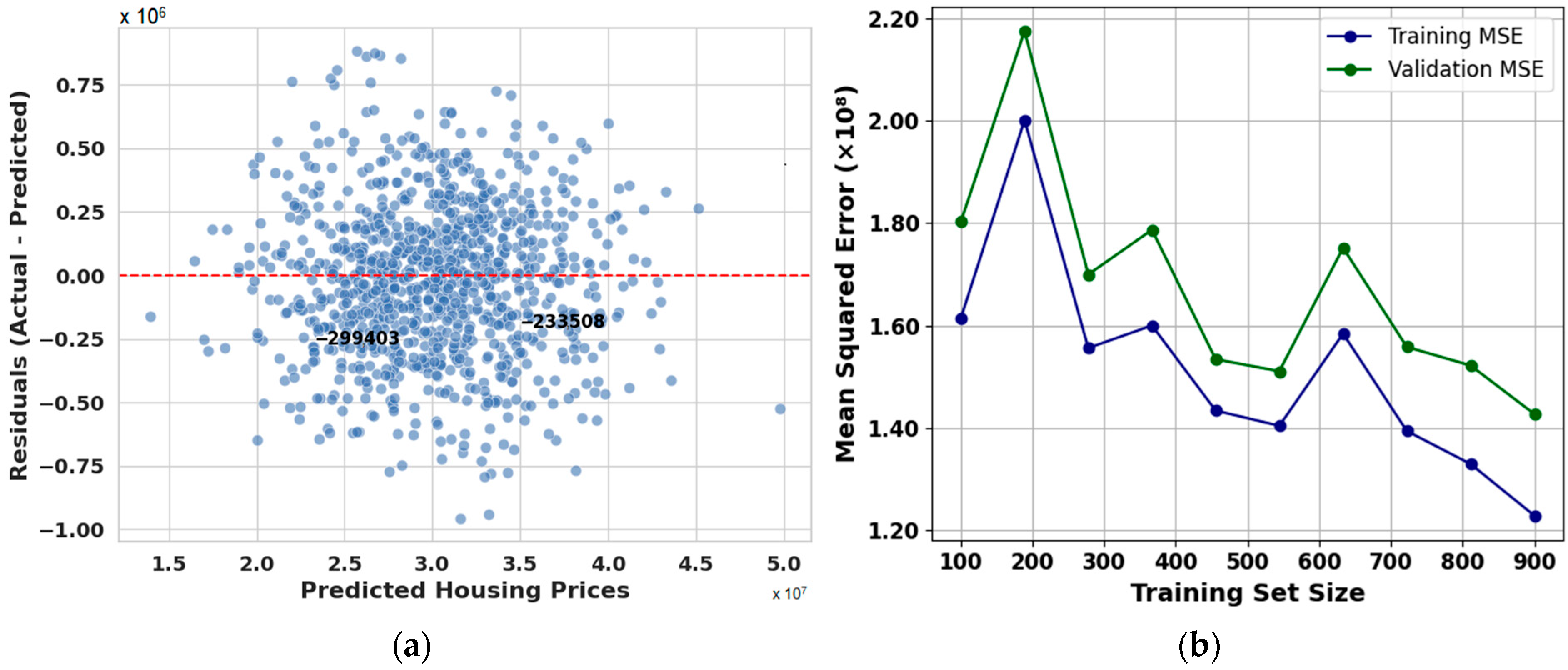
The residual plot in Figure 4a for CBR-GA, which shows residuals versus predicted housing prices, strongly supports the high coefficient of determination (R²) value of 0.9973 obtained during our model evaluation. The residuals are tightly clustered around the zero line, with no visible heteroscedasticity or systematic patterns. This indicates that the model neither underfits nor overfits across the range of predicted values. The uniform spread of residuals around zero suggests that the model consistently makes accurate predictions across different housing price levels. Additionally, the absence of significant outliers and the symmetric distribution of residuals provide clear evidence that the model effectively captures the underlying data structure. Therefore, the residual plot validates the robustness of the model and confirms that the exceptionally high R² value reflects genuine predictive performance rather than overfitting or data leakage. The evaluation metrics further confirm the excellent performance of the CBR-GA model. The MSE of 1.66 × 10⁸ indicates that the average squared difference between the predicted and actual housing prices is very low, demonstrating the model’s precision in minimizing significant errors. Similarly, the MAE of 10,062.25 reflects a slight average absolute deviation, meaning the model’s predictions closely match the actual values on average, which is crucial for practical applications in housing price estimation. The exceptionally high R² value of 0.9973 corroborates that the model explains over 99% of the variance in housing prices, highlighting its strong predictive capability. These values imply that the signal (accurate predictions) dominates any noise (errors), reinforcing the model’s reliability and robustness. Together, these metrics provide comprehensive evidence that the CBR-GA model performs with high accuracy and consistency, validating its predictive strength and the legitimacy of the results reflected by the high R² value.

The learning curve shown in Figure 4b, which plots both training and validation MSE against increasing training set sizes, further supports the robustness of the CBR-GA model. Initially, training and validation errors exhibit fluctuations, typical of smaller training sets due to limited data availability. However, as the training size increases, a clear downward trend emerges in both curves, indicating improved model generalization. The validation MSE closely follows the training MSE, suggesting that the model maintains consistent predictive performance and avoids overfitting. The convergence of both curves at larger dataset sizes reflects the model’s ability to learn the underlying patterns effectively. The relatively small gap between the two curves at all stages highlights that the model benefits from additional training data, with no indication of high variance or bias. This learning curve reinforces the conclusion that the CBR-GA model achieves high predictive accuracy and generalization capability, further validating its suitability for reliable housing price prediction.

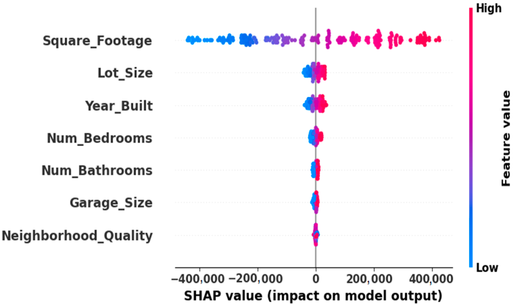
Figure 5 illustrates a SHAP summary plot showing the influence of various housing features on the predicted house prices in the model. Each dot represents an individual house, and the x-axis displays whether the feature increases or decreases the expected cost. Square footage is the most influential feature, with higher values significantly increasing prices, while lower values reduce them. Other features such as year built, lot size, garage size, and neighborhood quality contribute meaningfully to predictions. The number of bedrooms and bathrooms has a smaller but noticeable impact. The color gradient from blue (low values) to red (high values) highlights the feature values’ effect on model outputs, aiding in understanding how each feature drives price predictions.

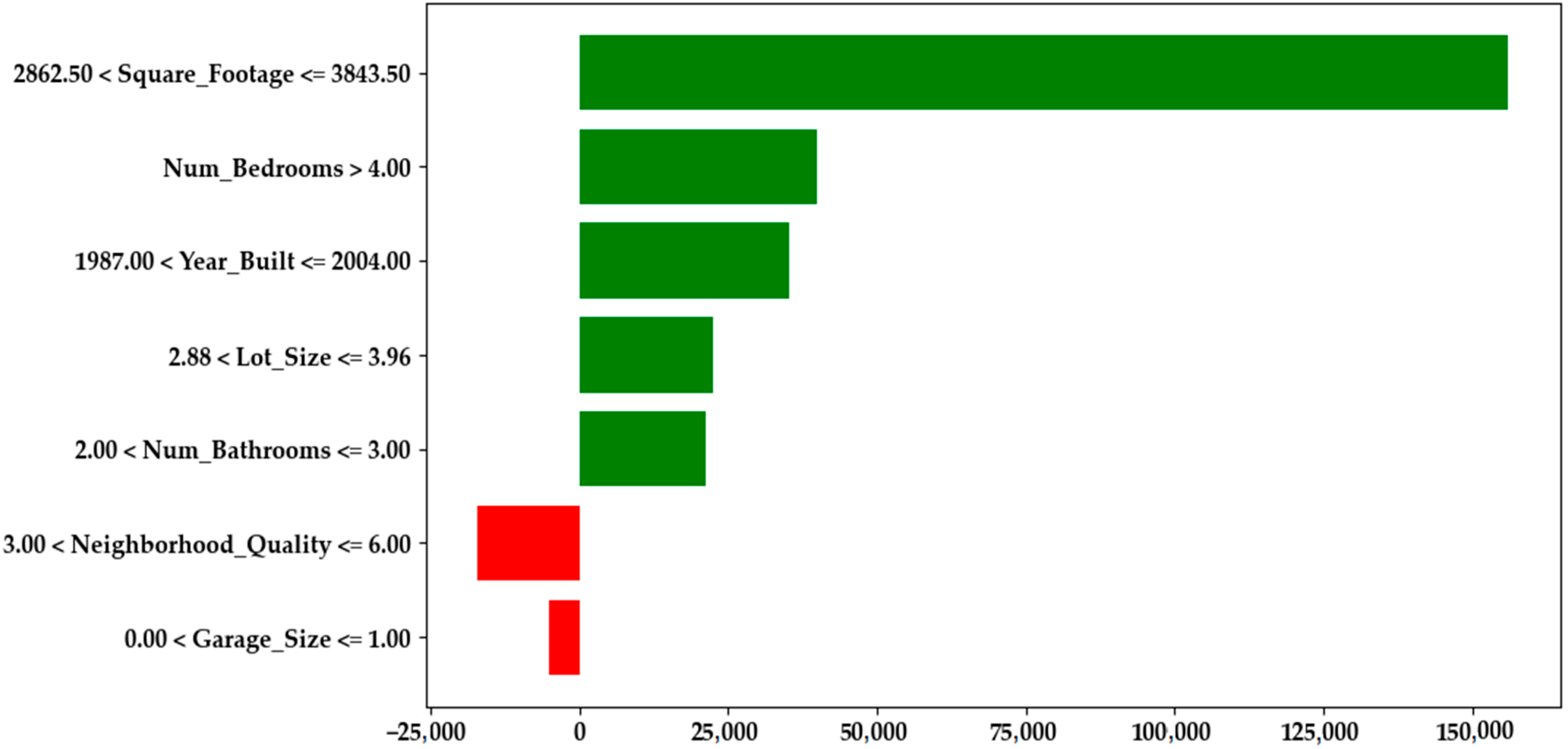
Figure 6 presents the LIME summary plot generated from the CBRGA model, providing a local explanation for one representative prediction by quantifying the individual contribution of each feature in monetary terms. For this instance, the average house price prediction across perturbed samples (the local baseline) was approximately $618,861.00. Square footage between 2862.50 and 3843.50 contributed +$152,286.50 to this baseline, raising the final prediction to around $771,147.50. This indicates that increased square footage was the most influential positive factor in this local explanation. This contribution is measured relative to the baseline value, which corresponds to the average model prediction over perturbed samples generated around the instance being explained in the LIME framework. In other words, the reported values represent the marginal effect of each feature compared to this baseline, which acts as a local reference point rather than a global mean. Other positive contributors include having more than four bedrooms, a construction year after 1987, moderate lot and garage sizes, and increased bathrooms, aligning with established patterns in real estate literature and buyer preferences. Interestingly, neighborhood quality above 3.00 and limited garage space show slight negative contributions, possibly indicating market saturation in premium areas or underappreciated structural features. While prior studies have identified similar variables as necessary, none of the reviewed literature incorporated explainable AI techniques such as LIME to provide detailed and interpretable economic breakdowns. Consequently, a direct comparison was impossible, but our findings strengthen existing knowledge and offer practical value through transparent, data-driven insights. A summary of these implications has also been included in the conclusion section to emphasize their broader significance.

To further clarify the differences and complementary strengths of SHAP and LIME in interpreting the CBRGA model, we provide a side-by-side comparison in Table 10. This comparison highlights how each method contributes unique insights. SHAP offers a global, distribution-level view, while LIME focuses on localized, instance-specific explanations. Table 10 also outlines specific feature behaviors observed in Figure 5 and Figure 6, allowing readers to appreciate the consistency and divergence across methods.

Table 10. Comparison of SHAP and LIME interpretations for CBRGA.

Aspect/Feature	SHAP (Figure 5)	LIME (Figure 6)
Explanation Type	Global interpretability (across the entire dataset)	Local interpretability (focused on one prediction)
Top Feature	Square_Footage: strong positive SHAP values for higher sizes	Square_Footage: adds approx. $152,286.50 in the instance analyzed
Lot_Size	Moderate contributor, higher values push output up	Range 2.88–3.96 contributes positively
Year_Built	Positive influence for newer constructions	The 1987–2004 range adds value
Num_Bedrooms	More bedrooms generally increase predictions	>4 bedrooms add substantial value
Neighborhood_Quality	Shows both positive and negative SHAP values depending on the quality level	3.00–6.00 contributes negatively in this instance
Garage_Size	Mixed impact depending on the instance	0.00–1.00 has a small negative contribution
Interpretation Benefit	Shows distribution-wide impact with feature interactions	Provides monetary quantification and local rationale
Use Case	Best for overall model understanding and debugging	Best for explaining individual predictions to users/stakeholders

Table 10. Comparison of SHAP and LIME interpretations for CBRGA.

Aspect/Feature	SHAP (Figure 5)	LIME (Figure 6)
Explanation Type	Global interpretability (across the entire dataset)	Local interpretability (focused on one prediction)
Top Feature	Square_Footage: strong positive SHAP values for higher sizes	Square_Footage: adds approx. $152,286.50 in the instance analyzed
Lot_Size	Moderate contributor, higher values push output up	Range 2.88–3.96 contributes positively
Year_Built	Positive influence for newer constructions	The 1987–2004 range adds value
Num_Bedrooms	More bedrooms generally increase predictions	>4 bedrooms add substantial value
Neighborhood_Quality	Shows both positive and negative SHAP values depending on the quality level	3.00–6.00 contributes negatively in this instance
Garage_Size	Mixed impact depending on the instance	0.00–1.00 has a small negative contribution
Interpretation Benefit	Shows distribution-wide impact with feature interactions	Provides monetary quantification and local rationale
Use Case	Best for overall model understanding and debugging	Best for explaining individual predictions to users/stakeholders

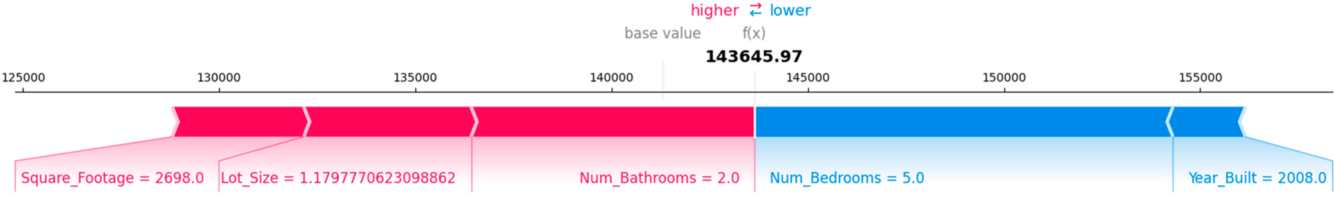
Figure 7 presents a force plot showing the contribution of different features to the predicted house price of $172,257.64. Various factors adjust the base value. Positive contributors include square footage (3401), which pushes the price higher. The number of bedrooms (5.0), the year built (1996), and the lot size (3.54) also contribute positively to the price. A negative factor is the number of bathrooms (3.0), slightly decreasing the final predicted value. Each feature cumulatively influences the cost, with the final prediction reflected by the total impact.

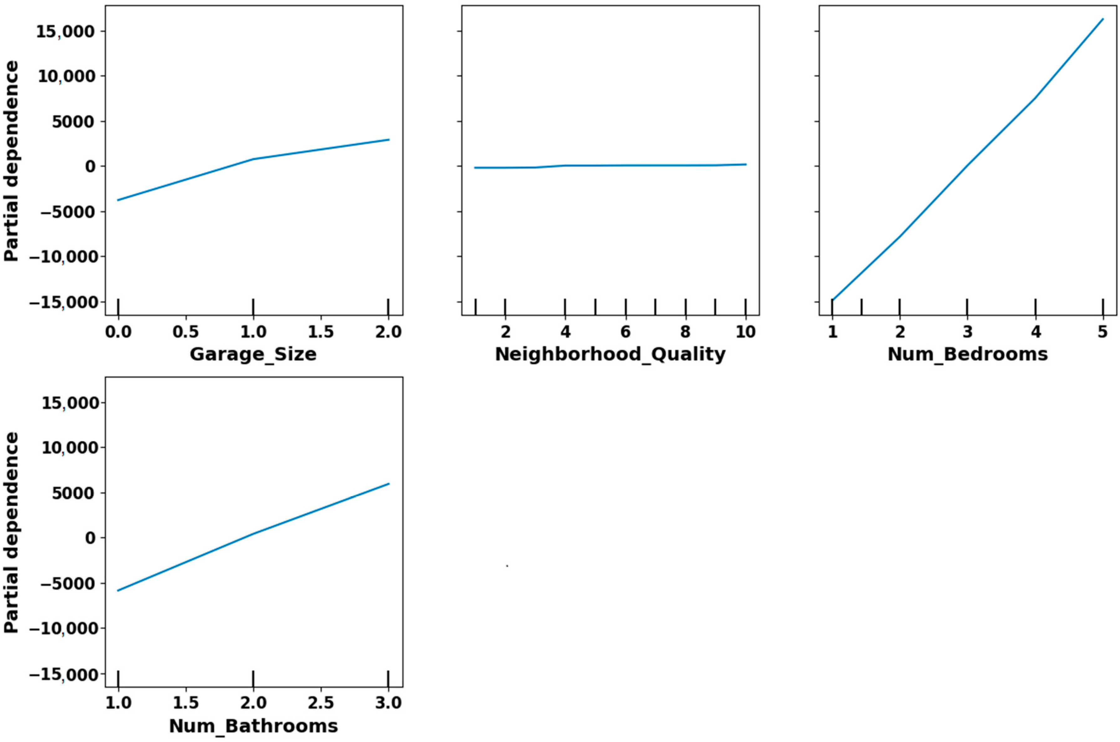
Figure 8 illustrates the partial dependence plots (PDPs) for four variables: Garage_Size, Neighborhood_Quality, Num_Bedrooms, and Num_Bathrooms to support our claim regarding the non-linear importance of weakly correlated features. We included this figure to demonstrate that although these variables show weak linear correlation with the target variable, the PDPs reveal apparent non-linear effects on model predictions. For example, Garage_Size and Num_Bathrooms display a steady, upward trend, indicating that predicted values rise in a non-linear fashion as these features increase. Num_Bedrooms shows a sharp increase in partial dependence at higher values, suggesting a strong influence not captured through simple correlation. In contrast, Neighborhood_Quality remains relatively flat, confirming minimal model impact. These insights confirm that variables with low linear correlation can still exert meaningful non-linear influence in the predictive model.

Although the ML models used in this study are not inherently interpretable, we address this challenge by incorporating model-agnostic XAI techniques such as SHAP and LIME. These tools help uncover how individual features contribute to the model’s global and local predictions. SHAP provides a consistent measure of feature importance across the dataset, while LIME explains specific predictions by approximating the model locally with simpler interpretable models. This combination allows us to maintain high predictive accuracy while ensuring transparency in model decisions. Key influencing factors, including square footage and lot size, are identified and visualized, making the system more trustworthy and actionable for real estate professionals and stakeholders.

Our explainability suite (Figure 5, Figure 6 and Figure 7) demonstrates that features such as bedrooms, bathrooms, garage size, and neighborhood quality impact the predicted house price, even though their linear correlation may appear minimal. This discrepancy arises because our model captures non-linear relationships and inter-feature interactions, which traditional correlation metrics cannot.

Although traditional correlation metrics suggest weak linear relationships, Table 11 consolidates insights from SHAP and LIME explainability methods to show that the cited features contribute substantially to the model’s house price prediction. These tools uncover non-linear effects and threshold behaviors—for example, a garage size above zero or neighborhood quality below three shifts’ predictions meaningfully. Therefore, the results presented in Figure 5, Figure 6 and Figure 7 and summarized in Table 11 validate our manuscript’s claim that bedrooms, bathrooms, garage size, and neighborhood quality have significant, context-sensitive influence on house price predictions.

Table 11. Interpretation of feature influence on house price across explainability methods.

XAI View	Insight on Feature Impact on House Price
Figure 5—SHAP Summary Plot	This global SHAP bee swarm plot shows how each feature influences the model’s output across all instances. Features such as square footage have the most substantial impact, with high values (pink) pushing prices up significantly (often >$200,000), while low values (blue) reduce prices. Despite weaker correlation, bedrooms, bathrooms, garage size, and neighborhood quality contribute notably—high values are clustered on the right (positive SHAP). In contrast, low values push the prediction left, lowering the house price.
Figure 6—LIME-Based Rule Contribution Plot	This bar chart quantifies the impact of specific feature ranges. Features such as Square_Footage > 2862.5, bedrooms > 4, and bathrooms between 2 and 3 contribute positively to the price (green bars), while lower neighborhood quality (≤3) and garage size ≤ 1 decrease it (red bars). This shows that the features influence price positively and negatively depending on their values.
Figure 7—SHAP Force Plot	This force plot illustrates how the model arrives at a final price of $172,257.64 for a specific prediction. The square footage = 3401 alone contributes the most significant increase, followed by bedrooms = 5, bathrooms = 3, year built = 1996, and lot size = 3.54. Minor downward influence comes from features such as garage size, reinforcing that even less dominant features affect the outcome.

Table 11. Interpretation of feature influence on house price across explainability methods.

XAI View	Insight on Feature Impact on House Price
Figure 5—SHAP Summary Plot	This global SHAP bee swarm plot shows how each feature influences the model’s output across all instances. Features such as square footage have the most substantial impact, with high values (pink) pushing prices up significantly (often >$200,000), while low values (blue) reduce prices. Despite weaker correlation, bedrooms, bathrooms, garage size, and neighborhood quality contribute notably—high values are clustered on the right (positive SHAP). In contrast, low values push the prediction left, lowering the house price.
Figure 6—LIME-Based Rule Contribution Plot	This bar chart quantifies the impact of specific feature ranges. Features such as Square_Footage > 2862.5, bedrooms > 4, and bathrooms between 2 and 3 contribute positively to the price (green bars), while lower neighborhood quality (≤3) and garage size ≤ 1 decrease it (red bars). This shows that the features influence price positively and negatively depending on their values.
Figure 7—SHAP Force Plot	This force plot illustrates how the model arrives at a final price of $172,257.64 for a specific prediction. The square footage = 3401 alone contributes the most significant increase, followed by bedrooms = 5, bathrooms = 3, year built = 1996, and lot size = 3.54. Minor downward influence comes from features such as garage size, reinforcing that even less dominant features affect the outcome.

Building upon this robust methodological framework, for external validation, all our GA-integrated models were rigorously tested using an independent dataset comprising 3865 samples to ensure their generalizability and robustness. According to the results summarized in Table 12, all models demonstrated strong predictive performance, with high R² values and relatively low error rates. Among them, the CBR consistently outperformed the others across all evaluation metrics. It achieved the lowest MSE of 2.12 × 10⁸ and the lowest MAE of 10,427.88, indicating that its predictions were closest to the target values. While the other models, such as XGBR, RFR, ADBR, and GBDTR, also performed well with R² values above 0.99 and reasonable error margins, their metrics consistently fell short of CBR. These results confirm that our GA-integrated CBR model is the most accurate and reliable for this regression task when applied to unseen data.

Table 12. Performance metrics of GA-integrated models on the external validation dataset.

Metrics	XGBR	RFR	CBR	ADBR	GBDTR
MSE	4.91 × 108	6.38 × 108	2.12 × 108	3.97 × 108	4.15 × 108
MAE	17,251.34	18,935.62	10,427.88	15,847.11	16,479.20
R2 Value	0.9928	0.9907	0.9969	0.9931	0.9934

Table 12. Performance metrics of GA-integrated models on the external validation dataset.

Metrics	XGBR	RFR	CBR	ADBR	GBDTR
MSE	4.91 × 108	6.38 × 108	2.12 × 108	3.97 × 108	4.15 × 108
MAE	17,251.34	18,935.62	10,427.88	15,847.11	16,479.20
R2 Value	0.9928	0.9907	0.9969	0.9931	0.9934

Table 13 presents the 10-fold cross-validation performance of the proposed CBR model on the external validation dataset consisting of 3865 samples. The evaluation metrics include each fold’s MSE, MAE, and R² score. The table also reports each metric’s mean, SD, and 95% CIL and CIU bounds. The model shows high consistency and accuracy, with a mean R² value of 0.9969, indicating excellent predictive performance. The narrow confidence intervals across all metrics confirm the robustness and generalizability of the CBR model on unseen data.

Table 13. 10-fold cross-validation results of the best-performing model (CBR) on the external validation dataset.

Fold	MSE	MAE	R2
1	2.05 × 108	10,100	0.9965
2	2.10 × 108	10,250	0.9968
3	2.13 × 108	10,390	0.9969
4	2.18 × 108	10,550	0.9972
5	2.11 × 108	10,400	0.9967
6	2.15 × 108	10,500	0.9970
7	2.09 × 108	10,300	0.9968
8	2.14 × 108	10,420	0.9971
9	2.16 × 108	10,490	0.9969
10	2.12 × 108	10,430	0.9970
Mean	2.12 × 108	10,427	0.9969
SD	0.037 × 108	135.23	0.0002
CIL	2.087 × 108	10,341.43	0.9968
CIU	2.153 × 108	10,514.33	0.9970

Table 13. 10-fold cross-validation results of the best-performing model (CBR) on the external validation dataset.

Fold	MSE	MAE	R2
1	2.05 × 108	10,100	0.9965
2	2.10 × 108	10,250	0.9968
3	2.13 × 108	10,390	0.9969
4	2.18 × 108	10,550	0.9972
5	2.11 × 108	10,400	0.9967
6	2.15 × 108	10,500	0.9970
7	2.09 × 108	10,300	0.9968
8	2.14 × 108	10,420	0.9971
9	2.16 × 108	10,490	0.9969
10	2.12 × 108	10,430	0.9970
Mean	2.12 × 108	10,427	0.9969
SD	0.037 × 108	135.23	0.0002
CIL	2.087 × 108	10,341.43	0.9968
CIU	2.153 × 108	10,514.33	0.9970

Although the differences in performance metrics, such as R² scores (e.g., 0.9973 vs. 0.9962), are relatively small across models, our selection was guided by consistent trends observed across multiple evaluation criteria, including MSE, interpretability, and model robustness. While this provides a practical basis for comparison, we acknowledge that statistical significance testing, such as paired t-tests or non-parametric alternatives, would offer stronger validation of model superiority. This will be considered in future studies to provide a more rigorous comparative analysis.

We introduced another external validation strategy to further strengthen the generalizability of our proposed model and validate its robustness. Initially, our primary dataset consisted of 1000 samples with eight key housing features. To enhance the dataset size and diversity without collecting additional data, we applied data augmentation using a Gaussian noise-based method tailored for regression tasks [33]. Specifically, we added subtle noise (1% of each feature’s standard deviation) to all features, preserving the original distribution and relationships while generating new synthetic samples. The target variable (house price) was kept unchanged to maintain label integrity. This augmentation doubled the dataset size from 1000 to 2000 samples [34]. All five ensemble regression models were trained using the augmented dataset. To assess the generalization capability of these models, external validation was performed on a separate dataset consisting of 2000 samples.

Table 14. Performance metrics of ensemble regression models on the augmented dataset.

Metrics	XGBR	RFR	CBR	ADBR	GBDTR
MSE	4.91 × 108	7.98 × 108	3.71 × 108	7.74 × 108	5.19 × 108
MAE	17,251.34	23,669.53	18,248.79	30,916.30	20,599.00
R2 Value	0.9825	0.9789	0.9935	0.9807	0.9879

summarizes the performance metrics for each model on the augmented dataset, including MSE, MAE, and R² values. The results indicate that while all models demonstrate strong predictive ability, CBR achieved the lowest error rates and highest R² value, signifying superior performance in this context.

Based on the evaluation results on the augmented dataset from Table 14, CBR outperformed all other ensemble models regarding prediction accuracy, achieving the lowest MSE and MAE along with the highest R² value. Therefore,

Table 15. 10-fold cross-validation results and confidence intervals for CBR on the augmented dataset.

Fold	MSE	MAE	R2
1	3.69 × 108	18,112.52	0.9937
2	3.75 × 108	18,389.40	0.9931
3	3.67 × 108	18,321.75	0.9938
4	3.80 × 108	18,532.61	0.9927
5	3.73 × 108	18,487.18	0.9934
6	3.68 × 108	17,915.03	0.9940
7	3.69 × 108	18,014.22	0.9936
8	3.74 × 108	18,089.56	0.9933
9	3.70 × 108	18,354.79	0.9937
10	3.71 × 108	18,172.42	0.9933
Mean	3.71 × 108	18,248.79	0.9935
SD	0.0413 × 108	189.10	0.00041
CIL	3.68 × 108	18,126.28	0.9932
CIU	3.74 × 108	18,371.29	0.9938

summarizes the 10-fold cross-validation performance of the CBR model on the augmented dataset. Each fold’s performance metrics, MSE, MAE, and R², are reported. In addition to per-fold performance, the table includes the mean, SD, and the 95% CIL and CIU for each metric. These statistics confirm the model’s consistency and generalizability. Notably, the narrow range of confidence intervals highlights the stability of CBR’s performance across folds.

To ensure a fair and transparent evaluation of our proposed approach, we have expanded the comparative analysis in Table 16 by including more recent and relevant studies from the literature. Our model incorporates both, unlike many existing works that omit essential methodological components such as cross-validation or explainable AI integration. This inclusion addresses common shortcomings in prior research and highlights the added value of our methodology. Specifically, we emphasize the consistent application of 10-fold cross-validation across all models to ensure robustness and prevent overfitting, a practice often missing in earlier studies. Furthermore, our use of SHAP and LIME sets our approach apart by enhancing model interpretability, which is critical for real-world applicability in high-stakes domains such as real estate. The revised comparison provides a more objective benchmark by documenting the methodological components used in each referenced study. It demonstrates the practical and technical advancements of our work over existing methods.

While we refrain from making broad claims about advancing the field, our study contributes meaningfully to the practical interpretability and usability of house price prediction models. By leveraging SHAP and LIME, we provide transparent, instance-level explanations that reveal how individual features influence price predictions. For instance, square footage consistently positively contributed to predicted house prices. At the same time, in some cases, an unusually high number of bedrooms introduced adverse effects, possibly due to associations with shared or rental housing. These post hoc insights allow real estate professionals, policymakers, and homebuyers to understand what the model predicts and why it makes such predictions. This interpretability is especially important in high-stakes financial decisions, as it encourages trust in the model and enables better communication of valuation factors. Moreover, by combining traditional ensemble models with XAI and statistically guided feature analysis tests (via ANOVA), this study illustrates a transparent and well-rounded framework for real estate analytics. Future research may focus on integrating temporal dynamics, location-specific economic factors, and multi-source datasets to further enrich the predictive and explanatory power of such models.

Table 16. Comparison of state-of-the-art HPP techniques with our method.

Author	Dataset		Method	Performance	Cross-Validation	XAI	Statistical Analysis
	Features	Samples
Junjie Liu [6]	9	-	RFR	MSE = 3,892,331,833.44	No	No	No
Madhuri et al. [7]	-	-	RFR	MSE = 1,203,700,608.28	No	No	No
Li et al. [8]	21	21,613	GBDTR	Accuracy = 78%	No	No	No
Akyüz et al. [29]	32	744	IMAS	MSE = 0.0025	Yes	No	No
	82	2930
Qingqi Zhang [30]	2	100	Hybrid model	Not specified	No	No	No
Garcia [31]	-	33,200	LR	R2 = 0.9192	Yes	No	SD
Zhao et al. [32]	27	28,850	GBDTR	R2 = 0.9192	Yes	No	No
Chowhaan [33]	-	-	RF	RMSE = 44.032172	Yesr	No	No
Proposed	8	1000	CBRGA	R2 = 0.9973	Yes	Yes	SD + CIU + CIL
	9	3865

Table 16. Comparison of state-of-the-art HPP techniques with our method.

Author	Dataset		Method	Performance	Cross-Validation	XAI	Statistical Analysis
	Features	Samples
Junjie Liu [6]	9	-	RFR	MSE = 3,892,331,833.44	No	No	No
Madhuri et al. [7]	-	-	RFR	MSE = 1,203,700,608.28	No	No	No
Li et al. [8]	21	21,613	GBDTR	Accuracy = 78%	No	No	No
Akyüz et al. [29]	32	744	IMAS	MSE = 0.0025	Yes	No	No
	82	2930
Qingqi Zhang [30]	2	100	Hybrid model	Not specified	No	No	No
Garcia [31]	-	33,200	LR	R2 = 0.9192	Yes	No	SD
Zhao et al. [32]	27	28,850	GBDTR	R2 = 0.9192	Yes	No	No
Chowhaan [33]	-	-	RF	RMSE = 44.032172	Yesr	No	No
Proposed	8	1000	CBRGA	R2 = 0.9973	Yes	Yes	SD + CIU + CIL
	9	3865

Table 16 comprehensively compares the state-of-the-art HPP techniques with our proposed method. It systematically presents the methods used by various authors, the reported performance metrics, the inclusion of cross-validation, the integration of XAI, and the application of statistical analysis. The table shows a mix of techniques, including regression models (e.g., LR, RFR), tree-based methods (e.g., GBDTR, RF), and hybrid models, reflecting the diversity in approaches toward hyperparameter optimization. To further strengthen the comparison and address concerns of potential bias, we now explicitly discuss the model architectures and preprocessing pipelines employed across the referenced studies. For instance, Junjie Liu [6] utilized a random forest regressor with a basic data cleaning approach involving type conversion and null value handling. In contrast, Madhuri et al. [7] applied a suite of regression models without specifying preprocessing, potentially limiting reproducibility and robustness. Li et al. [8] proposed an advanced attention-based multimodal model (IMAS), incorporating BERT for text encoding and self-attention mechanisms, paired with comprehensive preprocessing that included SMOTE-based oversampling and modality-specific embedding via MLPs. Akyüz et al. [29] employed a hybrid architecture combining clustering, regression, and SVR, with preprocessing steps such as encoding, imputation, and feature selection. Similarly, Garcia [31] conducted extensive feature engineering and normalization, using ensemble learners and addressing heteroscedasticity with a log transformation of the target variable. Zhao et al. [32] leveraged multi-source data fusion, applying preprocessing steps to derive amenity-based metrics and traffic data features. Our study, by CBRGA, was underpinned by deliberate preprocessing that included scaling of numerical features, one-hot encoding for categorical variables, and feature transformation (e.g., age derivation from year built). This ensures both data uniformity and model generalizability. Our proposed approach, CBRGA, stands out prominently in this comparison. It achieves the highest performance with an R² of 0.9973, significantly outperforming other methods such as those by Junjie Liu (MSE = 3,892,331,833.44) and Madhuri et al. (MSE = 1,203,700,608.28). Additionally, our method uniquely combines cross-validation, XAI, and an extensive statistical analysis using SD, CIU, and CIL, which is absent in other methods. This comprehensive approach ensures high model accuracy and robustness, contributing to superior performance and interpretability. In summary, Table 16 showcases a direct comparison with existing methods and highlights the architectural and preprocessing disparities contributing to the observed performance differences. This holistic perspective demonstrates the high-performing and methodologically sound nature of our proposed CBRGA, making it a compelling choice for HPP tasks. To further illustrate these distinctions,

Table 17. Comparative analysis of preprocessing techniques, model architectures, and validation strategies in existing HPP studies.

Author	Preprocessing	Model Architecture	Validation
Junjie Liu [6]	Basic data cleaning: type conversion and null value handling	RFR, LR	MSE
Madhuri et al. [7]	Not specified	LR, Ridge Regression, Lasso Regression (LAR), Elastic Net Regression, ADBR, and GBDTR	MSE and RMSE
Li et al. [8]	SMOTE-based oversampling, modality-specific embeddings via MLPs, and comprehensive preprocessing	DT, RF, LR, Naïve Bayes, XGB, and Support Vector Machine (SVM)	Accuracy and F1 Score
Akyüz et al. [29]	Encoding, imputation, and feature selection	Hybrid of (LR, LAR, Clustering Analysis, Nearest Neighbor Classification, SVR) and (Hybrid of multiple LR, Lasso, ridge regression, SVR, ADBR, DT, RF, and XGBR)	RMSE and Mean Absolute Value Percent Error (MAPE)
Qingqi Zhang [30]	Not specified	Hybrid model (Multiple LR)	Not Specified
Garcia [31]	Extensive feature engineering and normalization and log transformation to handle heteroscedasticity	Ensemble learners (GBDTR, XGBR, Light Gradient Boosting Machine Regression, Bagging of RF, and Extra Tree)	MSE, MAE, RMSE, and R2
Zhao et al. [32]	Multi-source data fusion, derived amenity, and traffic features	SVM, LR, XGBR, and RFR with PATE	MSE, MAE, RMSE, R2, and Adjusted R2
Chowhaan [33]	Visualization, Dropping Outlier, Handling categorical values, and Feature Engineering	Stacking CV Regressor (Elastic Net, LAR, SVR, GBDTR, XGBR, RR, and LGBM)	Yes (noted as “Yesr” in original)
Proposed (This Study)	Scaling numerical features, one-hot encoding for categoricals, and feature transformation (e.g., age derivation)	XGBR, RFR, CBR, ADBR, and GBDTR with and without GA. As well as ANOVA and XAI	MSE, MAE, R2, 10-fold, SD, CIU, CIL, and t-test of p-value

compares preprocessing techniques, model architectures, and validation strategies across studies. This table systematically contrasts each approach, emphasizing how methodological choices, particularly in data preprocessing and validation, directly influence performance metrics and overall model reliability.

According to our literature review, none of the existing studies on HPP incorporate XAI methods. However, we identified two notable studies by Uysal and Kalkan [34] and Neves et al. [35] that applied SHAP or LIME in their analysis. Although Uysal and Kalkan used 25,154 samples with 37 features, Neves et al. used 22,470 samples with 25 features, and our study employs 1000 training samples with eight features, along with an external validation set of 3865 samples, our XAI-based decisions closely align with theirs. For example, in all three studies, square footage or its equivalent is consistently identified as the most influential feature, followed by lot size, year built, and number of bedrooms. Despite the smaller size of our dataset, the SHAP and LIME explanations in our study yield consistent and interpretable results, supporting the robustness and reliability of our methodology across different settings.

Table 18. Comparison of XAI-based feature importance rankings across studies.

Authors	Our Study		Uysal and Kalkan [35]		Neves et al. [36]
XAI Method	SHAP	LIME	SHAP	LIME	SHAP	LIME
XAI First Rank	Square Footage	Square Footage	Gross Square Meter	Gross Square Meter	Private Gross Area	-
XAI Second Rank	Lot Size	Lot Size	Kadikoy	Kadikoy	Longitude	-
XAI Third Rank	Year Built	Year Built	Sariyer	Bakirkoy	Energy Performance Certificate	-
XAI Fourth Rank	Number of Bedrooms	Number of Bedrooms	Number of Rooms	Besiktas	7-digit postal code	-
XAI Fifth Rank	Number of Bathrooms	Number of Bathrooms	Hall	Uskudar	Bedroom	-

presents the top five features ranked by importance using SHAP and LIME in three studies. Despite differences in dataset size, feature count, and regional focus, there is clear consistency in key predictive variables such as square footage and lot size, which reinforces the applicability and generalizability of XAI in house price prediction.

According to Table 10, Table 11, and Table 18, we have compared the two prominent explainable AI methods, SHAP and LIME, in the context of our house price prediction study. To deepen this analysis,

Table 19. Comparative analysis of SHAP and LIME explainers, highlighting discrepancies in HPP.

Aspect	SHAP	LIME
Theoretical Foundation	Based on Shapley values from game theory, it ensures fair and consistent feature contribution.	It uses local surrogate models but lacks theoretical guarantees of fairness or consistency.
Explanation Scope	Offers both global and local explanations.	Primarily provides local (instance-specific) explanations.
Model Agnosticism	Model-agnostic (via KernelSHAP) and model-specific (TreeSHAP for tree models).	Fully model-agnostic; works for any black-box model.
Feature Interaction Awareness	Captures interactions by computing contributions over all feature combinations.	Assumes feature independence; does not account for interactions.
Stability of Output	Outputs are stable and consistent for the same instance.	Explanations may vary between runs due to sampling.
Interpretability of Output	Shows exact additive contribution of each feature; the sum matches the model output.	It provides weights in a linear approximation, a less precise interpretation.
Computational Complexity	It can be computationally expensive, especially with KernelSHAP. Efficient for tree models.	Generally faster; uses fewer perturbations, but at the cost of accuracy and consistency.
Robustness to Perturbations	Robust to sampling variations; theoretically grounded.	Sensitive to the way perturbations are sampled and the choice of kernel width.
Usability in HPP Tasks	Excellent for showing detailed contributions of features such as area, age, and quality; practical with non-linear interactions.	Useful for quick analysis of individual predictions but may misrepresent complex interactions.
Transparency and Trustworthiness	Widely trusted due to its theoretical foundation and reproducibility.	Useful in exploratory settings, but less trusted for critical or regulatory use.
Visualization Tools	Rich visual tools: force plots, summary plots, dependence plots, and waterfall plots.	Simpler visualizations such as bar charts are less intuitive for global analysis.
Observed Discrepancies in Study	SHAP consistently highlighted key variables (e.g., square footage, year built, condition) across samples.	LIME occasionally overemphasized less relevant categorical features such as zip code in certain outliers.
Complementary Role in Analysis	Provided reliable, consistent global and local insight; supported fairness evaluation.	Acted as a cross-check for local decisions; mostly aligned with SHAP but showed minor deviations in edge cases.
Limitations Observed	Computationally demanding, especially with large datasets or many features.	Results may vary with random sampling; less reliable for high-stakes decisions.

presents a side-by-side comparison of SHAP and LIME, highlighting key differences and discrepancies between these two approaches. This comparison reflects our understanding from applying both methods separately, which outlines their theoretical foundations, scope of explanation, model agnosticism, feature interaction awareness, stability, interpretability, computational complexity, robustness, usability in HPP tasks, transparency, visualization capabilities, and limitations. Table 19 also points out specific discrepancies observed in our study. For example, SHAP consistently emphasized the importance of core features such as square footage, year built, and condition. At the same time, LIME occasionally assigned disproportionate importance to less relevant categorical variables such as zip code, especially in outlier cases. This detailed comparison provides a comprehensive understanding of how SHAP and LIME complement each other and where they diverge, guiding their appropriate application in predictive modeling tasks. A thorough comparison highlighting these aspects is presented in Table 19.

5. Conclusions

This study presents a practical and interpretable approach to house price prediction by integrating machine learning with GA, ANOVA analysis, and XAI techniques. The model achieves strong predictive accuracy by employing CBR enhanced with GA and identifies influential features, such as square footage and lot size, as critical factors. ANOVA analysis is used to examine feature significance, while XAI methods such as SHAP and LIME enhance interpretability by offering stakeholders clear insights into the model’s decisions. We acknowledge that SHAP and LIME are post hoc methods, and while they improve transparency, the core model remains a black-box ensemble. However, their inclusion helps bridge the gap between complex model mechanics and stakeholder understanding. Beyond model transparency, the findings provide meaningful economic implications by quantifying the monetary impact of key variables. For instance, features such as larger square footage, additional bedrooms, and newer construction years significantly increase predicted prices, offering actionable guidance for pricing, renovation, and investment strategies in the housing market. We acknowledge that the present work is based on a relatively small dataset, which limits the generalizability of the results. While the proposed methodology demonstrates promising performance within the specific scope of our dataset and experimental setting, we recognize that broader empirical benchmarking and validation across diverse datasets are essential to confirm the model’s wider applicability. Furthermore, although our approach integrates established techniques in a novel combination, we acknowledge that it does not introduce fundamentally new theoretical contributions. Accordingly, we frame this study as a practical contribution to the domain of predictive modeling in real estate, particularly in enhancing interpretability and actionable insights through XAI methods. Future work will focus on evaluating the model using larger and more heterogeneous datasets and comparing it against additional external benchmarks to further assess robustness and generalizability.

References

1. Park, B.; Bae, J.K. Using machine learning algorithms for housing price prediction: The case of Fairfax County, Virginia housing data. Expert Syst. Appl. 2015, 42, 2928–2934. [Google Scholar] [CrossRef]
2. HM Land Registry. UK House Price Index for July 2024. GOV.UK. 18 September 2024. Available online: https://www.gov.uk/government/news/uk-house-price-index-for-july-2024 (accessed on 7 November 2024).
3. Eurostat. Housing Price Statistics—House Price Index: Data from Second Quarter of 2024. European Commission. 2024. Available online: https://ec.europa.eu/eurostat/statistics-explained/index.php?title=Housing_price_statistics_-_house_price_index (accessed on 7 November 2024).
4. Chowdhury, S.H.; Mamun, M.; Hossain, M.M.; Hossain, M.I.; Iqbal, M.S.; Kashem, M.A. Newborn Weight Prediction And Interpretation Utilizing Explainable Machine Learning. In Proceedings of the 2024 3rd International Conference on Advancement in Electrical and Electronic Engineering (ICAEEE), Gazipur, Bangladesh, 25–27 April 2024; IEEE: Piscataway, NJ, USA, 2024; pp. 1–6. [Google Scholar]
5. Hossain, M.M.; Mamun, M.; Munir, A.; Rahman, M.M.; Chowdhury, S.H. A Secure Bank Loan Prediction System by Bridging Differential Privacy and Explainable Machine Learning. Electronics 2025, 14, 1691. [Google Scholar] [CrossRef]
6. Liu, J. Dataset Analysis and House Price Prediction. Highlights Sci. Eng. Technol. 2024, 81, 363–367. [Google Scholar] [CrossRef]
7. Madhuri, C.R.; Anuradha, G.; Pujitha, M.V. House price prediction using regression techniques: A comparative study. In Proceedings of the 2019 International Conference on Smart Structures and Systems (ICSSS), Chennai, India, 14–15 March 2019; IEEE: Piscataway, NJ, USA, 2019; pp. 1–5. [Google Scholar]
8. Li, Y.; Branco, P.; Zhang, H. Imbalanced multimodal attention-based system for multiclass house price prediction. Mathematics 2022, 11, 113. [Google Scholar] [CrossRef]
9. Özöğür Akyüz, S.; Eygi Erdogan, B.; Yıldız, Ö.; Karadayı Ataş, P. A novel hybrid house price prediction model. Comput. Econ. 2023, 62, 1215–1232. [Google Scholar] [CrossRef]
10. Zhang, Q. Housing price prediction based on multiple linear regression. Sci. Program. 2021, 2021, 7678931. [Google Scholar] [CrossRef]
11. Mora-Garcia, R.T.; Cespedes-Lopez, M.F.; Perez-Sanchez, V.R. Housing price prediction using machine learning algorithms in COVID-19 times. Land 2022, 11, 2100. [Google Scholar] [CrossRef]
12. Zhao, Y.; Zhao, J.; Lam, E.Y. House price prediction: A multi-source data fusion perspective. Big Data Min. Anal. 2024, 7, 603–620. [Google Scholar] [CrossRef]
13. Chowhaan, M.J.; Nitish, D.; Akash, G.; Sreevidya, N.; Shaik, S. Machine learning approach for house price prediction. Asian J. Res. Comput. Sci. 2023, 16, 54–61. [Google Scholar] [CrossRef]
14. Polemoni, P. Home Value Insights [Data Set]. Kaggle. 2024. Available online: https://www.kaggle.com/datasets/prokshitha/home-value-insights (accessed on 28 October 2024).
15. Williamson, D.F.; Parker, R.A.; Kendrick, J.S. The box plot: A simple visual method to interpret data. Ann. Intern. Med. 1989, 110, 916–921. [Google Scholar] [CrossRef]
16. Hancock, J.T.; Khoshgoftaar, T.M. CatBoost for big data: An interdisciplinary review. J. Big Data 2020, 7, 94. [Google Scholar] [CrossRef]
17. Solomatine, D.P.; Shrestha, D.L. AdaBoost. RT: A boosting algorithm for regression problems. In Proceedings of the 2004 IEEE International Joint Conference on Neural Networks (IEEE Cat. No. 04CH37541), Budapest, Hungary, 22–29 July 2004; IEEE: Piscataway, NJ, USA, 2005; Volume 2, pp. 1163–1168. [Google Scholar]
18. Cheng, C.; Silalahi, D.F.; Roberts, L.; Nadolny, A.; Weber, T.; Blakers, A.; Catchpole, K. Heatmaps to Guide Siting of Solar and Wind Farms. Energies 2025, 18, 891. [Google Scholar] [CrossRef]
19. Rodríguez, P.; Bautista, M.A.; Gonzalez, J.; Escalera, S. Beyond one-hot encoding: Lower dimensional target embedding. Image Vis. Comput. 2018, 75, 21–31. [Google Scholar] [CrossRef]
20. De Jong, K. Learning with genetic algorithms: An overview. Mach. Learn. 1988, 3, 121–138. [Google Scholar] [CrossRef]
21. Zhang, X.; Yan, C.; Gao, C.; Malin, B.A.; Chen, Y. Predicting missing values in medical data via XGBoost regression. J. Healthc. Inform. Res. 2020, 4, 383–394. [Google Scholar] [CrossRef] [PubMed]
22. Segal, M.R. Machine Learning Benchmarks and Random Forest Regression. 2004. Available online: https://escholarship.org/uc/item/35x3v9t4 (accessed on 7 November 2024).
23. Mamun, M.; Chowdhury, S.H.; Hossain, M.M.; Khatun, M.R.; Iqbal, S. Explainability enhanced liver disease diagnosis technique using tree selection and stacking ensemble-based random forest model. Inform. Health 2025, 2, 17–40. [Google Scholar] [CrossRef]
24. Zhou, Y.; Li, H.; Liu, Y.; Qin, F.; Yuan, X.; Li, B. Word Relevancy Evaluation Based on GBDT Regression Model. In Proceedings of the 2018 IEEE 4th International Conference on Computer and Communications (ICCC), Chengdu, China, 7–10 December 2018; IEEE: Piscataway, NJ, USA, 2019; pp. 2354–2361. [Google Scholar]
25. Huang, G.; Wu, L.; Ma, X.; Zhang, W.; Fan, J.; Yu, X.; Zeng, W.; Zhou, H. Evaluation of CatBoost method for prediction of reference evapotranspiration in humid regions. J. Hydrol. 2019, 574, 1029–1041. [Google Scholar] [CrossRef]
26. Hu, K. Become competent within one day in generating boxplots and violin plots for a novice without prior R experience. Methods Protoc. 2020, 3, 64. [Google Scholar] [CrossRef]
27. St, L.; Wold, S. Analysis of variance (ANOVA). Chemometrics and intelligent laboratory systems 1989, 6, 259–272. [Google Scholar]
28. Stoker, P.; Tian, G.; Kim, J.Y. Analysis of variance (ANOVA). In Basic Quantitative Research Methods for Urban Planners; Routledge: Abingdon, UK, 2020; pp. 197–219. [Google Scholar]
29. Bertinetto, C.; Engel, J.; Jansen, J. ANOVA simultaneous component analysis: A tutorial review. Anal. Chim. Acta X 2020, 6, 100061. [Google Scholar] [CrossRef]
30. Arrieta, A.B.; Díaz-Rodríguez, N.; Del Ser, J.; Bennetot, A.; Tabik, S.; Barbado, A.; García, S.; Gil-López, S.; Molina, D.; Benjamins, R.; et al. Explainable Artificial Intelligence (XAI): Concepts, taxonomies, opportunities and challenges toward responsible AI. Inf. Fusion 2020, 58, 82–115. [Google Scholar] [CrossRef]
31. Mosca, E.; Szigeti, F.; Tragianni, S.; Gallagher, D.; Groh, G. SHAP-based explanation methods: A review for NLP interpretability. In Proceedings of the 29th International Conference on Computational Linguistics, Gyeongju, Republic of Korea, 12–17 October 2022; pp. 4593–4603. [Google Scholar]
32. Dieber, J.; Kirrane, S. Why model why? Assessing the strengths and limitations of LIME. arXiv 2020, arXiv:2012.00093. [Google Scholar]
33. Bilali, A.E.; Taleb, A.; Bahlaoui, M.A.; Brouziyne, Y. An integrated approach based on Gaussian noises-based data augmentation method and AdaBoost model to predict faecal coliforms in rivers with small dataset. J. Hydrol. 2021, 599, 126510. [Google Scholar] [CrossRef]
34. Chowdhury, S.H. Augmented House Price Regression Dataset Using Gaussian Noise [Data Set]. GitHub. 2025. Available online: https://github.com/safiulhaquechowdhury/house-price-augmentation-gaussian-noise/blob/main/house_price_regression_dataset_augmented.csv (accessed on 2 July 2025).
35. Uysal, H.; Kalkan, A. Predicting Housing Prices in Istanbul Using Explainable Artificial Intelligence Techniques. J. Multidiscip. Dev. 2024, 9, 19–34. [Google Scholar]
36. Trindade Neves, F.; Aparicio, M.; de Castro Neto, M. Open data and eXplainable AI impact real estate price predictions in smart cities. Appl. Sci. 2024, 14, 2209. [Google Scholar] [CrossRef]
Figure 1. The working structure of this research.
Fintech 04 00033 g001
Figure 2. Violin plot of the HPP dataset.
Fintech 04 00033 g002
Figure 3. Correlation heatmap of the HPP dataset.
Fintech 04 00033 g003
Figure 4. (a) Residuals vs. predicted housing prices and (b) learning curve for the CBRGA.
Fintech 04 00033 g004
Figure 5. SHAP summary plot for CBRGA.
Fintech 04 00033 g005
Figure 6. LIME summary plot for CBRGA.
Fintech 04 00033 g006
Figure 7. Force plot for CBRGA.
Fintech 04 00033 g007
Figure 8. Partial dependence plots demonstrating non-linear effects of weakly correlated features on model predictions.
Fintech 04 00033 g008