A Novel Stock Price Prediction and Trading Methodology Based on Active Learning Surrogated with CycleGAN and Deep Learning and System Engineering Integration: A Case Study on TSMC Stock Data

Abstract

Technical analysis, reliant on statistics and charting tools, is a predominant method for predicting stock prices. However, given the impact of the joint effect of stock price and trading volume, analyses focusing solely on single factors at isolated time points often yield partial or inaccurate results. This study introduces the application of Cycle Generative Adversarial Network (CycleGAN) alongside Deep Learning (DL) models, such as Residual Neural Network (ResNet) and Long Short-Term Memory (LSTM), to assess the joint effects of stock price and trading volume on prediction accuracy. By incorporating these models into system engineering (SE), the research aims to decode short-term stock market trends and improve investment decisions through the integration of predicted stock prices with Bollinger Bands. Thereby, active learning (AL) is employed to avoid over-and under-fitting and find the hyperparameters for the overall system model. Focusing on TSMC’s stock price prediction, the use of CycleGAN for analyzing 30-day stock data showcases the capability of ResNet and LSTM models in achieving high accuracy and F-1 scores for a five-day prediction period. Further analysis reveals that combining DL predictions with SE principles leads to more precise short-term forecasts. Additionally, integrating these predictions with Bollinger Bands demonstrates a decrease in trading frequency and a significant 30% increase in average Return on Investment (ROI). This innovative approach marks a first in the field of stock market prediction, offering a comprehensive framework for enhancing predictive accuracy and investment outcomes.

1. Introduction

Stock market prediction incorporates various methods, including fundamental, technical, sentimental, and bargaining analyses. Technical analysis, as a key framework, evaluates investments by analyzing trading data, such as stock price movements and trading volumes, and identifying potential trading opportunities [1,2]. It differs from fundamental analysis, which focuses on a security’s intrinsic value by concentrating on market patterns and signals [3]. This approach uses a couple of charting instruments like Moving Average Convergence Divergence (MACD) and Bollinger Bands, etc., to determine the strength or weakness of a security [1,2]. The use of these tools in technical analysis highlights the stock market’s nature as a nonlinear dynamic system [4].

Recent research emphasizes the significant, interactive relationship between trading volume and stock price, known as the joint effect. Focusing on only one of these factors often leads to partial or incorrect analysis outcomes [5]. Effective statistical models in this field typically use Correlation Coefficients, recognizing variables with high covariances as independent [3]. Historical studies have pointed out that ignoring this joint effect can lead to analytical failures or gaps [5,6]. The emergence of DL, particularly with LSTM architectures, has significantly advanced stock price prediction [3]. These DL models tend to objectively analyze both stock price and trading volume, demonstrating more accuracy than traditional subjective methods.

Machine Learning (ML) algorithms excel in identifying patterns within existing datasets, applying these insights to tasks like classification and regression [7,8], particularly in contexts involving variables like stock prices and trading volumes. Despite their prowess, these algorithms traditionally struggle to generate new data. This challenge was addressed by Ian Goodfellow’s 2014 introduction of GAN, a groundbreaking technique using dual neural networks—a generator and a discriminator—to produce realistic data [9,10,11]. GAN has notably succeeded in synthesizing high-quality, realistic images, a task previously deemed unfeasible for artificial intelligence (AI), and they accomplish this without the necessity for extensive labeled training data [7]. However, GAN typically requires paired training images to learn mappings between input and target images [12]. Addressing this limitation, the CycleGAN, developed by Zhu et al. in 2017, allows for image conversion between two domains without paired examples [12]. This advancement is particularly relevant in exploring potential relationships between different domains, such as stock price and trading volume, suggesting CycleGAN’s utility in learning the joint effect of these financial variables. Thus, we propose to employ CycleGAN to learn the joint effect of stock price and trading volume.

The output of CycleGAN is not intended to directly predict stock prices but rather to analyze the joint effect of stock prices and trading volumes. This analysis then informs subsequent DL models for stock price prediction. To counteract issues such as gradient vanishing and degradation, ResNet [13] is employed alongside LSTM [14], which has been proven effective in predicting time series data like stock prices [3]. The efficacy of these prediction DL models is determined through rigorous training and validation processes [3,7], ensuring that the models can accurately predict stock prices over a specified time frame. Ultimately, the performance of ResNet and LSTM models is evaluated based on their accuracy and precision in stock price prediction.

There exists a synthetic relationship within physical systems, analogous to the interconnected dynamics of stock price and trading volume, viz. joint effect. This relationship can be likened to the Heisenberg Uncertainty Principle, which states that the position and velocity of matter cannot be simultaneously determined with precision, while velocity is the differential in relation to time of position. In financial terms, this translates to a causal linkage between stock prices and trading volumes over time, while the stock price can be considered as the differential in relation to the time of transaction of trading volume [4,15]. Once the price of a stock increases, we cannot be certain of the amount of its transaction volume nor the direction of its movement. It depends on whether the market value of the stock exceeds its intrinsic value. Further paralleling physical principles, such as the conservation of energy where kinetic and potential energy interact beneficially, the stock market can be modeled using the Simple Harmonic Motion principle [16]. This approach integrates mass (stock price), spring (trading volume), and damper (transaction tax), reflecting a shift in system dynamics [17] from traditional mechanical views to applications in various domains, including finance.

The proposed model aims to address short-term stock market fluctuations using this Simple Harmonic Motion framework, drawing from principles established in system dynamics since 1961 [17]. This approach aims to augment investment strategies, particularly for high-value stocks, by offering a comprehensive suite of reference tools. The methodology employs active learning principles, following a structured sequence of steps to ensure systematic and efficient analysis as follows:

• This study employs CycleGAN to elucidate the joint effect of stock price and trading volume, demonstrating the capability of this DL model to capture their joint effect;
• It cascades the outcomes of CycleGAN into subsequent DL models for stock price prediction, evaluating and contrasting the predicting accuracies of ResNet and LSTM;
• The research methodology fuses an SE Model with predictive analytics for a short-term stock price prediction. It also compares the derived trading signals and RoI against those obtained from Bollinger Band alone and the proposed approach;
• AL strategies are applied to augment the dataset, thereby mitigating risks of overfitting or underfitting in DL models. This approach also encompasses the utilization of active learning with experimental design techniques, sometimes called Design of Experiment (DoE), to optimize the system’s hyperparameters;
• Data from Taiwan Semiconductor Manufacturing Company (TSMC) are utilized to train and validate the active learning-based system, with the aim of enhancing decision-making processes in stock market investments.

2. A Literature Review

2.1. Technical Analysis on Stock Market

TSMC is a substantial entity in Taiwan’s economy, representing nearly one-third of the Taiwan stock market’s value. Its capital expenditures contribute 13% to private investment, and its output value comprises approximately 5% of Taiwan’s GDP [18]. TSMC plays a crucial role in supporting the semiconductor industry supply chain, benefiting downstream manufacturers and small to medium enterprises. The company’s growth is projected to add NT$1.999 billion to domestic output and create 364,000 job opportunities, positively influencing key economic indicators like the Consumer Price Index (CPI) [19]. TSMC is a central pillar of Taiwan’s economy and a primary focus of its investment sector. The majority of TSMC’s equity is held by investment institutions, with individual investors holding less than 10%. Retail investors often face challenges due to the absence of a user-friendly investment index, leading to issues like capital and information asymmetry, which may result in missed investment opportunities.

2.1.1. Technical Analysis and Joint Effect of Stock Price and Trading Volume

In the context of this research, an examination of the joint effect between stock price and trading volume in Taiwan’s securities market was conducted utilizing the Granger causality model [15]. The empirical findings substantiated a heightened level of integration between the two, indicative of a long-term relationship [5]. Consequently, a bidirectional feedback causal relationship in relation to time was established [20]. Specifically, a nonlinear causal link between the stock price and trading volume of Taiwanese stocks was identified [4]. This observation supports the appropriateness of employing DL techniques to comprehend the intricate stock price and trading volume dynamics [3,7].

The relationship between stock price and trading volume in financial markets reveals their joint influence on each other [21,22]. When stock price and trading volume move in the same direction, it suggests a correlation with the extent of stock price changes; an increase in both implies market optimism, while a decrease indicates seller reluctance but future market optimism [5,6]. Conversely, divergent movements between stock price and trading volume, where one rises and the other falls or remains the same, signal investor disinterest and an unsustainable price trend [23]. A surge in trading volume often marks a negative shift in market outlook, prompting investors to sell. This complex interaction regarding the joint effect between stock price and trading volume indicates that an analytical model focusing solely on these two factors may yield incomplete or inaccurate results, as noted by [5].

The investigation extended to Taiwan’s eight major stock indexes, employing a component regression model to scrutinize the joint effect between stock price and trading volume [24]. The conclusive experiment affirmed the existence of both stock price and trading volume divergence and synergy of stock price and trading volume across key industries in Taiwan. Notably, concurrent increases in both stock price and trading volume were found to exert the most prevalent impact on the Taiwan stock market [21,24]. This underscores the stability trend in Taiwan’s stock market, motivating further exploration to discern its underlying patterns.

Technical analysis uses various charting instruments like Moving Average Convergence Divergence (MACD), Stochastic Oscillator, moving average (MA), and Bollinger Bands to determine the strength or weakness of a security [1,2]. Given the notable parallels to Statistical Process Control (SPC), a quality control approach developed by Steward and promoted by Deming [25], the application of Bollinger Bands in SE models for stock investment is proposed. This recommendation is based on the methodological congruence between Bollinger Bands and SPC, particularly in their approach to data analysis and trend monitoring within the scope of managing investments in the stock market. In order to evaluate the effectiveness of the proposed methodology, we will compare the results of our methodology with the original Bollinger Band in addition to the MSE and MAE for validating DL.

2.1.2. Sentimental Analysis of Political and Economic Factors

Research indicates that online textual information, including political messages, can significantly influence public sentiment and stock price volatility. This is particularly relevant for investors who analyze online financial texts to predict stock trends, thereby improving profitability. A mixed-method approach, integrating supervised and unsupervised learning, was developed for sentiment analysis of financial texts, particularly in the electronics sector of Taiwan [26]. This method involves unsupervised learning for topic categorization, sentiment index calculation, and sentiment tendency annotation, followed by the identification of themes with leading indicator characteristics through visualization tools. These themes, along with international, macroeconomic, and technical indicators, are then synthesized using supervised learning to predict trends in Taiwan’s electronics stock price index.

Experimental results highlighted the LDA topic model’s superior word clustering and topic classification accuracy, reaching up to 98%. Furthermore, this study’s expanded sentiment lexicon outperformed the NTUSD, which is the de facto standard for Chinese vocabulary in word polarity judgment, aligning more closely with the electronics stock price index trend than the MACD trend line commonly used by investors [26]. Notably, sentiment indices of texts on corporate operations and macroeconomic themes preemptively indicated the trend of the electronics stock price index. This study built a classification model using these indices, which, when combined with technical indicators, surpassed the accuracy of models using only technical indicators by 7% [26]. Incorporating indirect emotional indicators further increased the accuracy rate to 71%, underscoring sentiment analysis’s efficacy in enhancing prediction accuracy for electronic stock price trends and investor returns [26].

2.1.3. Capital Asset Pricing Model, Sharp Ration, and Information Ratio

Calculating the expected return and risk for a market equilibrium portfolio is crucial but complex. It is often more practical to assess the relationship between the expected return and risk of individual assets. From this perspective, William Sharpe developed the Capital Asset Pricing Model (CAPM) [27].

For portfolios with multiple investment targets, the Multi-Factor Benchmark Return is a widely accepted method. It measures the benchmark return for individual assets using the following formula: Benchmark Return (R₉) = R_{_} + 6β (R″ − R_{_}) [28].

Value-at-Risk (VaR) estimates the maximum potential loss a portfolio may face within a specific period, given a certain confidence level. The formula is expressed as P(X > −VaR) = (1 − α), indicating that with a confidence level of (1 − α), the loss over the next t days will not exceed VaR.

Sharpe Ratio: The Sharpe Ratio, introduced by William Sharpe in 1966, evaluates the risk-adjusted return of financial assets. Originally termed the “return–volatility” ratio, it later became known as the Sharpe Ratio. This metric compares the excess return of an asset (the asset’s return minus the risk-free rate) to its total risk.

A positive Sharpe Ratio indicates that the risk premium per unit of risk exceeds the risk-free return, with a higher value being preferable. A negative Sharpe Ratio suggests that the risk premium is lower than the risk-free return, rendering the investment less attractive. While useful for comparing different investment portfolios, the Sharpe Ratio assumes linearity in risk and return, which can lead to inaccuracies.

Information Ratio (IR): The Information Ratio (IR) measures the active return of a portfolio relative to a benchmark, adjusted for the volatility of those returns (tracking error). It is calculated as the active return (the difference between the investment and benchmark returns) divided by the tracking error (the standard deviation of the active return) [29]. A higher IR indicates better performance relative to the risk taken.

The IR is frequently used to evaluate the skill of portfolio managers, similar to the Sharpe Ratio, but it uses a risky benchmark (e.g., S&P 500) instead of a risk-free return. To calculate the IR [29]:

• Subtract the benchmark return from the portfolio return;
• Divide the result by the tracking error.

A high IR signifies consistent outperformance relative to the benchmark, making it useful for selecting ETFs or mutual funds [30]. However, the IR is subjective, varying with investor risk tolerances and goals. It also considers arithmetic returns and ignores leverage, potentially misrepresenting a manager’s performance. The Geometric Information Ratio might offer a more accurate measure.

Portfolio Selection: In our study in [30], we addressed the portfolio selection problem proposed by Markowitz, involving complex optimization tasks to determine the best allocation of investment weights to align with the efficient frontier. Using the stock market as a case study, we aimed to identify portfolios with the lowest risk and highest returns, applying higher capital weights to these assets. We chose the Sharpe Ratio as our portfolio selection strategy, which measures return per unit of risk by dividing the portfolio’s excess return by its standard deviation [30].

The Sharpe Ratio and Information Ratio are essential for evaluating the expected return and risk of market equilibrium portfolios within the CAPM framework. Our research also incorporates technical analysis, particularly focusing on trading data such as price movements and volumes to identify trading opportunities for individual stocks. We employ active learning to address risk management, noting that high trading frequency, as indicated by Bollinger Bands, can lead to imprudent risk-taking.

While the Sharpe Ratio effectively measures risk-adjusted returns, its assumption of linearity does not account for the nonlinear nature of risk and return. Therefore, we approach the stock market as a nonlinear system, focusing on the joint effects of stock prices and transaction volumes for more precise short-term stock price predictions.

The Information Ratio is used to assess a portfolio’s performance relative to a benchmark, such as the S&P 500, and is often used to evaluate fund managers’ skills. Our research predicts individual stock prices within the Taiwanese semiconductor industry, comparing the ROI of these predictions as a performance benchmark. Additionally, we extend our methodology to predict multiple stock prices simultaneously, enhancing portfolio management using both the Sharpe Ratio and the Information Ratio.

2.2. Cyclic GAN (CycleGAN)

Image-to-image transformation within the realm of GANs typically necessitates a training set comprising paired images to facilitate learning the correlation between input and target images. However, this requirement presents a challenge when such paired data are unavailable [11]. To address this, CycleGAN, introduced by Zhu et al., offers a solution [11]. CycleGAN is an architecture for performing translations between two domains, such as between photos of dogs and photos of cats [7,11]. It enables image conversion across two distinct domains, A and B, even in the absence of paired examples [9,11]. The key prerequisites for employing CycleGAN are (1) the lack of paired samples between domain A and domain B and (2) the presupposition of an underlying association between these domains [7,8,11], akin to the relationship between stock prices and trading volumes. The operational mechanism of CycleGAN, including the conversion process from domain A to B, is detailed in Figure 1.

CycleGAN represents a specialized variant of GAN designed for bidirectional transformation between two domains [31]. A CycleGAN comprises two sets of GANs. The first generator takes data from domain X as input to produce synthetic data in domain Y. Conversely, the second generator takes data from domain Y as input to generate data in domain X. Two sets of discriminator networks evaluate the authenticity of data within their respective domains. Subsequently, the generated false data are fed back into the corresponding generator to reconstruct the original data, establishing a cyclical structure [7,11].

For independent confrontation targets that are difficult to optimize, it will cause a crash during training, that is, all images are mapped to the same output image, resulting in the failure of optimization [32,33]. It is assumed that there are two converters G(X)→Y and D(Y)→X in the structure of the CycleGAN, and G and D are inverted to each other, and bijections are achieved by simultaneously training the mapping functions G and D, adding cycle consistency loss to encourage D(G(X)) ≈ X and G(D(Y)) ≈ Y [8,9]. Combining this loss and the confrontation loss on the fields A and B can achieve the conversion between unpaired images and images [11]. The unilateral GAN loss is calculated as follows, taking the loss of converting X into Y as an example [8,9]:

min(G(x→y)) max(DB) V(x→y) (G(x→y), D(y) XY) = E(x~Pdata(y)) [logDY(y)] + E(x~Pdata(y)) [1 − logDY (G (x→y) (x))]

On the contrary, converting Y to X is as follows:

min(G(y→x)) max(DX) V(y→x) (G(y→x), D(x) Y,X) = E(y~Pdata(x)) [logDX(x)] + E(y~Pdata(y)) [1 − logDX (G(y→x) (y))]

The cycle loss is as follows [7,9,11]:

Vcyc = E(x~Pdata(x)) [(G(y→x) (G(x→y) (x)))1] + E(y~Pdata(y)) [(G(x→y) (G(b→a) (y))) 1]

The final overall loss is as follows [7,8,11]:

Total Loss = V(x→y) (G(x→y), D(Y), X,Y) + V(y→x) (G (y→x), D(x) Y,X) + Vcyc

The aforementioned exposition delineates the core principles of the cycle loss operation, a pivotal aspect of CycleGAN functionality. This mechanism is adeptly utilized for translating between disparate yet related financial metrics: stock prices (represented by domain X) and trading volumes (domain Y). Through the training process facilitated by CycleGAN, the network can generate synthetic data for both stock prices and trading volumes. This synthetic data generation serves as a foundation for advanced analytical endeavors and predictive modeling in financial domains, enabling a deeper exploration of the intricate relationship between these two critical financial indicators.

2.3. Architecture and Functionality of Convolution Neuron Network (CNN)

CNNs leverage a unique layered architecture to efficiently transform input data into categorical outputs [7,8,34]. This architecture hinges on the interplay between fully connected (FC) and convolutional layers [7,8,34]. FC layers establish a dense network where each neuron connects to all neurons in the preceding layer, facilitating linear transformations via weighted connections on the input vector [7,34]. Conversely, convolutional layers employ sparse connectivity, with each neuron linked to a localized region of the input. This design entails weight sharing across all neurons in the layer, optimizing the network for pattern detection and spatial hierarchy as illustrated in Figure 2, where each red and yellow segment of neurons are mapped into corresponding localized cells [34].

(1) Input Layer; (2) Convolution Layers; (3) Classification Layers.

(1) Input Layer: The initial layer is responsible for loading and processing raw data (e.g., image dimensions: width; height; channels) [7]. For RGB images, the channel count is typically three (red, green, blue).

(2) Convolution Layers (Feature Extraction): Convolution is a key operation that merges information sets (e.g., stock price, trading volume) [7,34]. This operation plays a crucial role in both physics and mathematics, acting as a conduit between space/time and frequency domains via Fourier or Wavelet transformations [35,36]. These layers act as feature detectors, processing the input through a convolution kernel to produce feature maps, iteratively building complex features [7]. The filters (kernels) selectively process the input, focusing on specific features [7]. The outcome, the activation map, represents each filter’s response in a 3D output volume [34]. Local connectivity is governed by the ‘receptive field’ hyperparameter, defining the extent of the input volume covered by the filters [34]. Nonlinear activation functions (e.g., ReLU) are often applied post-convolution, followed by pooling layers to reduce feature map size and enhance computational efficiency [7].

(3) Classification Layer: The final stage comprises FC layers responsible for interpreting higher-order features and generating class probabilities or scores [7,34]. The output is typically a two-dimensional array representing the number of examples and the number of classes the network can predict [7,8].

2.4. Deconvolutional Networks

GANs utilize a distinct layer known as the deconvolutional layer to generate data or images [7,9]. This network architecture, initially designed to aid in visualizing and understanding CNNs, processes information in a manner where each layer’s output is a sparse representation of its input [8,9]. Deconvolutional networks are instrumental in analyzing various feature activations and their correlations with the input space [36,37]. In these networks, deconvolutional layers perform the inverse operation of typical convolutional layers, transforming feature information back into the pixel space for image modeling. This capability allows for the generation of images from DNNs. Deconvolutional networks, characterized by their unsupervised, layer-wise training approach, consist of multiple deconvolutional layers, each sequentially trained on the output of the preceding layer [9].

2.5. Residual Neural Network (ResNet)

DNNs encounter two primary challenges: gradient vanishing and gradient degradation [32]. Gradient vanishing occurs when the gradient becomes too small, hindering the backpropagation process and preventing the model from converging to an optimal solution [7,32]. Gradient degradation, on the other hand, arises when gradients fail to backpropagate effectively, leading to accumulating errors as network depth increases [7,32,33]. To address these issues, Residual Blocks were introduced in ResNet [2] as in Figure 3. These blocks, while maintaining the architecture of the original DNN, incorporate a shortcut connection. This connection assumes that the desired output is H(x) and the original DNN layer output is F(x). By setting H(x) = F(x) + x, the residual module’s output H(x) demonstrably enhances the overall optimization of the neural network [7,8,13].

Identity mapping in DL architectures, particularly in ResNet, involves parameter-free operations that simply pass the output from one layer to the next. However, discrepancies in dimensions between x and F(x) can arise, often due to the dimension-reducing effects of convolution operations [38]. To address this, identity mapping is coupled with a linear projection W, enhancing the channel dimensions of the shortcut to align with the residual. Consequently, the input x and transformed F(x) are amalgamated to formulate the input for the subsequent layer [12]. In ResNet’s basic block, various layers, including convolutional and batch normalization layers, are initialized, and in the forward pass, the input is amalgamated with the layer’s output immediately before being forwarded [12].

2.6. Long Short-Term Memory (LSTM)

Time series datasets, such as stock price a nd trading volume day by day, are naturally sequential and time-separated [36,37]. Time series models, a subset of data science algorithms, are employed to predict future trends based on historical data [3]. Although traditional time series methods have been utilized, DL offers advanced techniques for enhanced prediction accuracy [3,7,8,39]. This study concentrates on constructing DL-based time series models like LSTM.

LSTMs have the advantage of better-updated equations and better backpropagation. LSTM networks consist of many connected LSTM cells and perform well in terms of how efficient they are during learning [7]. Each LSTM unit has two types of connections, viz. connections from the previous time step (outputs of those units) and connections from the previous layer [3,14,40]. The main body of the LSTM unit is referred to as the LSTM block.

LSTMs are distinguished by their enhanced update equations and more effective backpropagation techniques [33]. An LSTM is composed of multiple interconnected LSTM cells, noted for their efficiency in the learning process. The core component of the LSTM unit, known as the LSTM block, incorporates three gate units, as shown in Figure 4 [3,7]. These gate units are adept at safeguarding the linear unit within the LSTM from receiving misleading signals, thereby ensuring the integrity and reliability of the information being processed. As stated above, there are three gate units, which learn to protect the linear unit from misleading signals as follows [3,13]:

(1)

The input gate protects the unit from irrelevant input events;

(2)

The forget gate helps the unit forget previous memory contents [41];

(3)

The output gate exposes the contents of the memory cell (or not) at the output of the LSTM block.

$$B^t=\mathit{tanh}\left(W_z{\underset{x}{\to }}^t+{R_z\underset{y}{\to }}^{t-1}+{\in }_b\right)$$

$$I^t=sigmoid\left(W_i{\underset{x}{\to }}^t+{R_i\underset{y}{\to }}^{t-1}+{\in }_i\right)$$

$$F^t=sigmoid\left(W_f{\underset{x}{\to }}^t+{R_f\underset{y}{\to }}^{t-1}+{\in }_f\right)$$

$$O^t=sigmoid\left(W_o{\underset{x}{\to }}^t+{R_o\underset{y}{\to }}^{t-1}+{\in }_o\right)$$

$$C^t={I^t\odot B}^t+F^t\odot C^{t-1}$$

$$Z^t=O^t\odot tanh\left(C^t\right)$$

where I^t, F^t, and O^t denote the input, forget, and output gates at time t that controls the extent of the information kept. W and R are the input and recurrent weights; ϵ is the bias weight. B and Z are the block input and output; C is the cell of block B. ⊙ stands for pointwise multiplication of vectors [3]. The output of the LSTM block is recurrently connected back to the block input and all of the gates for the LSTM block. The input, forget, and output gates in an LSTM unit have sigmoid activation functions for [0, 1] restriction. The LSTM block input and output activation function is usually a tanh activation function [7]. Besides tanh, Relu can also be used for Zt [3].

The stock price and trading volume of previous days can be remembered and influence the stock price in the coming day by LSTM.

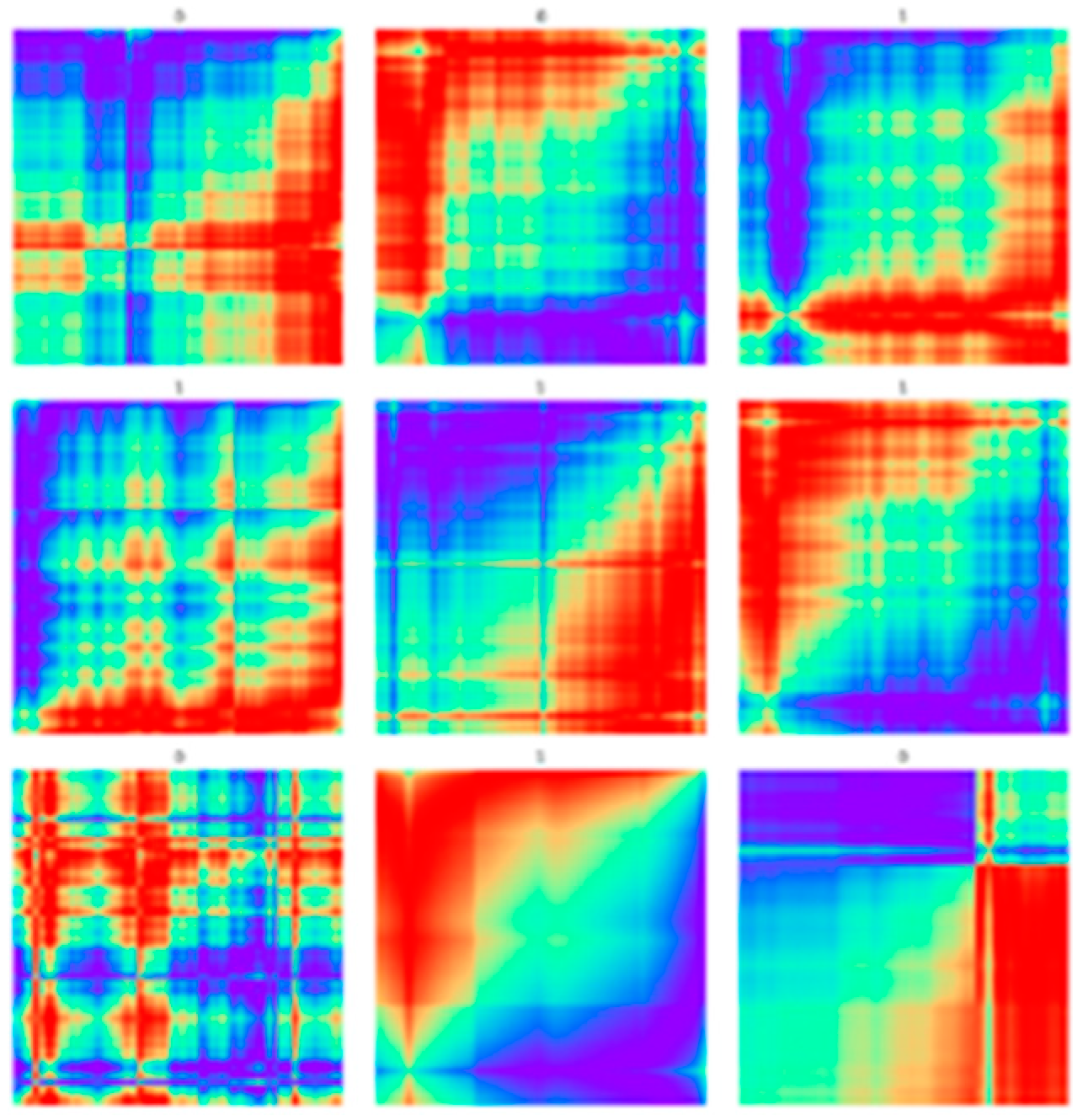
2.7. Image of Time Series by GADF

In preparing time series data, such as stock prices and trading volumes, for CycleGAN processing, a key step involves converting the data into 3D tensors [7,31]. This transformation utilizes the concept of the Gramian matrix from linear algebra, defined as the Hermitian matrix of inner products for a set of vectors in an inner product space [42].

The process begins by rescaling the time series data, denoted as X Subsequently, a coordinate transformation is applied, converting the data from Cartesian coordinates (represented as time stamp and data value pairs, (ti, xi)) to polar coordinates (represented by radius and angle, (ri, ϕi)) [42]. This transformation imparts two critical properties to the resulting map. Firstly, it is bijective, meaning each time series uniquely corresponds to one transformation result, attributable to the monotonicity of cos ϕ within the range [0, p] [42]. Secondly, it retains the absolute temporal relations of the original series. The outcome of this coordinate transformation on the rescaled time series data yields the Gramian angular difference field (GADF), as in Equation (1) [42]:

$$GADF=\left[sin\right(\varphi i-\varphi j\left)\right]=[sin\varphi icos\varphi j-cos\varphi isin\varphi j]=\sqrt{1-{X\prime }^2}X-X\prime \sqrt{1-X^2}$$

(1)

The Gramian angular difference field (GADF) is conceptualized as a Gramian matrix, with each element representing an inner product in the Gramian angular fields. However, it diverges from the traditional Gramian matrix in linear algebra due to a distinct definition of the inner product. By assigning varying colors to different values in the Gramian angular fields, time-series images are generated [42].

GADF is meant to transform the time series data, such as stock price and trading volume, into a three-dimensional image as shown in Figure 5. This study is the first one that uses GADF to transform the time series data of stock price and trading volume into 3D images, where the dimension N can be set to 64, determining the height and width (64 × 64) of the GADF time-series images, each with a depth of three channels for the colors as the third dimension of the transformed tensor. These images, derived from the SSE Composite Index’s daily closing data over the past 64 days, are used to predict future trends. An image is labeled ‘1’ if there is an average upward trend in the daily closing over the next five days compared to the past five days and ‘0’ otherwise. The dataset comprises 3314 images labeled ‘0’ and 3718 labeled ‘1’ for training and validation, along with 44 images labeled ‘0’ and 51 labeled ‘1’ in the test set. Figure 5 in this study displays examples of these GADF images. The correctness of GADF used for the transformation of a series of stock prices and trading volumes into 3D tensors is implied in the evaluation of the loss function of CycleGAN; that means that the loss function of CycleGAN will not converge when the transformation by GADF is not correct.

2.8. System Engineering (SE) and Dynamic Behavior

In his seminal work from 1972, Seely categorizes modules within system engineering and science into three fundamental classifications: physical, analytical, and descriptive [15]. Specifically, the analytical model employs mathematical principles to delineate the unique characteristics of a system. Typically, this model is articulated using simultaneous equations [15]. The current study incorporates various elements of this analytical module as Figure 6 to further its research objectives [15,16]. After the principle of system engineering, we can model the stock market as a simple harmonic motion system as illustrated by Figure 6.

• Mass: When considering Newton’s second law, the mass M relates to the formula:

f = M dv/dt = Ma, where M indicates mass, which is a relevant factor for the given problem; v denotes velocity; d presents the differential; t signifies the time; a represents the acceleration. It is imperative to establish associations among thrust (F), speed (v), and time (t);

2.

Damper (friction force): f = Dv; D is the friction constant, and v is the speed.

The force in question originates from deformation induced by force F, culminating in energy accumulation within the object. This phenomenon is instrumental in assessing whether resistance or deceleration factors are operative within the given environmental context. Pertinently, friction manifests through three principal mechanisms: static; Coulomb; and viscous friction. The present study focuses on static friction. Static friction is intrinsically linked to the commencement of motion and emerges at the juncture of contact between two surfaces;

3.

Spring (spring force): Accounting for spring pushback force (R). A spring is an element that stores mechanical potential energy through elastic deformation.

Formula: f = K∫vdt; K is the spring constant; v is the speed; d is the differential, and t is the time. ∫vdt represents displacement.

In the realm of stock prediction research, the incorporation of SE concepts has been undertaken through a multitude of approaches and perspectives. This research posits that the implementation of system dynamics within stock prediction merits additional investigation and empirical testing [16]. Employing experimental design, as clarified in the next section, this study aims to identify critical parameters of the problem and compute the ensuing forward distance, which will be elucidated in the subsequent section.

2.9. Active Learning and Design of Experiment (DoE)

2.9.1. Surrogate Function and Active Learning

In scientific and engineering domains, model design hinges on comprehensive performance analysis under varied design parameters, typically conducted through extensive, high-fidelity computer simulations, essential for pre-building insights into model performance, which are costly due to their number. Surrogate modeling, a data-driven strategy, is emerging as a solution to expedite these analyses [43]. It involves creating a surrogate model, also called metamodeling, a statistical representation that approximates the output of original simulations [44]. This model is then utilized for optimization, sensitivity, and risk analysis tasks, replacing the original simulation [41,45].

The surrogate model operates similarly to supervised ML, taking inputs and estimating outputs akin to simulation results [7,43]. This concept aligns with the training iterations in DL models. Surrogate modeling, a subset of supervised ML, particularly DL, focuses on training and validation to address issues like overfitting and underfitting [43].

Training a surrogate model involves careful selection of design parameter samples, encompassing two phases: generating observed points using DoE techniques akin to parameter selection and fitting the model to the data [43,44]. The distribution of these samples critically influences the model’s predictions. Hence, identifying informative points for model accuracy with minimal samples is a key challenge, such that the information ratio becomes out of the question.

Active learning enhances the training process by directing the next sample to where the surrogate model’s prediction error is the greatest [43]. The expected prediction error in ML is composed of bias and variance, often assessed through MSE [7,8]. With limited simulation runs, cross-validation is used to estimate the bias term [7,43], and additional methodologies, such as DoE, are employed to optimize sample selection for active learning [43,44].

2.9.2. DoE and Taguchi Method

Dr. Genichi Taguchi’s experimental design method, introduced in the 1950s, revolutionized the experimental approach with its use of orthogonal arrays [46]. This method, popularized globally by the 1980s and commonly known as the Taguchi method, efficiently determines the impact of various parameters on outcomes through Signal-to-Noise (S/N) ratio and variance analyses [47]. The S/N ratio particularly aids in reducing the effects of noise on parameter selection, expediting the identification of optimal settings, and enhancing product quality [46].

The Taguchi method necessitates the distinction between control factors, i.e., variables under experimental control, and noise factors, i.e., uncontrollable elements. For instance, in ceramics, control factors include ingredient ratios and firing methods, whereas environmental conditions act as noise factors [48]. Selecting an orthogonal array is pivotal based on the control factor count. This array selection, illustrated through the Latin square method, defines the structure of experiment groups [47]. The L8(2⁷) array, for example, means eight groups, two levels for each control factor, and seven control factors in total.

The final stage involves using the S/N ratio to identify the most effective control factor levels. This ratio calculation seeks to minimize noise impact while emphasizing controllable factors’ influence. The selection of a specific S/N ratio method is contingent upon the unique demands of each experiment [46,47].

$$\mathrm{Larger}\text{-}\mathrm{the}\text{-}\mathrm{Better}\mathsf{\eta }=-10\ast \mathrm{l}\mathrm{o}\mathrm{g}({\displaystyle \frac{1}{n}}\ast {\sum }_{i=1}^n{\displaystyle \frac{1}{y_i^2}})$$

$$\mathrm{Smaller}\text{-}\mathrm{the}\text{-}\mathrm{Better}\mathsf{\eta }=-10\ast \mathrm{l}\mathrm{o}\mathrm{g}({\displaystyle \frac{1}{n}}\ast {\sum }_{i=1}^n{y}_i^2)$$

$$\mathrm{Nominal}\text{-}\mathrm{the}\text{-}\mathrm{Better}\mathsf{\eta }=10\ast \mathrm{l}\mathrm{o}\mathrm{g}\left({\displaystyle \frac{{ysumofaverage}^2}{S^2}}\right)$$

In the realm of experimental design, the SN ratio is a pivotal metric, where ‘n’ corresponds to the number of experimental results; ‘y’ encapsulates the derived values, and ‘S’ represents their standard deviation. The magnitude of the SN ratio is inversely proportional to result variability. After calculation, SN ratios for each parameter level within an orthogonal array are aggregated and averaged. The parameter level with the maximal SN ratio is then identified as the most advantageous for the given experiment [49].

Notably, the utilization of the Taguchi Method in parameter optimization for DNNs has been substantiated by various studies [48]. This methodology enhances efficiency in parameter selection while reducing the experimental trials needed. Furthermore, it guarantees a certain standard of quality, significantly benefiting both the training process and the prediction accuracy of the DNNs [48].

2.10. Bollinger Bands

Developed by American financial analyst John Bollinger in 1980, Bollinger Bands is a technical analysis tool that employs moving averages and statistical standard deviations [1,2,50]. This methodology generates three key lines: upper; middle; and lower bands, as shown in Figure 7 [50,51]. The middle band is calculated as the moving average of the stock price over a predetermined time period as the blue curve in the upper part of Figure 7, commonly set at 20 days [51]. The upper band is formulated by adding twice the standard deviation of the stock price to the middle band as the red curve of the upper part of Figure 7, while the lower band is derived by subtracting twice the standard deviation from the middle band as the green curve in the upper part of Figure 7 [50].

These bands serve as indicators of market volatility and price trends. When the stock price nears the upper band, it often suggests a potential price decline, signifying overbought conditions. Conversely, approaching the lower band indicates oversold conditions, hinting at a possible price increase. The bands, therefore, act as dynamic levels of support and resistance, providing insights into the stock’s trading range and potential price-turning points [50,51].

(1)

Middle band

The formula of the simple moving average for N time period is

$$SMA={\displaystyle \frac{{(P}_1+P_2+P_3+\dots +P_n)}{n}}$$

where P is the stock price;

(2)

Upper band: Standard deviation of the middle band + K × N time period;

(3)

Lower band: Middle track-standard deviation of K × N time period;

(4)

Extended index—%b index: The position of the closing price in the Bollinger Bands is presented in digital form as a key indicator for trading decisions. The formula is

$$\mathrm{\%}\mathrm{b}={\displaystyle \frac{\mathrm{c}\mathrm{l}\mathrm{o}\mathrm{s}\mathrm{e}-\mathrm{l}\mathrm{o}\mathrm{w}\mathrm{e}\mathrm{r}\mathrm{b}\mathrm{a}\mathrm{n}\mathrm{d}}{\mathrm{u}\mathrm{p}\mathrm{p}\mathrm{e}\mathrm{r}\mathrm{b}\mathrm{a}\mathrm{n}\mathrm{d}-\mathrm{l}\mathrm{o}\mathrm{w}\mathrm{e}\mathrm{r}\mathrm{b}\mathrm{a}\mathrm{n}\mathrm{d}}}$$

$$\mathrm{B}\mathrm{a}\mathrm{n}\mathrm{d}\mathrm{w}\mathrm{i}\mathrm{d}\mathrm{t}\mathrm{h}={\displaystyle \frac{\mathrm{u}\mathrm{p}\mathrm{p}\mathrm{e}\mathrm{r}\mathrm{b}\mathrm{a}\mathrm{n}\mathrm{d}-\mathrm{l}\mathrm{o}\mathrm{w}\mathrm{e}\mathrm{r}\mathrm{b}\mathrm{a}\mathrm{n}\mathrm{d}}{\mathrm{m}\mathrm{i}\mathrm{d}\mathrm{d}\mathrm{l}\mathrm{e}\mathrm{b}\mathrm{a}\mathrm{n}\mathrm{d}}}$$

The %b value, integral to Bollinger Bands analysis, quantifies the stock’s closing price position relative to the bands, often extending beyond the nominal range of 0 to 1 [50]. A %b value greater than 1 signifies that the closing price exceeds the upper band, indicative of an upward trend shift. In contrast, a %b value of less than 0 implies that the closing price is below the lower band, signaling a downward trend shift. Analyzing the %b indicator is crucial for investment decisions as it offers insights into market trends and the relative strength or weakness of the stock, guiding traders in making informed decisions [51]. It employs predictive analytics, projecting stock prices onto the Bollinger Bands’ three levels for the next day. When the prediction suggests a higher future stock price, it may indicate that the current price is relatively low, implying a potential delay in selling, as indicated by the Sharp Ratio, which is often used in combination with the Markowitz Model for investment with bargaining analysis.

2.11. Evaluation and Experimental Results

This study employs four distinct models to predict and assess future stock prices [3,7,26]:

• MSE (Mean Squared Error): This model computes the mean of the squares of the differences between actual and predicted values. MSE serves dual purposes; it evaluates the model’s accuracy and optimizes the gradient for neural network convergence. Under a consistent learning rate, a lower MSE correlates with a smaller gradient, indicating improved model performance [3,7];
• MAE (Mean Absolute Error): MAE calculates the mean of the absolute differences between actual and output values. This metric provides a more direct representation of the discrepancy between predicted and real values, thereby effectively gauging the precision of the predictive model [3,7];
• Accuracy and Precision [26,39].

The Confusion Matrix, shown in

Table 1. Confusion Matrix.

	Predicted Stock Price Is Rising	Predicted Stock Price Is Falling
Actual Stock Price is rising	True Positive (TP)	False Negative (FN)
Actual Stock Price is falling	False Positive (FP)	True Negative (TN)

, a crucial tool in ML classification, comprises rows and columns that align predicted outcomes with actual results, enabling an assessment of model performance [26,39]. Integral to this evaluation is the F1 Score, which harmonizes precision and recall into a singular metric for accuracy assessment. Key components of this analysis include the following [26]:

(1)

Accuracy: Defined as the proportion of true results; i.e., both true positives and true negatives) among the total number of cases examined. It is calculated as (TP + TN)/(TP + FP + FN + TN). However, accuracy may be misleading, especially in cases of class imbalance;

(2)

Precision: This measures the ratio of true positives to the total prediction positives, calculated as TP/(TP + FP). Precision, sometimes conflated with accuracy, specifically refers to the consistency of repeated measurements under unchanged conditions;

(3)

Recall (sensitivity): Also known as the true positive rate, recall evaluates the model’s ability to correctly identify positive instances. The F1 Score, derived as 2TP/(2TP + FP + FN), is the harmonic mean of precision and recall, ranging from 0.0 (worst) to 1.0 (best). It is especially useful in scenarios where both recall and precision are crucial;

(4)

Return on Investment (ROI): ROI quantifies the efficiency of an investment, calculating the proportionate return relative to the investment cost [25]. In predictive modeling, ROI helps assess the financial benefit yielded by models like Bollinger Bands.

ROI = ((Investment Gain)/(Investment Base))

3. Research Method

3.1. Development Framework

The overall development program is illustrated in Figure 8 This study’s methodology is executed using Python and PyTorch, with the ReLU as the activation function, Adam as the optimizer, and Cross-Entropy for loss calculation in our proposed model. Initially, a web crawler collected stock data from January 2012 to December 2022, focusing on the semiconductor industry from the Taiwan Securities Exchange (TWSE), which is the authority body for security exchange in Taiwan. This dataset is then processed through a CycleGAN to analyze the joint effect of stock price and trading volume. The objective is to discern any significant patterns or differences between these two variables. Insights derived from this analysis are subsequently utilized in another predictive model, which aims to predict future stock prices and assess the accuracy of these predictions through error analysis.

3.2. Data Set

• Data Source: TWSE;
• Stock data: TSMC (2330.TW);
• Historical data: closing price and trading volume on each trading day;
• Data interval: January 2012 to December 2022, a total of ten years of trading day data;
• Training data: the first 90% of the total data is used as the training set, and 10% of the total data is used as the validation set;
• Test data: the last 10% of the total data.

3.3. Active Learning and DoE

In this experiment, we further define the following hyperparameters:

• Learning rate (CycleGAN GAN, ${\mathrm{l}\mathrm{r}}_{\mathrm{c}\mathrm{y}\mathrm{c}\mathrm{l}\mathrm{e}}$): CycleGAN Model Learning Rate;
• Learning rate (Prediction, ${lr}_p$): Learning Rate of the Prediction Model;
• λ_cls: Tuning the hyperparameters of L_cls in CycleGAN;
• λ_res: Tuning the hyperparameters of L_res in CycleGan;
• T: Represents the variation in data from the past T days utilized for predictions by model P;
• D: Indicates the data prediction D days into the future.

In the subsequent phase, the format of the data grouping is delineated in

Table 2. Schematic diagram of data format.

Daily change in trading volume on T days. Daily change in closing price on T days

Transaction Volume Label Closing price Label Political Factors Label Economic Factors Label

. Herein, ‘T’ signifies the number of days encompassed in the time series data. Additionally, each T-day data segment is assigned to a specific label group, as defined in the table. The data format, following this categorization, is structured in a manner detailed below:

To integrate the joint effect of trading volume and price exchange into the model, this study employs CycleGAN to discern the stock price and volume joint effect. In detail, the model is structured so that when the trading volume label is assigned a value of 0, the corresponding stock price label is set to 1, and the temporal data for the closing price are marked as 0, as delineated in

Table 3. Schematic diagram of transaction volume data format.

Daily change in trading volume on T days. Daily change in closing price on T days

Trading volume Label [0] Political factors Label Economic factors Label

. Inversely, when the transaction price label is ascribed a value of 1, the trading volume label is concurrently set to 0, with the associated time series data for the trading volume being zeroed, as illustrated in

Table 4. Schematic diagram of single stock price data format.

Daily change in trading volume on T days. Daily change in closing price on T days

[0] Transaction price Label Political factors Label Economic factors Label

.

Owing to the complexities in evaluating and procuring data that include political and economic elements as described in Section 2.2, this investigation centers singularly on the joint impact of stock price and volume, serving as labels for the dual components of the CycleGAN. The dataset, in its entirety, is methodologically structured into a group, which is then sequentially fed into the neural network at regular intervals spanning T days. This dataset is subsequently divided, allocating 80% for training purposes and 20% for testing. Furthermore, the experiment incorporates the setting of two distinct levels for each of the six hyperparameters, as elaborately detailed in

Table 5. Taguchi method L8(2⁶) parameter level.

Level	T	D	${\mathit{\lambda }}_{\mathit{c}\mathit{l}\mathit{s}}$	${\mathit{\lambda }}_{\mathit{r}\mathit{e}\mathit{s}}$	${\mathit{l}\mathit{r}}_{\mathit{C}\mathit{y}\mathit{c}\mathit{l}\mathit{e}}$	${\mathit{l}\mathit{r}}_{\mathit{p}}$
1	25 day	1 day	0.8	250	0.001	0.001
2	30 day	5 day	1	200	0.0005	0.0005

.

Next, various experimental groups are combined through the Taguchi method orthogonal table as in

Table 6. Taguchi method L8(2⁶) experimental combination.

No. of Experiments	T	D	${\mathit{\lambda }}_{\mathit{c}\mathit{l}\mathit{s}}$	${\mathit{\lambda }}_{\mathit{r}\mathit{e}\mathit{s}}$	${\mathit{l}\mathit{r}}_{\mathit{c}\mathit{y}\mathit{c}\mathit{l}\mathit{e}}$	${\mathit{l}\mathit{r}}_{\mathit{p}}$
1	1	1	1	1	1	1
2	1	1	1	2	2	2
3	1	2	2	1	1	2
4	1	2	2	2	2	1
5	2	1	2	1	2	1
6	2	1	2	2	1	2
7	2	2	1	1	2	2
8	2	2	1	2	1	1

:

Following the initial phase, this study identifies the optimal six sets of hyperparameters. This selection is followed by a subsequent experimental phase, wherein these chosen hyperparameters are applied. The efficacy of this model under these refined conditions is then meticulously evaluated using a pre-defined validation process.

3.4. Data Pre-Processing

To handle the missing data for holidays, we set the absent data unchanged from the day before.

3.4.1. Normalization of Stock Prices and Trading Volumes

This research addresses the disparate value ranges between stock price and trading volume by employing a two-step normalization process. The difference between the two values will be too large, which will affect the operation of the CycleGAN. Initially, the data undergo transformation into change rates, followed by a logarithmic adjustment to bridge the value gap. Subsequently, the min–max normalization technique is applied, ensuring all data values fall within the 0 to 1 range.

In this methodology, X represents the original dataset, encompassing variables like closing price and trading volume. The transformed data are denoted as Z, with max–max(X) and min–min(X) indicating the highest and lowest values in the dataset over a decade. The min–max normalization, applied to both trading volume and stock price, scales all stock values from various companies within the same industry to a unified range of 0 to 1. This standardization facilitates the model’s analysis of industry-wide trends and characteristics.

The min–max formula utilized is as follows:

$$zi={\displaystyle \frac{xi-min\left(x\right)}{max\left(x\right)-min\left(x\right)}}$$

where zi is the normalized value. xi is the value to be normalized. min(x) is the minimum value in the data. max(x) is the maximum value in the data.

Following this, the daily variation in the data is computed using a simple subtraction method:

∆Zi = Zi − Z_i−1

3.4.2. Direct Normalization

This study applies the min–max normalization technique to all dataset variables except for market capitalization. To accommodate the unique role of market capitalization as a divisor in subsequent system dynamics simulations, a tailored normalization approach is employed. This involves a specific transformation formula that adjusts the normalized values of market capitalization to range between 0.5 and 1. This strategic adjustment preserves the integrity of the simulation process and precludes computational anomalies that may arise from a divisor value of zero.

$$zi={\displaystyle \frac{xi+1}{2}}$$

3.5. Training/Validation/Test Data

To mitigate the risk of overfitting in the model, the dataset is strategically partitioned into three distinct segments. The time series data are allocated as follows: 90% for the training set; 10% for the validation set; and the last 10% of the training set is designated as the test data since the time series data are sequential in order of time. This division ensures a comprehensive evaluation of the model’s performance across different data subsets, enhancing its generalizability and robustness.

3.6. Deep Learning Architecture

3.6.1. Design of CycleGAN

In order to learn the joint effect of stock price and trading volume, this study uses CycleGAN, as shown in Figure 9; the core mechanism is the Cycle loss, and its loss function is calculated as follows:

$$L_{cyc}(G,F)=E_{x\sim pdata\left(x\right)}\left[\right|\left|F\right(G\left(x\right))-x|{|}_1]+E_{y\sim pdata\left(y\right)}[\left|\right|G\left(F\right(y\left)\right)-y\left|{|}_1\right].$$

For each image from the domain, the method to transform the joint effect of the domain learning trading volume and stock price, that is, return to the original image through the loop mechanism, is as follows:

x→G(x)→F(G(x)) ≈ x

Another core mechanism of the CyclicGAN is to combat loss, and its loss function is as follows:

$$L_{GAN}(G,D_Y,X,Y)=E_{y\sim pdata\left(y\right)}\left[log{D}_Y\right(y\left)\right]+E_{x\sim pdata\left(x\right)}\left[log\right(1-D_Y\left(G\right(x\left)\right)]$$

Among them, G tries to make the generated image G(x) look like a picture from the Y field and tries to distinguish Dy between the converted sample G(x) and the sample of the real Y field. The goals of this network are

$$L(G,F,D_X,D_Y)=L_{GAN}(G,D_Y,X,Y)+L_{GAN}(F,D_X,Y,X)+\lambda L_{cyc}(G,F)$$

Finally, to solve: $G^{\mathrm{*}},F^{\mathrm{*}}=arg\begin{array}{c}min\\ G,F\end{array}\begin{array}{c}max\\ D_x,D_Y\end{array}L(G,F,D_x,D_Y)$.

In this research, stock price and trading volume are utilized as inputs for the CycleGAN. The data are initially transformed into three-dimensional, image-like structures using the GADF method. The network architecture integrates CNN with a 48-block ResNet, which is a pre-trained model of ResNet, functioning as the generator. This generator creates outputs sophisticated enough to challenge the discriminator, which also employs a CNN framework to distinguish between authentic training data and synthetic outputs produced by the generator. The CycleGAN’s effectiveness hinges on the ResNet’s ability to intricately extract features and it is designed to be 48 layers, with a focus on a five-day period determined through DoE for reconstructing stock prices and trading volumes. This study emphasizes the adaptation of CycleGAN from its original image-focused application to the analysis of financial data. The stock price and trading volume are transformed into three-dimensional matrices feeding to FC layers, serving as inputs for both the generative and discriminative models in the CycleGAN framework, as illustrated in Figure 9.

3.6.2. Stock Price Prediction Models

This study employs the SE approach, as illustrated in Figure 10, to model stock market volatility, specifically examining the joint effect of stock price and trading volume. It posits that the CycleGAN’s synthetic outputs, denoted as G(x) and F(y) as shown in Figure 11, mirror potential future trends in these two variables. The model conceptualizes the joint effect of stock price and trading volume as a dynamic process akin to the transformation of potential energy into kinetic energy. This conceptual framework is intended to capture the driving forces behind stock price movements, thereby offering insights into market dynamics.

(1)

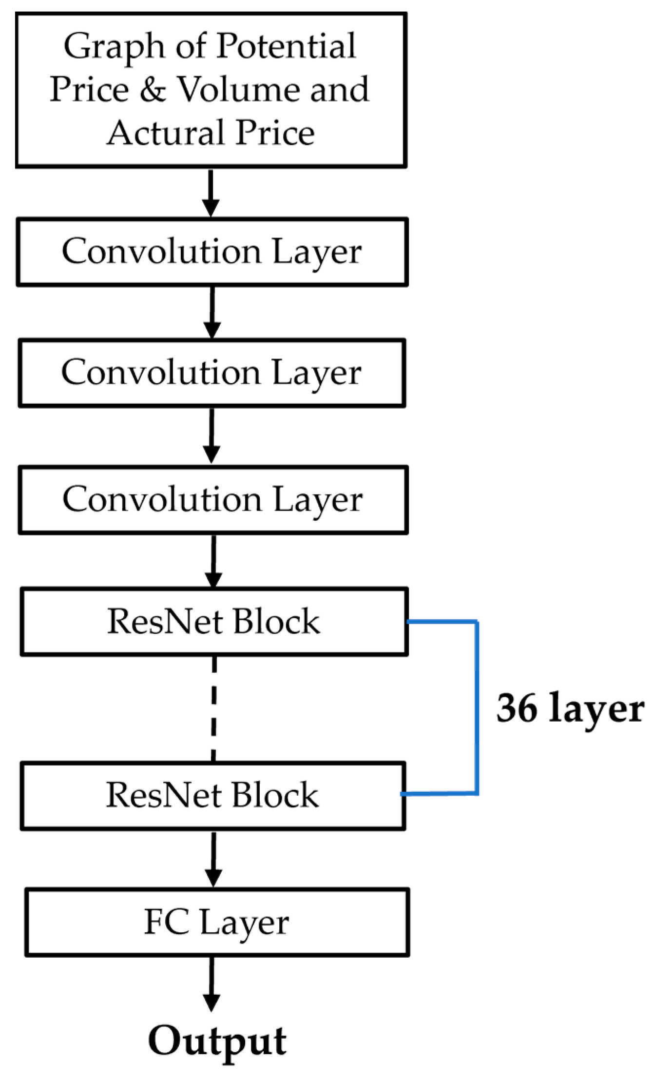
CNN + ResNet Architecture: This approach integrates CNN for eigenvalue extraction with a ResNet framework. Specifically, the model utilizes a 36-day stock price reduction period, determined by the DoE, to inform the architecture of the ResNet. Consequently, the ResNet is structured with 36 layers, a design choice illustrated in Figure 12;

(2)

LSTM Model: The LSTM model is employed to reconstruct time series data related to stock prices. In this configuration, a five-day period (also determined by the DoE) encompassing stock price and trading volume data is utilized. The LSTM model is accordingly designed with four layers, as depicted in Figure 13.

3.7. System Engineering and Dynamics

To simulate stock market dynamics, this study defines key elements as follows:

(1)

Force (F): Computed as the product of market value (M) and the displacement value predicted by the model. F represents the external capital’s influence on market value. The input variables, Xt and Yt, are derived from the potential and current stock prices and trading volumes, respectively. These variables simulate the energy thrust of the market;

(2)

Market Value (M): Calculated as the product of closing stock price and the number of issued stocks. A change in market value reflects how capital inflows affect stock price growth rates across different market capitalizations;

(3)

Friction (f): Represented as a function of transaction tax (set at 3% in Taiwan), calculated from the product of trading volume, stock price, and the tax rate. It represents the resistance encountered during stock transactions.

(4)

Resilience (R): Based on the stock’s previous day’s performance, resilience correlates with the potential energy stored in the stock price movement. It is modeled to reflect the principle of the Bollinger Bands, with the rebound force increasing as the stock price deviates from its average;

(5)

Acceleration (a): Derived using a distance formula, assuming an initial velocity of zero. It is calculated based on the stock price at a specified future time point.

The theoretical force (F) is adjusted for friction (f) and resilience (R) to calculate the actual force influencing the market. The displacement value output by the model is adjusted for gravity (g) and the transaction tax rate to yield the actual displacement value, representing the market movement.

According to the above assumptions, the output of the prediction model is displacement, so the Theoretical F can be calculated as follows:

F = M × (Displacement value output by the model)/d²t

Friction exerts a force in the opposite direction, so when F is positive, f is negative. And because the normal force needs to be calculated to calculate the kinetic friction force, the acceleration due to gravity is set to g, and the friction coefficient is 0.003 (transaction tax).

f = |M × g| × 0.003

The spring pushback force increases in proportion to the deviation from the mean, utilizing the closing price as the computational standard. The magnitude of the spring pushback force is determined with reference to two standard deviations. Additionally, the parameter denoted as λ_R is introduced as an adjustment factor for the spring pushback force. Consequently, the formulated expression for the spring pushback force in this study is given by

R = λ_R × M × (Displacement value output by the model)/d² × |(Bollinger Bands Average-Stock closing price for the day)/(Bollinger Bands Standard Deviation × 2)|

The simulation system dynamics formula used in this study is combined as follows:

Theoretical F-f-R = actual F

The simplified formula is

Displacement value output by the model: (g × 0.003) − (λ_R × Displacement value output by the model × |(Bollinger Bands Average-Stock closing price for the day)/(Bollinger Bands Standard Deviation × 2)|) = Actual displacement value, displacement value output by the model ≥ 0.

3.8. Design of Bollinger Band

The extended indicator, %b, derived from Bollinger Bands, serves as a pivotal trading signal, facilitating the assessment of near-future stock price strength. This indicator enables traders to discern whether the current stock price is at a relatively high or low point in recent times, thus informing trading decisions. The %b indicator is calculated in relation to the Bollinger Bands, providing a quantifiable measure of a stock’s price relative to its upper and lower bounds as follows:

(1)

Upper band: middle band + standard deviation of K × N time period;

(2)

Lower band: Middle band-standard deviation of K × N time period.

The Bollinger Bands typically set K at 2 and N at 20. This configuration is derived from the rule of normal distribution, where approximately 95% of the values are contained within a range of two positive and negative standard deviations from the mean;

(3)

Extended Indicator—%b Indicator: The %b value, a numerical metric, quantifies the closing price’s relative position within the Bollinger Bands, thereby serving as a critical index for informed trading decisions. Specifically, a %b value of 0.5, or 50% in percentage terms, indicates that the closing price is precisely at the midpoint of the Bollinger Bands. The value of %b is calculated as

((Upper Bollinger Band − Lower Bollinger Band)/(Closing Price − Lower Bollinger Band))

The %b indicator, an essential tool in Bollinger Band analysis, lacks pre-defined upper and lower limits due to the closing price’s potential to oscillate beyond the band range of 0 to 1. A %b value exceeding 1 indicates an upward trend breach, with the closing price above the upper band. Conversely, a %b value below 0 signifies a downward trend breach, where the closing price falls beneath the lower band. Analyzing the %b indicator is instrumental for investment decision-making, providing critical insights into market conditions and guiding strategic actions such as buying or selling based on the indicator’s demonstrated strengths or weaknesses.

Trading decisions using Bollinger Band can be described as follows:

(1)

Select the closing price of the day;

(2)

The three-band setting parameter K is obtained by experimenting with Bollinger Bands. Two experiments are used to obtain the K that can make it have the best average reporting rate;

(3)

The closing price fluctuates between the upper and lower bands, with its magnitude occasionally surpassing the band range (0 to 1). Consequently, the %b value does not possess a definite boundary. When there is an upward trend break, and the closing price situates above the upper band, the %b value exceeds 1; inversely, during a downward trend break with the closing price below the lower band, the %b value is less than 0. By scrutinizing and analyzing the ‘%b Indicator’, investors can gain insights to inform their trading decisions based on the indicator’s prevailing momentum. The three-band setting parameter N is also obtained through experimental Bollinger bands, experiments 5~35, interval 5, and the parameter N that can make it have the best average reporting rate is obtained;

(4)

When setting the %b indicator ≥ 1, the stock should be sold (if it has not been bought before, it will not be sold). The stock should be bought when the %b index ≤ 0. The research methodology was implemented using PyTorch.

4. Results of the Experiments and Evaluation

4.1. Parameter Selection

Utilizing the Taguchi method’s orthogonal table, eight distinct experimental combinations were developed. These were implemented using TSMC’s stock data spanning from January 2012 to December 2022. Each of the eight experiments offered insights into the learning trajectory of the generator, discriminator, and predictive models, including analyses via Bollinger Band and comparisons of actual versus predicted trends. The training phases demonstrated a consistent decrease in loss, culminating in a stable convergence, thereby signifying the models’ effective learning. Additionally,

Table 7. Experimental results of Taguchi method experimental combination (MAE).

	Trading Volume	Closing Price
1	0.0840	0.0084
2	0.0838	0.0080
3	0.0964	0.0171
4	0.0937	0.0167
5	0.0884	0.0085
6	0.0865	0.0081
7	0.0976	0.0161
8	0.0936	0.0175

delineates the MAE corresponding to each experimental setup. To ensure uniformity, all numerical data were subject to min–max normalization.

In this study, the stock’s closing price is the primary metric, with an emphasis on achieving lower values, thereby establishing a minimization goal. The noise factor in the experiment is represented by a single computer, assigned the variable n = 1. As a result, the SN ratio is calculated with the objective of minimizing the closing price, as detailed in

Table 8. SN ratio for minimizing the closing price.

Test Group	1	2	3	4	5	6	7	8
SN Ratio	41.51	41.94	35.34	35.55	41.41	41.83	35.86	35.14

.

Utilizing the Taguchi method’s framework, the SN ratio averages were calculated for each designated level, as detailed in

Table 9. Taguchi method parameter average SN ratio at each level.

	T	D	${\mathit{\lambda }}_{\mathit{c}\mathit{l}\mathit{s}}$	${\mathit{\lambda }}_{\mathit{r}\mathit{e}\mathit{s}}$	${\mathit{l}\mathit{r}}_{\mathit{c}\mathit{y}\mathit{c}\mathit{l}\mathit{e}}$	${\mathit{l}\mathit{r}}_{\mathit{p}}$
Level 1	38.59	41.67	38.61	38.53	38.46	38.40
Level 2	38.56	35.47	38.53	38.62	38.69	38.74
Contribution (max–min)	0.03	6.2	0.08	0.09	0.23	0.34
Factor importance ranking	6	1	5	4	3	2
Decision Level	1	1	1	2	2	2

. The experimental level exhibiting the highest average SN ratio was then identified and selected as the optimal parameter for the ensuing experimental procedures.

The finally decided parameters are shown in the

Table 10. Optimal parameters.

T	D	${\mathit{\lambda }}_{\mathit{c}\mathit{l}\mathit{s}}$	${\mathit{\lambda }}_{\mathit{r}\mathit{e}\mathit{s}}$	${\mathit{l}\mathit{r}}_{\mathit{s}\mathit{t}\mathit{a}\mathit{r}}$	${\mathit{l}\mathit{r}}_{\mathit{p}}$
25	1	0.8	200	0.0005	0.0005

:

Employing the Taguchi method for parameter optimization, this study’s model demonstrates proficiency in predicting stock market data a day in advance, effectively utilizing a dataset encompassing a 25-day period.

4.2. Single Stock Prediction of Semiconductor Industry

In the preliminary phase, this study employed data from TSMC spanning January 2012 to October 2022 for training and testing purposes. This dataset was processed utilizing parameters refined via the Taguchi method. The outcomes of these tests, as delineated in

Table 11. TSMC stock test results drawing of data of 2010-01~2022-10 (MAE).

Trading Volume	Closing Price
0.0805	0.0077

, reveal a noteworthy finding: the model’s error rate in predicting closing prices stands at approximately 0.77.

In the subsequent phase of this research, data spanning from June 2012 to May 2022 were harnessed as the training and testing dataset. This dataset was processed using parameters refined via the Taguchi method. The outcomes of the testing phase are systematically presented in

Table 12. TSMC stock test results drawing of data of 2012-06~2022-05 (MAE).

Trading Volume	Closing Price
0.0816	0.0056

, showcasing the performance and efficacy of the selected parameters.

In this study’s second phase, semiconductor stock data from the post-2019 pandemic period were analyzed, yielding a notably low prediction error of approximately 0.56% for closing prices. This study’s system dynamics formula necessitates the parameters g and λ_R. Unlike the conventional gravitational constant g (9.8), in the stock market context, g was set to 1 for this experiment. The parameter λ_R was meticulously adjusted to evaluate its impact. The findings, detailed in

Table 13. Testing Results of Five Semiconductor Companies. Stocks (2012-01 to 2022-10, MAE)

Transaction Volume	Opening Price	Highest Price	Lowest Price	Closing Price
0.0426	0.0042	0.0045	0.0037	0.0047

, amalgamate data from key semiconductor stocks, notably TSMC, spanning January 2012 to October 2021 and apply system dynamics principles.

The experimental findings, as detailed in

Table 14. TSMC single-strand system dynamics experiment combination (2010-01~2020-10).

Test Group	g	${\mathit{\lambda }}_{\mathit{R}}$	Trading Volume	Closing Price
1	-	-	0.0805	0.0077
2	1	0.01	0.0773	0.0073
3	1	0.04	0.0732	0.0068
4	1	0.05	0.0735	0.0067
5	1	0.06	0.0747	0.0067
6	1	0.07	0.0768	0.0066
7	1	0.08	0.0792	0.0067
8	1	0.09	0.0822	0.0067
9	1	0.1	0.0860	0.0068

, reveal that setting the parameters g = 1 and λ_R = 0.07 resulted in a reduction in the prediction error by approximately 0.11%. This outcome implies the effectiveness of the predictive model developed in this study, which integrates SE. The experiment combined data from key players in the semiconductor industry, particularly TSMC, covering the period from June 2012 to May 2021, and applied the principles of system dynamics to achieve these results.

The experimental outcomes, as delineated in

Table 15. TSMC single-strand system dynamics experiment combination (2011-06~2021-05).

Test Group	g	${\mathit{\lambda }}_{\mathit{R}}$	Trading Volume	Closing Price
1	-	-	0.0816	0.0056
2	1	0.01	0.0786	0.0053
3	1	0.04	0.0748	0.0048
4	1	0.05	0.0748	0.0047
5	1	0.06	0.0756	0.0047
6	1	0.07	0.0775	0.0047
7	1	0.08	0.0800	0.0047
8	1	0.09	0.0830	0.0048
9	1	0.1	0.0864	0.0049

, demonstrate that implementing parameters g = 1 and λ_R = 0.07 results in a marginal decrease in prediction error, approximately 0.09%. These findings suggest that the predictive model employed in this research, which integrates system dynamics, achieves a noteworthy degree of accuracy and effectiveness.

4.3. Multi-Stock Forecasting in the Semiconductor Industry

As described in Section 2.2, we have extended our methodology for the prediction of multiple stocks simultaneously and utilized stock data from Taiwan’s semiconductor industry, spanning from January 2012 to October 2022, including TSMC and four other randomly selected semiconductor companies, for a total of five companies. The test results are shown in the figure below.

The experimental results show that this model achieves an error margin of approximately 0.47% in predicting closing prices. Compared to single-stock forecasts, this model is better suited for predicting multiple stocks, making it advantageous for portfolio management of investment using the Sharpe Ratio.

4.4. Results of Experiment of Learning Joint Effect of Stock Price and Trading Volume with CycleGAN

From Figure 14, it can be observed that the loss of Generator G, Generator F, and the Cycle loss decreases significantly as the number of epochs increases. It is assumed that Cycle loss functions as a hyperparameter, and after training it to a certain level, further raining is halted.

Based on

Table 16. CycleGAN loss (MSE).

Days	Training Cycle Loss	Valid Cycle Loss	Testing Cycle Loss
20	0.031995635	0.038789876	0.036866438
25	0.016229397	0.016477194	0.015846474
30	0.0015571207	0.031062838	0.030280465

, it can be observed that the CycleGAN architecture effectively captures the relationship between volume and price. The testing results show a significant reduction in Cycle loss, indicating that the model successfully learns the volume-price relationship through the CycleGAN. Using 25-day volume and price data as input yields the lowest loss values as shown in Table 16. The training, validation, and testing Cycle loss values are all minimized, with minimal variation between them. Therefore, the neural network parameter n is set to 25, as previously mentioned, to optimize the model’s performance.

4.5. Performance of the Prediction of the Stock Price

Validation of Predictive Model

The predictive model’s accuracy is quantified using the MSE, where a lower MSE value, approaching zero, signifies greater precision. In this study, a network architecture combining CNN and ResNet was implemented. The model’s efficacy was thoroughly assessed through key performance metrics, notably the F1 Score and Accuracy, as detailed in Figure 15. These metrics provide a comprehensive understanding of the model’s predictive capabilities.

The analysis with a 25-day time frame, as shown in Figure 15, reveals that the model’s optimum performance is achieved with a five-day prediction horizon, confirming the result of DoE, evidenced by a 59% average accuracy in predicting stock price direction and a high F1 score. This result underscores the model’s proficiency in discerning patterns pertinent to five-day predictions determined by DoE. In contrast, one-day predictions exhibit reduced performance, reflecting the model’s limited ability to adapt to very short-term fluctuations. Additionally, ten-day predictions yield lower accuracy, possibly due to a misalignment with the data timeframe and lesser correlation. Comparatively, the CNN and ResNet integration surpasses the LSTM model in both accuracy and F1 Score for five-day predictions, indicating a stronger capability in detecting weekly market trends. It is notable, however, that LSTM shows its best performance in terms of F1 score for ten-day predictions, illustrating its effectiveness in integrating longer-term data.

4.6. Performance of Stock Price Prediction by Using Normalization

Stock price prediction performance is significantly influenced by factors such as data normalization and the incorporation or exclusion simulation of SE, each contributing distinct benefits. In the context of DNN applied to linear regression, normalization of target data is a common practice. This strategy aims to mitigate the occurrence of excessively large loss values, which could elongate convergence times or, in some instances, inhibit convergence entirely. However, this study encountered various challenges after the application of normalization to the target data.

Within the realm of linear regression DNNs, normalizing target data is a standard practice aimed at curbing excessive loss values. This approach is employed to avert prolonged periods of convergence or to forestall scenarios of non-convergence. Nevertheless, this study encountered multiple challenges after the normalization of target data.

Normalization Restoration Discrepancies: The target data, originating from daily stock price variations and further modified in the simulated SE framework by division by the square of the number of days, result in exceedingly small values. This leads to potential discrepancies in the data post-normalization restoration, diverging from the initial dataset.

Pre- and Post-Normalization Data Discrepancy in linear regression: The original data range, extending from −1.8 to 2.3, suggests that significant discrepancies between pre- and post-normalization data are improbable. Hence, the chances of extended convergence periods or non-convergence in the linear regression model are minimal.

4.7. Performance of Stock Price Prediction Integrating of Dynamic SE Simulation

The effectiveness of stock price prediction relies on the application of normalization and the integration of dynamic SE simulation, as shown in

Table 17. MAE by the prediction of stock price with ResNet.

	Training	Validation	Testing	Average
ResNet, no SE and Normalization	1.951394	3.345	5.097	3.464465
ResNet, with SE, no Normalization	3.211395	4.104	5.3906	4.235332
ResNet, no SE, with and Normalization	1.9069737	3.9998	5.3466	3.37511246
ResNet, with SE and Normalization	15.592605	9.153	12.2104	12.318668

and

Table 18. MAE by the prediction of stock price with LSTM.

	Training	Validation	Testing	Average
LSTM no SE and Normalization	1.995237	3.38	5.0802	3.485146
LSTM, with SE, no Normalization	3.5186053	3.7602	5.3088	4.1958684
LSTM no SE, and Normalization	2.002026	3.356	5.073	3.477009
LSTM, with SE and Normalization	11.24382	13.5698	18.6598	14.49114

.

(1)

Within the dynamic SE simulation, ResNet demonstrates enhanced learning for normalized target data, outperforming LSTM. Conversely, in scenarios lacking normalization, LSTM exhibits better performance;

(2)

Excluding the dynamic SE simulation, normalized target data lead to lower training losses but increased validation and test losses, adversely affecting ResNet’s outcomes more than LSTM;

(3)

Overall, when combined with dynamic SE simulation, LSTM outshines ResNet, displaying more consistent losses across training, validation, and test stages, with an average loss of 4.1958684 compared to ResNet’s 4.235332. Without simulation integration, ResNet matches LSTM’s performance, showing little variation in loss metrics;

(4)

Ultimately, ResNet, when used without simulation of system engineering and non-normalized target data, achieves the most accurate stock price prediction with the least deviation, marking a superior result of 3.464465.

4.8. Trading Signals and the ROI Prediction by Bollinger Band

With N set to 35 and K designated as 2, the optimal reporting rate is obtained as follows.

4.8.1. Trading Signal of Bollinger Band

This study presents a novel integration of stock price prediction with Bollinger Bands to evaluate a stock’s current price strength. A predicted lower future price suggests that the current price is high, prompting immediate selling actions. A significant observation, detailed in Figure 16, Figure 17, Figure 18, Figure 19 and Figure 20, is the diminished trading frequency with this method compared to traditional Bollinger Band strategies. This lower frequency of trades reflects a more cautious investment approach, supported by improved accuracy in price prediction.

4.8.2. ROI

The ultimate goal of this approach is to enhance ROI by fine-tuning trading strategies based on forward-looking insights. The Bollinger Bands method, particularly its %b index extension, has proven effective in guiding stock market investment strategies. However, these developments show that integrating this method into stock price prediction models significantly enhances ROI as demonstrate d in

Table 19. Table of Return on Investment by Various Methods.

Method.	Training	Validation	Testing	Total Average
Bolinger Band	0.140962	0.20709	0.121204	0.155066
Prediction by LSTM combined with SE and Bolling Band	0.191472	0.227625	0.123423	0.19198
Prediction by ResNet combined with SE and Bolling Band	0.209931	0.228786	0.123423	0.203827
Prediction by LSTM combined with Bolling Band, no SE	0.156184	0.229696	0.124331	0.1698
Prediction by ResNet combined with Bolling Band, no SE	0.17589	0.262105	0.124331	0.189294

. Empirical findings reveal that combining Bollinger Bands with the LSTM model under simulation of system engineering increases average ROI to 19.1%, while integration with the ResNet model yields 20.3%. In the absence of simulation of system engineering, the ROI with LSTM is 16.9%, and with ResNet, it is 18.9%. These figures notably exceed the original Bollinger Bands’ average ROI of 15.5%, which is the effect of coupling system engineering with Bollinger Band to capture the price movement in the short term. Such integration leverages prediction insights, allowing investors to make more informed decisions by identifying whether the current stock price is relatively high or low, both presently and in the foreseeable future.

5. Conclusions

This research proposes a CycleGAN, incorporating ResNet as the generator and CNN as the discriminator, designed to analyze and predict stock prices by learning the joint effect of stock price and volume. Utilizing TSMC’s stock data, the CycleGAN output, seen as a disturbance to stock prices, is fed into deep learning models, specifically ResNet and LSTM, for prediction. Recognizing the stock market as a nonlinear dynamic system, the research couples these DL models with the Simple Harmonic Motion model, adhering to Newton’s second law, to predict short-term stock prices. Additionally, the predicted stock prices from various models are analyzed using Bollinger Bands to determine the trading frequency and expected ROI, aiding investment decisions. These DL models serve as surrogate functions for statistical tools and sensitivity and risk analyses, to optimize model training and prevent overfitting or underfitting, active learning via the Taguchi method is employed. Overall, this research is the first of its kind. Key findings and contributions include the following:

• This pioneering research uses CycleGAN with ResNet and CNN to analyze the stock price–volume joint effect, demonstrating its effectiveness in estimating potential prices and volumes. A notable reduction in cycle loss was achieved, with the lowest loss recorded for the 25-day stock price and trading volume determined by DoE;
• The optimal configuration, comprising a 25-day data interval for CycleGAN and a five-day prediction period, determined by DoE, led to superior outcomes, evidenced by elevated accuracy and F1 scores. In stock price prediction, ResNet surpassed LSTM in terms of accuracy and precision;
• This study investigates the incorporation of the outcomes from CycleGAN learning and predictive DL models into system engineering based on the assumption that future trading volume and price differing from current values will impact subsequent stock prices. This concept was tested within a system engineering framework. The analysis suggests that using the predictive model for future price and volume trends and integrating these into the system engineering framework enhances the accuracy of stock price predictions, as indicated by a lower error rate in the latter method compared to the former;
• Further research evaluated the effectiveness of combining stock price prediction with Bollinger Bands over a five-day span. The findings show that Bollinger Bands, enriched with predictive model data, outperform those based solely on historical information. This approach led to a reduced frequency of trading signals and a 30% increase in average ROI, highlighting the potential of system engineering in resolving challenges in the stock market domain and contributing to the field.

Reflecting on the limitations of this research, we outline prospective enhancements and future research directions:

• In terms of DL, this study utilized ResNet within CycleGAN for stock price prediction. Future research should expand this approach by incorporating Inception as well as DenseNet, even potentially an ensemble of the above three DL tools, i.e., ResNet, Inception, and DenseNet, into CycleGAN and stock price predictions. Additional parameters may also be integrated to improve this model’s performance;
• Surprisingly, ResNet’s stock price prediction performance surpasses that of LSTM, which is traditionally used for time series analysis, such as stock price prediction. Consequently, future investigations could explore the use of Gated Recurrent Units (GRU) as an alternative to LSTM for enhanced stock price prediction;
• Regarding trading strategies, the current reliance on Bollinger Bands and the %b index as trading signals should evolve. Future strategies will incorporate diverse trading signals, including frequency analysis through Wavelet, to synergize with stock price predictions;
• Although coupling DL with system engineering improves stock price prediction with higher accuracy and expected ROI, the impact of system engineering regarding precision is not consistently significant. This may be due to CycleGAN’s learning the joint effects of stock price and volume, reflecting stock market dynamics. Stock trading is often viewed through the lens of cash flow dynamics. Therefore, future models may benefit from adopting a fluid mechanics perspective rather than the current solid body approach to better simulate the flow of financial assets;
• Starting from collecting foreign stock data to compare whether the Taiwanese domestic and foreign markets have the same effect or the domestic stocks with lower trading volume to further verify the versatility of this method.

References

- DeMark, T.R. The New Science of Technical Analysis; John Wiley and Sons, Inc.: Hoboken, NJ, USA, 1984. [Google Scholar]
- ADAM HAYES. Technical Analysis Definition. Available online: https://www.investopedia.com/terms/t/technicalanalysis.asp (accessed on 1 January 2022).
- Chiang, J.K.; Gu, H.Z.; Hwang, K.R. Stock Price Prediction based on Financial Statement and Industry Status using Multi-task Transfer Learning. In Proceedings of the International Conference on Information Management (ICIM), Taipei, Taiwan, 27–29 March 2020. [Google Scholar]
- Chen, S.W.; Wei, C.Z. The Nonlinear Causal Relationship between Price and Volume of Taiwanese Stock and Currency Market. J. Econ. Manag. 2006, 2, 21–51. [Google Scholar]
- Ying, C.C. Stock Market Prices and Volumes of Sales. Econometrica 1966, 34, 676–685. [Google Scholar] [CrossRef]
- Karpoff, J.M. The relation between price changes and trading volume: A survey. J. Financ. Quant. Anal. 1987, 22, 109–126. [Google Scholar] [CrossRef]
- Sri, L.M.; Yogesh, K.; Subramanian, V. Deep Learning with PyTorch 1.x, 2nd ed.; Packt Pub: Birmingham, UK, 2019. [Google Scholar]
- Gibson, A.; Patterson, J. Deep Learning, 1st ed.; O’Reilly Media, Inc.: Sebastopol, CA, USA, 2016. [Google Scholar]
- Goodfellow, I.J.; Pouget-Abadie, J.; Mirza, M.; Xu, B.; Warde-Farley, D.; Ozair, S.; Aaron, C.; Bengion, Y. Generative Adversarial Networks. arXiv 2014, arXiv:1406.2661. [Google Scholar]
- Wikipedia. Generative Adversarial Network. 2021. Available online: https://en.wikipedia.org/wiki/Generative_adversarial_network (accessed on 15 January 2022).
- Bruner, J. Generative Adversarial Networks for Beginners. 2023. Available online: https://github.com/jonbruner/generative-adversarial-networks/blob/master/gan-notebook.ipynb (accessed on 15 January 2022).
- Zhu, J.Y.; Park, T.; Isola, P.; Efros, A.A. Unpaired Image-to-Image Translation Using Cycle-Consistent Adversarial Networks. In Proceedings of the IEEE International Conference on Computer Vision, Venice, Italy, 22–29 October 2017; pp. 2223–2232. [Google Scholar]
- He, K.; Zhang, X.; Ren, S.; Sun, J. Deep Residual Learning for Image Recognition. In Proceedings of the IEEE Conference on Computer Vision and Pattern Recognition, Las Vegas, NV, USA, 27–30 June 2016; pp. 770–778. [Google Scholar]
- Hochreiter, S.; Schmidhuber, J. Long short-term memory. Neural Comput. 1997, 9, 1735–1780. [Google Scholar] [CrossRef] [PubMed]
- Hiemstra, C.; Jones, J.D. Testing for linear and nonlinear Granger causality in the stock price-volume relation. J. Financ. 1994, 49, 1639–1664. [Google Scholar]
- Seely, S. An Introduction to Engineering Systems; Pergamon Press Inc.: Tarrytown, NY, USA, 1972. [Google Scholar]
- MBA Knowledge Encyclopedia, System Dynamics. Available online: https://wiki.mbalib.com/zh-tw/%E7%B3%BB%E7%BB%9F%E5%8A%A8%E5%8A%9B%E5%AD%A6 (accessed on 1 October 2020).
- Taiwan’s TSMC controlled 60% of Foundry Market in Q1. Available online: https://www.taiwannews.com.tw/en/news/4917619 (accessed on 15 January 2022).
- Taiwan Economy Grows Fastest Since 2010 as TSMC Gives Boost. Available online: https://www.bloomberg.com/news/articles/2022-01-27/tsmc-s-40-billion-spree-may-tip-the-scales-on-taiwan-s-growth#xj4y7vzk (accessed on 1 January 2022).
- Yu, I.-Y. A Study on the Causal Relationship between Stock Prices and Trading Volume—Empirical Evidence from the Taiwan Stock Market. Master Thesis, Yoshimori University, Tokyo, Japan, 2021. [Google Scholar]
- Crouch, R.L. The volume of transactions and price changes on the New York Stock Exchange. Financ. Anal. J. 1970, 26, 104–109. [Google Scholar] [CrossRef]
- Stickel, S.E.; Verrecchia, R.E. Evidence that trading volume sustains stock price changes. Financ. Anal. J. 1994, 50, 57–67. [Google Scholar] [CrossRef]
- Sheu, H.J.; Wu, S.; Ku, K.P. Cross-sectional relationships between stock returns and market beta, trading volume, and sales-to-price in Taiwan. Int. Rev. Financ. Anal. 1998, 7, 1–18. [Google Scholar] [CrossRef]
- Tu, Y.P. The Relationship between Price and Volume under Taiwan’s Eight Major Stock indexes. Master Thesis, National Chengchi University, Taipei, Taiwan, 2016. [Google Scholar]
- Chiang, J.K.; Lin, C.L.; Chiang, Y.F.; Su, Y. Optimization of the spectrum splitting and auction for 5th generation mobile networks to enhance quality of services for IoT from the perspective of inclusive sharing economy. Electronics 2021, 11, 3. [Google Scholar] [CrossRef]
- Chiang, J.K.; Chen, C.C. Sentimental analysis on Big Data–on case of financial document text mining to predict sub-index trend. In Proceedings of the 2015 5th International Conference on Computer Sciences and Automation Engineering (ICCSAE 2015), Sanya, China, 14–15 November 2015; Atlantis Press: Paris, France, 2016; pp. 423–428. [Google Scholar]
- Sharpe, W.F. Capital Asset Prices: A Theory of Market Equilibrium under Conditions of Risk. J. Financ. 1964, 19, 425–442. [Google Scholar]
- Froot, K.A.; Perold, A.; Stein, J.C. Shareholder Trading Practices and Corporate Investment Horizons. Working Paper (No. 3638), National Bureau of Economic Research, February 1991. Available online: https://www.nber.org/papers/w3638 (accessed on 1 January 2022).
- Goodwin, T.H. The Information Ratio. Financ. Anal. J. 1998, 54, 34–43. [Google Scholar] [CrossRef]
- Chiang, J.K.; Lin, Y.S. Research into Optimization of Profit with Hedging for Stock Investment by Constructing Capital Asset Model with Simulated Annealing Method- with Example of 50 Stocks of 0050. In Proceedings of the International Conference of Information Management, Bandung, Indonesia, 13–14 August 2020. [Google Scholar]
- Zheng, Q.; Delingette, H.; Duchateau, N.; Ayache, N. 3D consistent biventricular myocardial segmentation using deep learning for mesh generation. arXiv 2018, arXiv:1803.11080. [Google Scholar]
- Wang, A. Backpropagation (BP). 2023. Available online: https://www.brilliantcode.net/1326/backpropagation-1-gradient-descent-chain-rule/ (accessed on 20 January 2022).
- LeCun, Y.; Boser, B.; Denker, J.S.; Henderson, D.; Howard, R.E.; Hubbard, W.; Jackel, L.D. Backpropagation applied to handwritten zip code recognition. Neural Comput. 1989, 1, 541–551. [Google Scholar] [CrossRef]
- Wikipedia. Convolutional Neural Network. 2022. Available online: https://en.wikipedia.org/wiki/Convolutional_neural_network (accessed on 15 January 2022).
- Zhang, L.; Aggarwal, C.; Qi, G.J. Stock price prediction via discovering multi-frequency trading patterns. In Proceedings of the 23rd ACM SIGKDD International Conference on Knowledge Discovery and Data Mining, Halifax, NS, Canada, 13–17 August 2017; pp. 2141–2149. [Google Scholar]
- Granger, C.W.; Morgenstern, O. Spectral analysis of New York stock market prices 1. Kyklos 1963, 16, 1–27. [Google Scholar] [CrossRef]
- Greff, K.; Srivastava, R.K.; Koutník, J.; Steunebrink, B.R.; Schmidhuber, J. LSTM: A search space odyssey. IEEE Trans. Neural Netw. Learn. Syst. 2016, 28, 2222–2232. [Google Scholar] [CrossRef] [PubMed]
- Hinton, G.E.; Salakhutdinov, R.R. Reducing the dimensionality of data with neural networks. Science 2006, 313, 504–507. [Google Scholar] [CrossRef] [PubMed]
- Townsend, J.T. Theoretical analysis of an alphabetic confusion matrix. Percept. Psychophys. 1971, 9, 40–50. [Google Scholar] [CrossRef]
- Sundermeyer, M.; Schlüter, R.; Ney, H. LSTM neural networks for language modeling. In Proceedings of the Thirteenth Annual Conference of the International Speech Communication Association, Portland, OR, USA, 9–13 September 2012. [Google Scholar]
- Gers, F.A.; Schmidhuber, J.; Cummins, F. Learning to forget: Continual prediction with LSTM. Neural Comput. 2000, 12, 2451–2471. [Google Scholar] [CrossRef] [PubMed]
- de Vitry, L. Encoding Time Series as Images-Gramian Angular Field Imaging. Analytics Vidhya, 15 October 2018. Available online: https://medium.com/analytics-vidhya/encoding-time-series-as-images-b043becbdbf3 (accessed on 1 January 2023).
- Guo, S. An Introduction to Surrogate Modeling, Part I: Fundamentals; Data Sci: Toronto, ON, Canada, 2020. [Google Scholar]
- Liu, H.; Cai, J.; Ong, Y.S. An adaptive sampling approach for Kriging metamodeling by maximizing expected prediction error. Comput. Chem. Eng. 2017, 106, 171–182. [Google Scholar] [CrossRef]
- Forrester, A.; Sobester, A.; Keane, A. Engineering Design via Surrogate Modelling: A Practical Guide; John Wiley & Sons: Berlin/Heidelberg, Germany, 2008. [Google Scholar]
- Plastics Industry Development Center of Taiwan, Quality Engineering. 2008. Available online: https://www.pidc.org.tw/safety.php?id=124 (accessed on 6 October 2022).
- Lee, H.H. Taguchi Methods: Principles and Practices of Quality Design, 4th ed.; Gao-Li Pub., 2022; Available online: https://www.studocu.com/tw/document/national-formosa-university/department-of-mechanical-and-computer-aided-engineering/taguchi-method-course/7369020 (accessed on 6 October 2022).
- Pan, Y.H. Application of the Taguchi Method in Neural Network Input Parameter Design—A Case Study on the Development of a Rapid Response System Model for Retailers. Master Thesis, Yoshimori University, Taiwan, 2003. [Google Scholar]
- Taguchi Quality Engineering, CH 9, Institute of Industry Engineering and Management. National Yunlin University of Science and Technology. Available online: https://www.iem.yuntech.edu.tw/lab/qre/public_html/Courses/1/AQM-1/files/CH9%20%E7%94%B0%E5%8F%A3%E6%96%B9%E6%B3%95.pdf (accessed on 6 October 2022).
- Bollinger, J. Using Bollinger Bands. Stock. Commod. 1992, 10, 47–51. [Google Scholar]
- CMoney. What is Bolinger Band. 2021. Available online: https://www.cmoney.tw/learn/course/technicals/topic/1216 (accessed on 6 October 2022).