Robo Advising and Investor Profiling

Abstract

The rise of digital technology and artificial intelligence has led to a significant change in the way financial services are delivered. One such development is the emergence of robo advising, which is an automated investment advisory service that utilizes algorithms to provide investment advice and portfolio management to investors. Robo advisors gather information about clients’ preferences, financial situations, and future goals through questionnaires. Subsequently, they recommend ETF-based portfolios tailored to match the investor’s risk profile. However, these questionnaires often appear vague, and robo advisors seldom disclose the methodologies employed for investor profiling or asset allocation. This study aims to contribute by introducing an investor profiling method relying solely on investors’ relative risk aversion (RRA), which, in addition, allows for the determination of optimal allocations. We also show that, for the period under analysis and using the same ETF universe, our RRA portfolios consistently outperform those recommended by the Riskalyze platform, which may suffer from ultraconservadorism in terms of the proposed volatility.

1. Introduction

In the current fast-paced technological landscape, companies are compelled to adapt swiftly and reinvent themselves. This rapid evolution extends to the asset-management service industry, where technological innovations, particularly in the form of robo advisors, have gained prominence.

Robo advising, also referred to as automated investment management or digital wealth management, has witnessed a significant surge in popularity within the investment sector. Its origins trace back to the early 2000s with the emergence of online investment platforms, but it entered a transformative phase in the mid-2010s. The first wave brought forth standalone digital investment platforms such as Betterment and Wealthfront, offering algorithm-driven portfolio management with low-cost ETFs and competitive fees. With the increasing popularity of robo advising, the second wave saw the entry of traditional financial institutions, including Vanguard, Charles Schwab, and Fidelity, providing their own digital investment services. In addition, some robo advisors adopted a hybrid model by partnering with financial advisors. This integration of digital and human advice allows investors to benefit from technology-driven portfolio management while retaining access to human guidance.

The evolution of robo advising has democratized access to investment management, rendering it more accessible and affordable for retail investors to build diversified portfolios [1]. For a thorough examination of the prepandemic evolution of robo advising and the associated regulatory landscape, ref. [2] provides a comprehensive overview. The COVID-19 pandemic has notably accelerated the adoption of algorithmic advice among bank clients, further propelling the digitization of the financial system [3]. Robo advising’s rising popularity is also attributed to convenience and user-friendly interfaces, particularly appealing to digital generations.

Despite its evolution and popularity, there has been a very limited number of studies comparing the performance of portfolios proposed by robos to traditional mutual funds. One exception is [4], but the main reason for the absence of studies is that robos do not disclose their portfolios, and in addition, they claim to tailor a portfolio for each investor, making it impossible to compare with traditional mutual funds. Another ambiguous aspect of robo advising lies in the evaluation of each investor’s risk profile. The assessment of risk preferences by robo advisors is undisclosed and often vague, exhibiting considerable differences across various platforms [5]. This is not surprising, as evaluating risk profiles is far from trivial, given that preferences for risk can vary significantly when measured by using different methods [6].

In this study, we look at actual robo portfolios proposed by Riskalyze—one of the most well-known US robo advisors—for three made-up profiles: conservative, moderate, and aggressive investors. The Riskalyze portfolios are the ones in [7]. Our main goals are (i) to assess the in-sample and out-of-sample performance of robo portfolios in comparison to mean-variance theory (MVT) optimal portfolios, and (ii) to advocate for the adoption of the relative risk aversion (RRA) measure for investor profiling. This objective measure of investor classification is exceptionally objective and enables the discrimination of investors beyond the traditional three broad classes.

The remainder of the paper is organized as follows. Section 2 presents an overview of the literature on robo advising. In Section 3, we detail the methodology and data used. Section 4 presents and discusses the results. Finally, Section 5 concludes the paper, highlighting the limitations of the analysis and suggesting avenues for further research.

2. Literature Review

This review delves into the emerging academic literature on robo advising, providing an overview of the existing research and the contextual landscape of robo analysis. Our paper contributes by attempting an empirical analysis and by presenting a tangible approach to investor profiling, adding a concrete dimension to the discussion.

Robo advising has experienced rapid expansion, driven by the integration of digital technology and a surge in passive investing. Reports indicate an annual growth rate of 24% since 2013, with projections suggesting the potential replacement of 47% of jobs in the next two decades [8]. As of 2020, robo advisors managed assets totaling USD 2.2 trillion, and this figure is anticipated to reach USD 16 trillion by 2025 [9]. The COVID-19 pandemic further accelerated the adoption of digital platforms [3,10]. Robo advisors offer advantages such as lower fees, diversified portfolios, and personalized advice. Lower fees can potentially lead to higher returns [4,11]. They excel in portfolio diversification, reducing investor risk [12]. Additionally, robo advisors provide personalized advice, mitigating behavioral biases [13,14].

Despite benefits, challenges include the absence of human interaction, impacting investor understanding and trust [15,16]. Algorithmic bias, particularly in recommending socially responsible investments, poses concerns [17]. Regulatory questions related to investor protection, compliance, and oversight also emerge [18]. The variability in risk profiling and portfolio allocation across robo advisors raises further questions [19]. The future of robo advising looks promising, with improving technology and increasing investor comfort. Integration with traditional advisory services is a potential growth area [20]. Artificial intelligence and machine learning may enhance personalization [21,22,23,24]. Expansion into financial planning, retirement planning, and banking services aims for a comprehensive financial suite. Advancements in data analytics, AI, and cybersecurity are crucial for enhanced efficiency and sophisticated advice [22].

In this study, we propose a method to classify investors based on the classical measure of relative risk aversion ($RRA$) from expected utility theory (EUT) [25]. We then evaluate the in-sample and out-of-sample performance of the robo portfolios proposed by Riskalyze, comparing them to our $RRA$ optimal portfolios and other classical MVT portfolios.

Although we consider directly various levels of $RRA$, there is some recent alternative literature on risk profiling that is worth mentioning. Ref. [26] proposes a method of measuring an investor’s risk appetite based on a ratio between risk-neutral and subjective probabilities. Ref. [27] presents an improved measurement of subjective risk tolerance and discusses its link to relative risk aversion. Ref. [28] suggests that robo advisors could use portfolio choices to learn investors’ risk preferences. Ref. [29] proposes a sophisticated model to evaluate the risk profile.

For further reading, we refer to the systematic literature review of [30] and to [31], which looks into the state-of-art in Fintech research and identifies gaps, challenges, and trends.

3. Methodology and Data

The objective of this study is to employ mean-variance theory (MVT) and expected-utility theory (EUT) to identify optimal portfolios for investors with varying levels of relative risk aversion ($RRA$). Subsequently, we compare the in-sample and out-of-sample performances of these $RRA$ optimal portfolios with those provided by Riskalyze for conservative, moderate, and aggressive investors.

3.1. Mean-Variance Portfolios

Given a set of risky assets, MVT allows one to find all efficient portfolios. That is, all portfolios with the biggest expected return for a given level of risk or with the least risk for a given level of expected return.

MVT is still the “standard” portfolio-building method, widely used not only by academics but also by practitioners [32]. Given a set of n risky assets with individual expected returns ${\overline{R}}_i$, for $i=1,\cdots ,n$, the expected return of any portfolio p is given by

$${\overline{R}}_p=\sum _{i=1}^n{x}_i{\overline{R}}_i$$

where $x_i$ shows the weight of each individual asset in a portfolio, and we have

$$\sum _{i=1}^n{x}_i=1.$$

The risk of a portfolio, as evaluated by the variance, is given by

$${\sigma }_p^2=var\left(R_p\right)=var\left(\sum _{i=1}^n{x}_i{R}_i\right)=\sum _{i=1}^n\sum _{j=1}^n{x}_i{x}_j{\sigma }_{ij}$$

where ${\sigma }_{ij}$ denotes the covariance between the returns of asset i and j.

In vector notation, we can use

$$\overline{R}=\left(\begin{array}{c}{\overline{R}}_1\\ {\overline{R}}_2\\ ⋮\\ {\overline{R}}_n\end{array}\right)\hspace{1em}X=\left(\begin{array}{c}{x}_1\\ x_2\\ ⋮\\ x_n\end{array}\right)\hspace{1em}V=\left(\begin{array}{cccc}{\sigma }_1^2& {\sigma }_{12}& \cdots & {\sigma }_{1n}\\ {\sigma }_{21}& {\sigma }_2^2& \cdots & {\sigma }_{2n}\\ ⋮& ⋮& \ddots & ⋮\\ {\sigma }_{n1}& {\sigma }_{n2}& \cdots & {\sigma }_n^2\end{array}\right)$$

(1)

and obtain

$$\begin{array}{c}\hfill {\overline{R}}_p=X^{\prime }\overline{R}{\sigma }_p^2=X^{\prime }VX\end{array}$$

(2)

In this study, we focus on MVT efficient portfolios: the tangent (T) portfolio, the minimum variance ($MV$) portfolio, as well as optimal portfolios for various levels of relative risk aversion ($RRA$).

Since we are considering that shortselling is not allowed (all robo portfolios seem to impose such a restriction), we must rely on numerical solutions to the following optimization problems.

3.1.1. Tangent Portfolio

The tangent (T) portfolio is, by definition, the one with the highest Sharpe ratio, so it solves

$$\begin{array}{cc}\hfill \underset{X}{max}& \frac{{\overline{R}}^{\prime }X-R_f}{\sqrt{X^{\prime }VX}},\hfill \\ \hfill \mathrm{s}.\mathrm{t}.& X^{\prime }\mathbf{1}=1\hfill \\ \hfill & x_i\ge 0\forall i\hfill \end{array}$$

where $\mathbf{1}$ denotes a vector of ones and the inequality restrictions impose no shortselling.

3.1.2. Minimum Variance Portfolio

The minimum variance (MV) portfolio solves

$$\begin{array}{cc}\hfill \underset{X}{min}& X^{\prime }VX,\hfill \\ \hfill \mathrm{s}.\mathrm{t}.& X^{\prime }\mathbf{1}=1\hfill \\ \hfill & x_i\ge 0\forall i.\hfill \end{array}$$

3.1.3. RRA Optimal Portfolios

We also consider optimal portfolios for investors with different levels of relative risk aversion ($RRA$). So, we take the investor’s perspective and analyze preferences. In modeling choice under uncertainty, we consider the EUT of Von Neumann and Morgenstern [25] to model economic agents’ decisions.

We start by recalling that for an investor with utility $U\left(W\right)$, twice differentiable, the relative risk aversion is defined by

$$\begin{array}{c}\hfill RRA\left(W\right)=-\frac{U^{″}\left(W\right)W}{U^{\prime }\left(W\right)}\end{array}$$

(3)

where W stands for the uncertain final wealth.

Also, given the uncertainty setup, the optimal portfolio for the investor is the one that maximizes expected utility at terminal wealth $\mathbb{E}\left[U\right(W\left)\right]$. Given the nonlinearity of most utilities, we consider a second-order Taylor approximation around initial wealth $W_0$:

$$\begin{array}{c}\hfill U\left(W\right)=U\left(W_0\right)+U^{\prime }\left(W_0\right)(W-W_0)+\frac{1}{2}{U}^{″}\left(W_0\right){(W-W_0)}^2.\end{array}$$

Making use of the notion of equivalent utility function, we can subtract $U\left(W_0\right)$ and divide by $U^{\prime }\left(W\right)>0$ and obtain the same preferences which we may choose to rewrite in terms of the return by using $W=(1+R)W_0$:

$$\begin{array}{c}\hfill U\left(R\right)=R{W}_0+\frac{1}{2}\frac{U^{″}\left(W_0\right)W_0}{U\left(W_0\right)}{\left(R\right)}^2{W}_0.\end{array}$$

Using once more the equivalence property (dividing by $W_0>0$) and the $RRA$ definition in Equation (3),

$$\begin{array}{c}\hfill U\left(R\right)=R-\frac{1}{2}RRA\left(W_0\right){\left(R\right)}^2,\end{array}$$

we obtain the utility to depend only on the uncertain return and the relative risk aversion evaluated at the initial wealth, which with a slight abuse of notation, we may write simply as $RRA$ (instead of $RRA\left(W_0\right)$).

The risk-tolerance function is nothing but $\mathbb{E}\left[U\right(W\left)\right]$, rewritten in terms of the mean-variance inputs:

$$\begin{array}{cc}\hfill f(\sigma ,\overline{R})& =\mathbb{E}\left[\tilde{U}\left(W\right)\right]\approx \overline{R}-\frac{1}{2}RRA\times \mathbb{E}\left[{\left(R\right)}^2\right]\approx \overline{R}-\frac{1}{2}RRA\left({\overline{R}}^2+{\sigma }^2\right)\hfill \end{array}$$

(4)

where $\overline{R}$ denotes the expected return and $\sigma$ the volatility.

One of the advantages of Equation (4) is that it only depends on the initial level of $RRA$ of investors. So, by varying $RRA$, we are able to capture very different profiles. For $RRA$ values between −1 and 6, we capture various investor profiles, from the risk lover ($RRA=-1$) to the risk-neutral ($RRA=0$) and all sorts of risk aversion with different degrees $RRA=1,2,3,4,5,6$. Empirical evidence seems to point to $0\le RRA\le 3$ as realistic levels of $RRA$ [33]. Here we go beyond those values of purpose to include all types of investors, from risk lovers to extreme risk aversion.

The optimal portfolio for a particular investor (with a particular level of $RRA$) solves the following problem:

$$\begin{array}{cc}\hfill \underset{X}{max}& {\overline{R}}_p-\frac{1}{2}RRA\left({\overline{R}}_p^2+{\sigma }_p^2\right),\hfill \\ \hfill \mathrm{s}.\mathrm{t}.& {\overline{R}}_p=X\prime \overline{R}\hfill \\ \hfill & {\sigma }_p=X^{\prime }VX\hfill \\ \hfill & X^{\prime }\mathbf{1}=1\hfill \\ \hfill & x_i\ge 0\forall i.\hfill \end{array}$$

3.2. Robo Portfolios

We have information only on three portfolios from Riskalyze, one for each broad classification of investors: conservative, moderate, and aggressive. The data for these portfolios come from [7], who on the 31 March 2017, by using real investments at the Riskalyze platform, obtained three portfolio compositions answering as conservative, moderate, and aggressive investors willing to invest for 5 years.

The aggressive investors are the ones that are enthusiastic about taking large amounts of risk and do not settle back when observing downward movements in their portfolios. They usually go for the risky asset classes, and when the market is performing well, they invest in the assets that present higher returns. Moderate investors are willing to take some risk, and they can handle it until observing a certain downward percentage in their portfolio, at which point they take their money. They usually invest part of their money in riskier assets and the other part in safer assets. Conservative investors are the ones that are hardly able to take any risk, so they always go for the safest assets, the ones that offer them capital protection, since they do not want to suffer losses. The risk tolerance of each investor is influenced by some determining factors, such as the financial situation, asset class preference, time horizon, and the purpose of the investment. Still, nowadays most robos rely on broad investor classifications such as the one they use.

3.3. Homogeneous Portfolio

In addition to the above-mentioned MVT and robo portfolios, we also consider the homogeneous H portfolio as a naïve benchmark.

3.4. Investment Strategy and Performance Evaluation

We conduct a comparative analysis of the performance of all the previously mentioned portfolios. The analysis begins with the estimation of the allocation to each asset. To do this, we invest USD 100 in each portfolio and observe how it evolves until maturity. We employ a monthly rebalancing strategy to realign the weightings of the portfolios. The choice of monthly rebalancing is based on findings from [34], which suggest that monthly rebalancing outperforms other strategies when unit transaction costs are below approximately 50 basis points and costs associated with ETFs are lower.

In addition to tracking the evolution, we compute the Sharpe ratio (SR) for each portfolio in both in-sample and out-of-sample periods as it is a commonly used performance metric. Apart from being a classical performance measure, ref. [35] highlights its connection to the “level of maximum expected utility provided by the asset”. This implies that when an asset exhibits a higher performance measure, it delivers a greater level of maximum expected utility.

The portfolio Sharpe ratio is defined as

$$\begin{array}{c}\hfill S{R}_p=\frac{{\overline{R}}_p-R_f}{{\sigma }_p}\end{array}$$

(5)

where ${\overline{R}}_p$ is the expected return of the portfolio, ${\sigma }_p$ is the volatility of the portfolio (as previously defined), and $R_f$ is the risk-free interest rate of the market.

3.5. Data

To carry out this study, we use data from

• The composition of three Riskalyze portfolios (conservative, moderate, and aggressive) on 31 March 2017, each designed for a 5-year investment horizon.
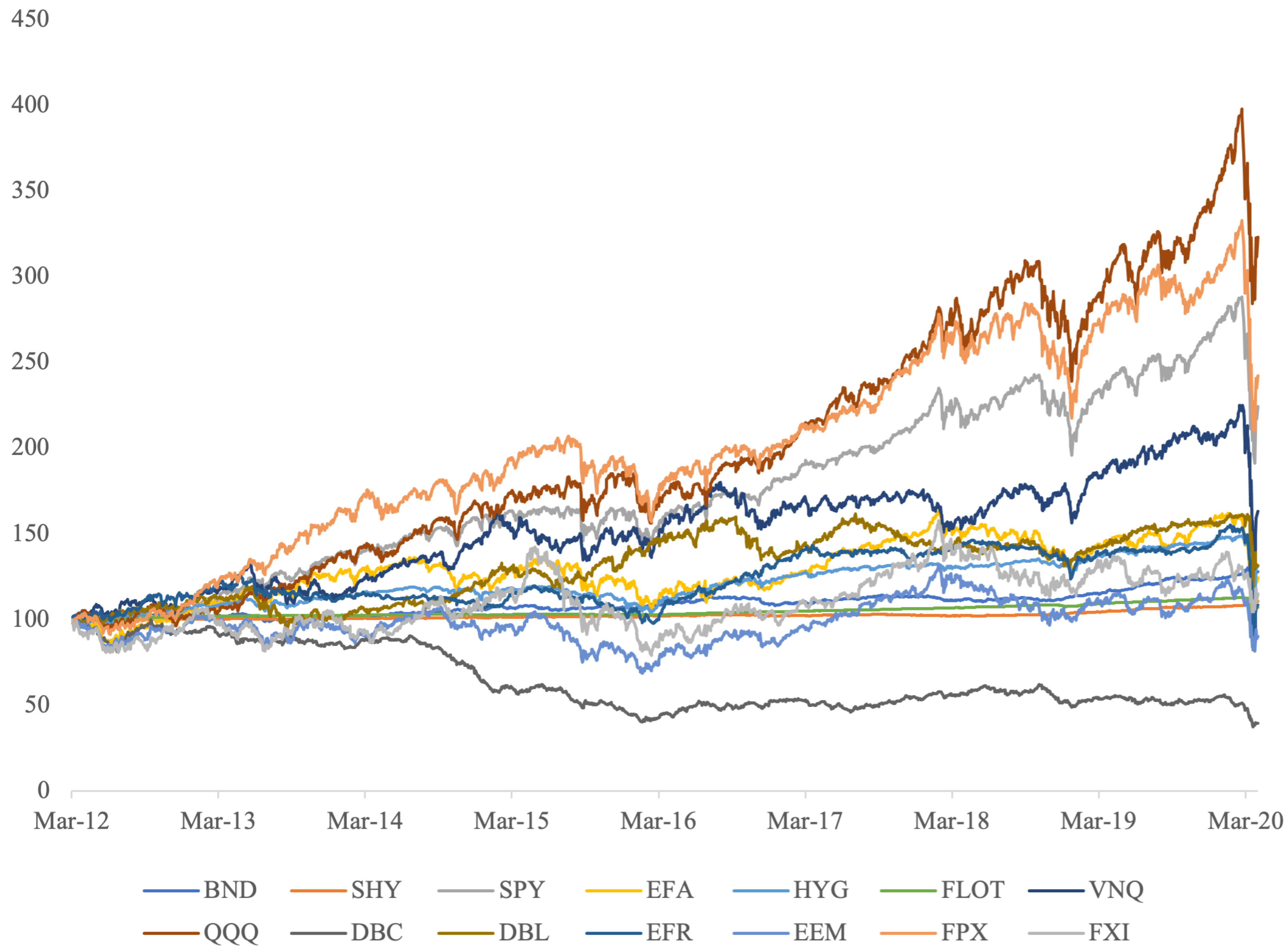
• Daily prices for all 15 ETFs included in the Riskalyze portfolio compositions, spanning from 1 April 2012 to 31 March 2020.

Table 1. Description, abbreviations, and categories of the 15 ETFs provided by the Riskalyze platform, which are used for the calculations in this study.

Index	Description	Category
BND	Vanguard Total Bond Market ETF	Intermediate-Term Bond
SHY	iShares 1-3 Year Treasury Bond	Short Government
SPY	SPDR S&P 500 ETF	Large Blend
EFA	iShares MSCI EAFE	Foreign Large Blend
HYG	iShares iBoxx USD High Yield Corporate Bd	High-Yield Bond
FLOT	iShares Floating Rate Bond	Ultrashort Bond
VNQ	Vanguard REIT ETF	Real Estate
QQQ	PowerShares QQQ ETF	Large Growth
DBC	PowerShares DB Commodity Tracking ETF	Commodities Broad Basket
DBL	Doubleline Opportunistic Credit Fund	Close-Ended Fixed-Income Mutual Fund
EFR	Eaton Vance Senior Floating-Rate Fund	Close-Ended Fixed-Income Mutual Fund
XLU	Utilities Select Sector SPDR ETF	Utilities
EEM	iShares MSCI Emerging Markets	Diversified Emerging Markets
FPX	First Trust US IPO ETF	Exchange-Traded Fund
FXI	iShares China Large-Cap	Exchange-Traded Fund

provides details on the ETFs, including descriptions, abbreviations, and categories. These are the ETFs proposed by Riskalyze in at least one of the portfolios under analysis. We consider “their” universe of assets and avoid entering a debate on why these assets were selected.

The in-sample calculations cover the initial 5-year period, from 1 April 2012 to 31 March 2017, while the out-of-sample performance evaluation spans from 1 April 2017 to 31 March 2020. The choice of concluding the out-of-sample period on 31 March 2020 aims to avoid potential bias from the impact of the COVID-19 pandemic crisis on our analysis. In addition to the 15 ETFs chosen by the platform, we also consider a risk-free asset, in this case the 5-year US Treasury Bond yields (0.16%).

Figure 1 presents the evolution of the prices of each ETF. At the very end of our sample (in March 2020), we still capture some of the COVID-19 impact.

We use the first 5 years of data to estimate the mean-variance inputs:

Table A1. In-sample expected returns and volatilities for all ETFs.

INDEX	$\overline{\mathit{R}}$	$\mathit{\sigma }$
BND	1.95%	3.22%
SHY	0.48%	0.78%
SPY	13.40%	12.63%
EFA	6.53%	15.55%
HYG	4.91%	6.62%
FLOT	0.98%	0.97%
VNQ	11.04%	14.77%
QQQ	16.27%	14.96%
DBC	−12.05%	14.70%
DBL	8.31%	13.81%
EFR	7.16%	10.38%
XLU	12.21%	13.88%
EEM	1.39%	19.20%
FPX	16.00%	15.51%
FXI	4.51%	23.22%

and

Table A2. In-sample variance–covariance matrix for all ETFs.

	BND	SHY	SPY	EFA	HYG	FLOT	VNQ	QQQ	DBC	DBL	EFR	XLU	EEM	FPX	FXI
BND	0.00104	0.00018	−0.0009	−0.00085	0.00006	−0.00001	0.00083	−0.00094	−0.00042	0.00094	−0.00007	0.00117	−0.00032	−0.001	−0.00097
SHY	0.00018	0.00006	−0.00023	−0.00018	−0.00003	0	0.00012	−0.00025	−0.00005	0.00011	−0.00006	0.00023	−0.00011	−0.00026	−0.00026
SPY	−0.0009	−0.00023	0.01595	0.01677	0.00577	0.00009	0.01189	0.01735	0.00726	0.00169	0.00352	0.00831	0.01874	0.01729	0.01897
EFA	−0.00085	−0.00018	0.01677	0.02419	0.00688	0.00013	0.01278	0.0178	0.0101	0.00203	0.00416	0.00869	0.0248	0.01814	0.0253
HYG	0.00006	−0.00003	0.00577	0.00688	0.00439	0.00003	0.00508	0.00605	0.00407	0.00156	0.00205	0.00331	0.00834	0.00644	0.00783
FLOT	−0.00001	0	0.00009	0.00013	0.00003	0.00009	0.00008	0.00007	0.0001	0.00002	0.00006	0.00005	0.00018	0.00008	0.0002
VNQ	0.00083	0.00012	0.01189	0.01278	0.00508	0.00008	0.02181	0.01195	0.00404	0.00442	0.00254	0.01284	0.01557	0.01258	0.01395
QQQ	−0.00094	−0.00025	0.01735	0.0178	0.00605	0.00007	0.01195	0.02238	0.00653	0.00208	0.00384	0.00742	0.02005	0.02013	0.02062
DBC	−0.00042	−0.00005	0.00726	0.0101	0.00407	0.0001	0.00404	0.00653	0.02159	0.00091	0.00234	0.00286	0.01352	0.00788	0.01202
DBL	0.00094	0.00011	0.00169	0.00203	0.00156	0.00002	0.00442	0.00208	0.00091	0.01908	0.00231	0.00333	0.00327	0.00197	0.00238
EFR	−0.00007	−0.00006	0.00352	0.00416	0.00205	0.00006	0.00254	0.00384	0.00234	0.00231	0.01077	0.00139	0.00453	0.00431	0.00462
XLU	0.00117	0.00023	0.00831	0.00869	0.00331	0.00005	0.01284	0.00742	0.00286	0.00333	0.00139	0.01927	0.01108	0.00727	0.00909
EEM	−0.00032	−0.00011	0.01874	0.0248	0.00834	0.00018	0.01557	0.02005	0.01352	0.00327	0.00453	0.01108	0.03685	0.0201	0.03779
FPX	−0.001	−0.00026	−0.00026	0.01814	0.00644	0.00008	0.01258	0.02013	0.00788	0.00197	0.00431	0.00727	0.0201	0.02406	0.02054
FXI	−0.00097	−0.00026	0.01897	0.0253	0.00783	0.0002	0.01395	0.02062	0.01202	0.00238	0.00462	0.00909	0.03779	0.02054	0.05392

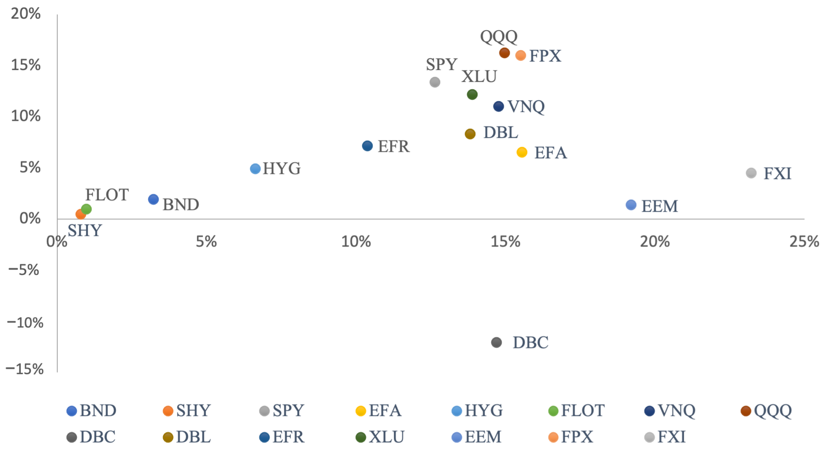
present the vector of expected returns and the variance–covariance matrix. Figure 2 shows the mean-variance representation of the ETFs. It considers only the in-sample data, so data before 31 March 2017, and we simply computed the historical averages and standard deviations of the returns by using a sample size equal to the investment horizon. This is information that Riskalyze had at the time they proposed their portfolios. Some of the recommended ETFs had performed particularly bad in the previous 5 years.

4. Results

4.1. In-Sample Results

Table 2. Compositions and basic statistics on the following portfolios: tangent (T); minimum variance (MV); homogeneous (H); and Riskalyze conservative (C), moderate (M), and aggressive (A).

	T	MV	H	C	M	A
BND	13.03%	0.00%	6.67%	35.00%	25.00%	0.00%
SHY	25.78%	61.81%	6.67%	30.00%	1.00%	0.00%
SPY	4.20%	0.64%	6.67%	13.00%	13.00%	26.00%
EFA	0.00%	0.00%	6.67%	5.00%	15.00%	20.00%
HYG	0.00%	0.00%	6.67%	5.00%	7.00%	0.00%
FLOT	51.37%	37.05%	6.67%	5.00%	0.00%	0.00%
VNQ	0.00%	0.00%	6.67%	2.00%	10.00%	12.00%
QQQ	0.00%	0.00%	6.67%	0.00%	5.00%	17.00%
DBC	0.00%	0.00%	6.67%	0.00%	5.00%	7.00%
DBL	1.13%	0.00%	6.67%	0.00%	7.00%	0.00%
EFR	1.32%	0.05%	6.67%	0.00%	7.00%	0.00%
XLU	0.00%	0.00%	6.67%	0.00%	5.00%	0.00%
EEM	0.00%	0.00%	6.67%	0.00%	0.00%	7.00%
FPX	3.17%	0.44%	6.67%	0.00%	0.00%	6.00%
FXI	0.00%	0.00%	6.67%	0.00%	0.00%	5.00%
${\overline{R}}_p$	2.14%	0.82%	6.21%	−0.02%	6.57%	9.32%
${\sigma }_p$	1.14%	0.59%	8.23%	2.88%	7.04%	12.80%
SR	1.732	1.126	0.735	−0.0609	0.9099	0.7158

and

Table 3. Compositions and basic statistics on optimal MVT portfolios for investors with $RRA=\left\{-1, 0, 0.5, 1, 1.25, 1.5, 2, 3, 4, 5, 6\right\}$.

RRA	−1.00	0.00	0.50	1.00	1.25	1.50	2.00	3.00	4.00	5.00	6.00
BND	0.00%	0.00%	0.00%	0.00%	0.00%	0.00%	0.00%	0.00%	0.00%	2.94%	20.36%
SPY	0.00%	0.00%	0.00%	0.00%	0.00%	0.00%	0.00%	37.98%	35.41%	29.39%	25.70%
QQQ	100%	100%	100%	100%	91.63%	85.76%	76.63%	0.00%	0.00%	0.00%	0.00%
DBL	0.00%	0.00%	0.00%	0.00%	0.00%	0.00%	0.00%	0.00%	13.38%	15.89%	12.47%
EFR	0.00%	0.00%	0.00%	0.00%	0.00%	0.00%	0.00%	0.00%	0.00%	10.35%	8.89%
XLU	0.00%	0.00%	0.00%	0.00%	0.00%	0.00%	2.79%	11.70%	14.33%	14.12%	9.65%
FPX	0.00%	0.00%	0.00%	0.00%	8.37%	14.24%	20.58%	50.32%	36.87%	27.31%	22.93%
${\overline{R}}_p$	16.27%	16.27%	16.27%	16.27%	16.25%	16.23%	16.10%	14.57%	13.51%	12.15%	10.36%
${\sigma }_p$	14.96%	14.96%	14.96%	14.96%	14.85%	14.79%	14.47%	11.62%	10.16%	8.84%	7.26%
SR	1.077	1.077	1.077	1.077	1.0836	1.0871	1.1022	1.2400	1.3136	1.3569	1.4045

present all the portfolio compositions and basic (in-sample) statistics.

Not surprisingly, from Table 2 and Table 3, we see that when we impose shortselling restrictions, the MVT portfolios end up investing in a limited number of ETFs. But so do the Riskalyze portfolios with the conservative investing in 7 ETFs, the moderate in 10 ETFs, and the aggressive in 8 ETFs.

Optimal portfolios according to $RRA$ vary from 100% invested in the highest-expected-return ETF (for the risk lovers, risk-neutral, and risk-averse up to $RRA=0.5$) to a maximum of six ETFs out of a set of just seven ETFs for all the other $RRA$ values. There are a few ETFs that are common across the two types of portfolios’ compositions. For instance, both the robo aggressive portfolio, A, and the $RRA$ portfolios with $RRA<2$ invest in QQQ and FPX, the difference being that while the robo portfolio invests in other ETFs, the $RRA$ portfolios are concentrated in those two ETFs. Moderate and conservative robo portfolios, M and C, share with RRA portfolios with $RRA=5 \mathrm{or} 6$ their investment in BND and SPY but then differ in how they invest in the other ETFs, with $RRA$ portfolios proposing a relatively high weight in FPX and DBL where robos invest marginally (and only in the moderate portfolio).

In terms of statistics, we see that the tangent portfolio T does maximize the Sharpe ratio but at the cost of low volatility and expected returns. The homogeneous portfolio has an expected return around 6% with a volatility around 8%, so a Sharpe ratio around 0.7. H does better on both dimensions than the Riskalyze conservative portfolio C, worse than the moderate portfolio M, and in line with the aggressive portfolio A. The Riskalyze Sharpe ratios are −0.0609, 0.9099, and 0.7158, for C, M, and A, respectively.

However, the portfolios that are optimal according to $RRA$ are the ones with relatively high Sharpe ratios for realistic levels of expected returns and volatility. All Sharpe ratios range from 1.0770 to 1.4045, increasing with the level of risk aversion. The expected returns and volatility decrease for increasing $RRA$s, but the expected returns decrease proportionally less than volatilities.

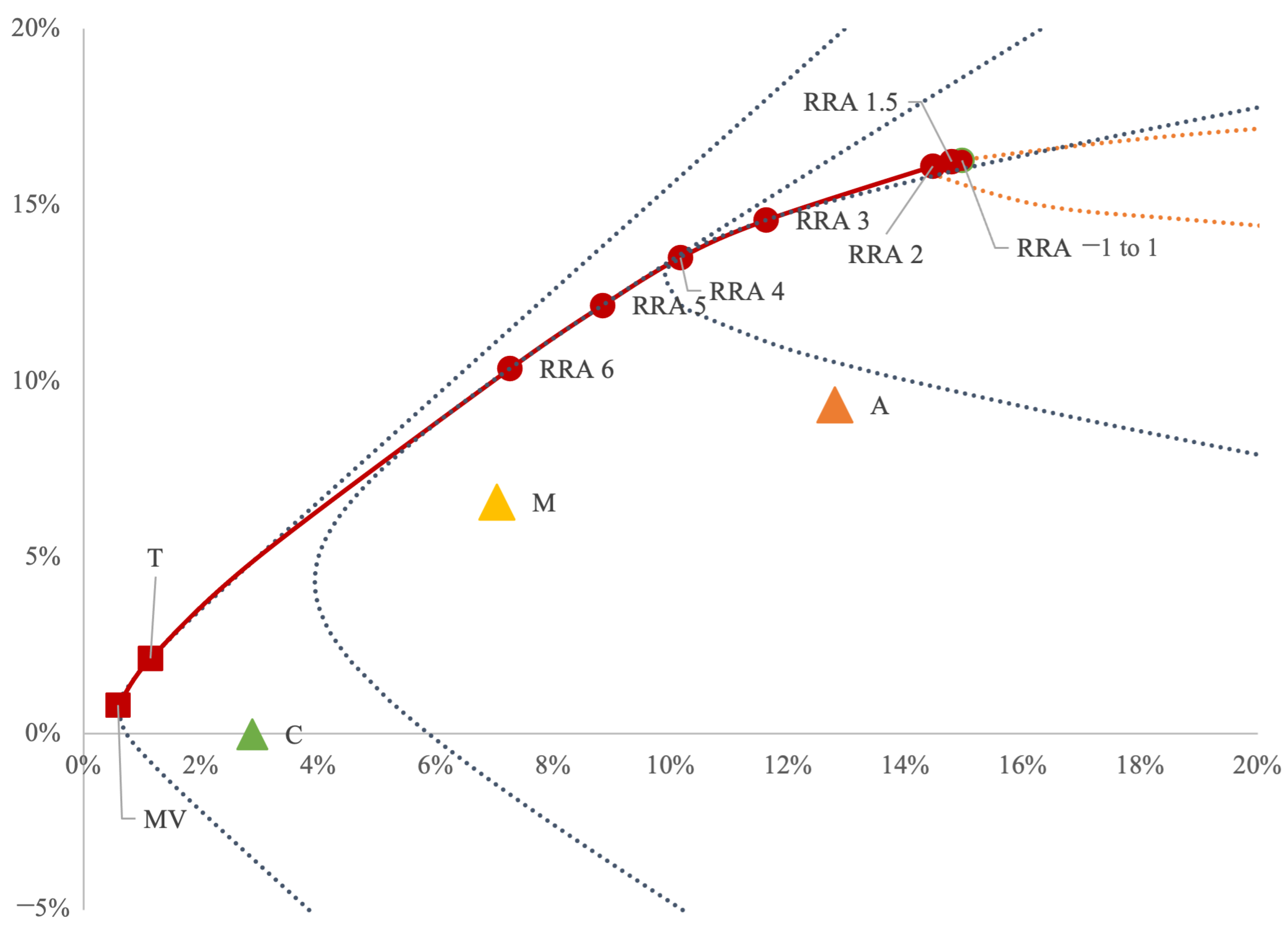
Figure 3 shows the (in-sample) mean-variance representation of all portfolios.

From Figure 3, it is evident that the robo portfolios, along with the naive homogeneous portfolio, fall within the historical efficient frontier (EF). This suggests that these portfolios were likely selected based on criteria other than mean-variance efficiency or that the inputs used by the robo advisor significantly deviated from historical data. The EF itself encompasses subsets of different hyperbolas, as expected in the case of no shortselling. This observation is further supported by the portfolio compositions outlined in Table 3, where the set of assets varies across different $RRA$ optimal portfolios.

When comparing the positions of the $RRA$-optimized portfolios with those recommended by the online platform, it becomes apparent that the Riskalyze conservative portfolio exhibits a significantly lower risk than all our $RRA$ portfolios. The moderate portfolio shows volatility comparable to the optimal portfolio when considering $RRA=6$, and the aggressive portfolio appears to align with an $RRA=3$. Assuming real-life levels of risk aversion to be less than three, as suggested by [33], we could assert that the robo advisor is ultraconservative, even with the most aggressive portfolio.

Table 2 and Table 3 and Figure 3 demonstrate that in-sample $RRA$ portfolios are more efficient. Consequently, it can be asserted that investors seeking efficient portfolios would be better off with $RRA$ portfolios than with robo portfolios. Up to now, we are looking in-sample, where the Riskalyze-proposed portfolios proved to be inefficient. However, it is crucial to acknowledge that in-sample comparisons may not present a comprehensive evaluation. The genuine challenge lies in assessing the out-of-sample performance of all portfolios.

4.2. Out-of-Sample

We aim to observe the actual/forward performance of the portfolios proposed based only on information up to 31 March 2017. As previously mentioned, the investment horizon of such portfolios is 5 years; thus, until the end of March 2022. Unfortunately, our out-of-sample finishes in March 2020 because of the COVID-19 pandemic, so this out-of-sample analysis relies only on the first 3 years of investment. Still, we find our out-of-sample results to be sound.

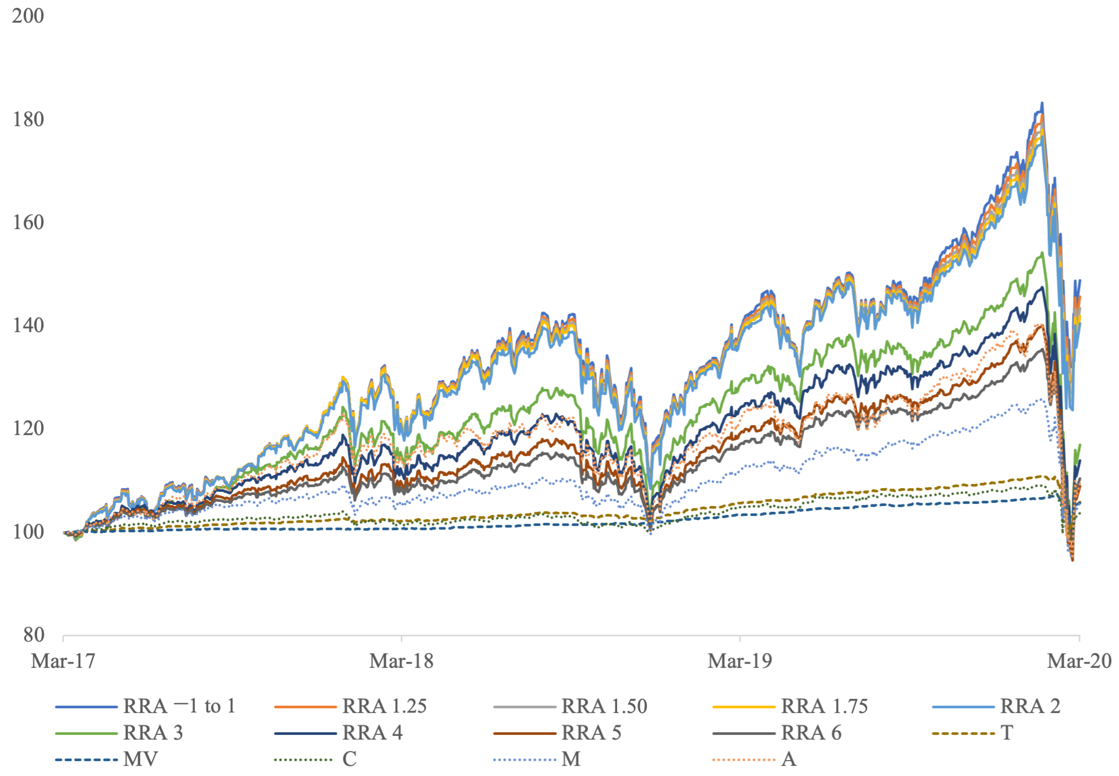
We consider a notional investment of USD 100 in each portfolio, and from there see how it evolves. We assume monthly rebalancing in order to realign the weightings of the portfolio. From Figure 4, we can see how the portfolios created by us evolved from 31 March 2017 to 31 March 2020.

Only by looking in terms of evolution, we see that the $RRA$ portfolios do considerably better than the other portfolios. The most aggressive ($RRA<2$) performed better, with the first strategy in terms of the final value being that of the risk lovers and risk-neutral. For levels of risk aversion between three and six, the performance gets close to that of the aggressive portfolio, A, of Riskalyze. The moderate portfolio of Riskalyze, M, performs below all the $RRA$ portfolios, but still higher than the worst three: the $MV$; T; and the conservative, C, Riskalyze portfolio.

The somewhat poor out-of-sample performance of the theoretical MVT portfolios, T and $MV$, is not unexpected due to the inherent estimation risk [36] of T and the reduced volatility of $MV$. Nevertheless, it is reassuring that $RRA$ portfolios exhibit greater robustness.

Table 4. Annual evolution of USD 100 investment.

Portfolio	29 March 2018	29 March 2019	30 March 2020
RRA −1.00–1.00	122.01	138.07	148.85
RRA 1.25	121.88	137.62	145.68
RRA 1.5	121.79	137.30	143.48
RRA 1.75	121.72	137.07	141.93
RRA 2	121.11	136.56	140.57
RRA 3	115.61	128.34	117.02
RRA 4	112.39	123.85	113.95
RRA 5	109.99	118.97	108.96
RRA 6	108.75	116.87	110.43
T	102.25	105.69	105.93
MV	100.74	103.43	105.70
H	109.14	113.76	104.62
C	101.89	104.96	103.71
M	106.04	111.82	105.77
A	114.77	121.19	109.61

presents the annual values of the USD 100 investment on the 3-year out-of-sample period. The most relevant results are, however, those in

Table 5. Out-of-sample performance of the various portfolios ranked by Sharpe ratio.

Portfolios	${\overline{\mathit{R}}}_{\mathit{p}}$	${\mathit{\sigma }}_{\mathit{p}}$	SR
MV	1.84%	0.03	0.8493
RRA −1.00–1.00	13.21%	0.23	0.5859
RRA 1.25	12.49%	0.23	0.5617
RRA 1.5	11.99%	0.23	0.5440
RRA 1.75	11.63%	0.23	0.5309
RRA 2	11.31%	0.22	0.5257
RRA 3	11.31%	0.22	0.5257
T	1.91%	0.05	0.4483
C	1.21%	0.05	0.3315
RRA 6	3.29%	0.14	0.2693
RRA 4	4.33%	0.18	0.2620
M	1.86%	0.12	0.1975
RRA 5	2.85%	0.17	0.1974
A	3.05%	0.19	0.1871
H	1.50%	0.13	0.1520

where the portfolios show up ranked—higher to lower—by Sharpe ratios. These ratios cover the investment over the entire 3 years of the out-of-sample data. Once again we see the $RRA$ portfolios performing reasonably well. We also note that, in general, the Sharpe ratios decrease when compared to the in-sample values.

In contrast to the observations in Table 2, the robo portfolio that, in Table 5, exhibits superior performance is the conservative C, followed by the moderate M and the aggressive A, contrary to economic intuition. The robo performance is primarily influenced by low volatility rather than returns. In contrast, $RRA$ portfolios showcase a performance driven by both returns and volatility, declining with an increase in the level of risk aversion, as one would anticipate.

Purely in terms of risk, and as in Figure 3, we continue to witness (now in Table 5) similar volatilities between A and $RRA3$ and M and $RRA6$ while C presents an extremely low volatility inconsistent with all levels of risk aversion considered. This supports the idea that robo portfolios may be ultraconservative for real-life investors.

5. Conclusions

The objective of this research is to introduce a methodology for robo advisors to integrate the risk profiles of individual investors into their portfolio construction. Our emphasis is on the analytical frameworks derived from mean-variance theory and expected utility theory, and we propose the construction of relative risk aversion ($RRA$) optimal portfolios.

We perform a comparative analysis between three portfolios generated by Riskalyze and those constructed by us. This comparison allowed us to conclude that their methodology does not “align” with ours.

In terms of performance, our results reveal that during the in-sample period, optimizing portfolios for varying levels of $RRA$ is more favorable than choosing portfolios provided by the Riskalyze platform. This preference is substantiated by our portfolios exhibiting a superior Sharpe Ratio, indicating an enhanced portfolio performance. Riskalyze portfolios do not seem to be mean-variance efficient (at least if we use historical MVT inputs). We also noted that the level of volatilities presented by the Riskalyze portfolios seems to be too low to be consistent with realistic levels of risk aversion ($RRA\le 3$).

Transitioning to the out-of-sample period, we confirm the good performance of the $RRA$ optimal portfolios. The Riskalyze portfolios show Sharpe ratios from 0.18 to 0.33 with the surprising result that it is the conservative portfolio presenting the highest value and the aggressive presenting the lowest, while $RRA$ portfolios with $RRA\le 3$ present Sharpe ratios from 0.52 to 0.58.

This analysis is, of course, not free of limitations. In particular, we use data only on three portfolios proposed by Riskalyze at a particular moment in time. Although interesting, one should be careful not to extrapolate these results to all Riskalyze portfolios and even more so not to extrapolate to other robo advisors. It would be interesting to look more systematically into real-life robo portfolios, but as mentioned, these are data that are simply not available. Also, just like most robos, we focus on individual investors. How to extend the proposed method to institutional investors is an open question.

But even if we focus only on individual investors, the usage of the $RRA$ method proposed here inherits the limitations of mean-variance theory (considering that investors only care about expected returns and variances) and expected utility theory (assuming enough rationality). Besides that, the measurement of RRA via investor questionnaires is sometimes nontrivial. A way to go around this last limitation is to consider a range of RRA values and analyze the portfolio composition’s evolution.

We hope this study contributes to a better understanding of robo advisors. Above all, we hope robos will start using more accurate methods of investor profiling, perhaps the method here proposed.

References

- Coffi, J.; George, B. The Fintech Revolution and the Changing Role of Financial Advisors. J. Appl. Theor. Soc. Sci. 2022, 4, 261–274. [Google Scholar] [CrossRef]
- Fisch, J.E.; Labouré, M.; Turner, J.A. The Emergence of the Robo-advisor. In The Disruptive Impact of FinTech on Retirement Systems; Agnew, J., Mitchell, O., Eds.; Oxford University Press Oxford: Oxford, UK, 2019; Chapter 2; pp. 13–37. [Google Scholar]
- Ben-David, D.; Sade, O. Robo-Advisor Adoption, Willingness to Pay, and Trust—Before and at the Outbreak of the COVID-19 Pandemic; SSRN Working Paper Series. 2001. Available online: https://www.semanticscholar.org/paper/Robo-Advisor-Adoption%2C-Willingness-to-Pay%2C-and-and-Ben-David-Sade/bdbc204c426e6ef74508ee8004715efeefa10bff (accessed on 1 October 2023).
- Tao, R.; Su, C.W.; Xiao, Y.; Dai, K.; Khalid, F. Robo advisors, algorithmic trading and investment management: Wonders of fourth industrial revolution in financial markets. Technol. Forecast. Soc. Chang. 2021, 163, 120421. [Google Scholar] [CrossRef]
- Tertilt, M.; Scholz, P. To advise, or not to advise—how robo-advisors evaluate the risk preferences of private investors. J. Wealth Manag. 2018, 21, 70–84. [Google Scholar] [CrossRef]
- Pedroni, A.; Frey, R.; Bruhin, A.; Dutilh, G.; Hertwig, R.; Rieskamp, J. The risk elicitation puzzle. Nat. Hum. Behav. 2017, 1, 803–809. [Google Scholar] [CrossRef] [PubMed]
- Gill, A.; Sinha, A.; Azim, F.; Silva, P.M.; Bernal, J. The Evolution of Robo-Advising; Technical Report; NYU Stern: New York, NY, USA, 2017. [Google Scholar]
- Acemoglu, D.; Restrepo, P. Robots and jobs: Evidence from US labor markets. J. Political Econ. 2020, 128, 2188–2244. [Google Scholar] [CrossRef]
- Deloitte. Executive Summary World Robotics 2019; Deloitte Technical Report; Deloitte: Brussels, Belgium, 2019. [Google Scholar]
- Al Nawayseh, M.K. Fintech in COVID-19 and beyond: What factors are affecting customers’ choice of fintech applications? J. Open Innov. Technol. Mark. Complex. 2020, 6, 153. [Google Scholar] [CrossRef]
- Phoon, K.; Koh, F. Robo-advisors and wealth management. J. Altern. Investig. 2017, 20, 79–94. [Google Scholar] [CrossRef]
- D’Acunto, F.; Prabhala, N.; Rossi, A.G. The promises and pitfalls of robo-advising. Rev. Financ. Stud. 2019, 32, 1983–2020. [Google Scholar] [CrossRef]
- Back, C.; Morana, S.; Spann, M. When do robo-advisors make us better investors? The impact of social design elements on investor behavior. J. Behav. Exp. Econ. 2023, 103, 101984. [Google Scholar] [CrossRef]
- Bhatia, A.; Chandani, A.; Divekar, R.; Mehta, M.; Vijay, N. Digital innovation in wealth management landscape: The moderating role of robo advisors in behavioural biases and investment decision-making. Int. J. Innov. Sci. 2022, 14, 693–712. [Google Scholar] [CrossRef]
- Brenner, L.; Meyll, T. Robo-advisors: A substitute for human financial advice? J. Behav. Exp. Financ. 2020, 25, 100275. [Google Scholar] [CrossRef]
- Gaspar, R.M.; Henriques, P.L.; Corrente, A.R. Trust in financial markets: The role of the human element. Rev. Bras. Gest. Negocios 2020, 22, 647–668. [Google Scholar] [CrossRef]
- Macchiavello, E.; Siri, M. Sustainable Finance and Fintech: Can Technology Contribute to Achieving Environmental Goals? A Preliminary Assessment of ‘Green Fintech’and ‘Sustainable Digital Finance’. Eur. Financ. Law Rev. 2022, 19, 128–174. [Google Scholar] [CrossRef]
- Maume, P. Robo-Advisors: How Do They Fit in the Existing EU Regulatory Framework, in Particular with Regard to Investor Protection?: Study Requested by the ECON Committee; European Parliament technical Report: Luxembourg, 2021.
- Boreiko, D.; Massarotti, F. How risk profiles of investors affect robo-advised portfolios. Front. Artif. Intell. 2020, 3, 60. [Google Scholar] [CrossRef] [PubMed]
- Jung, D.; Dorner, V.; Glaser, F.; Morana, S. Robo-advisory: Digitalization and automation of financial advisory. Bus. Inf. Syst. Eng. 2018, 60, 81–86. [Google Scholar] [CrossRef]
- Méndez-Suárez, M.; García-Fernández, F.; Gallardo, F. Artificial intelligence modelling framework for financial automated advising in the copper market. J. Open Innov. Technol. Mark. Complex. 2019, 5, 81. [Google Scholar] [CrossRef]
- Baek, S.; Lee, K.Y.; Uctum, M.; Oh, S.H. Robo-Advisors: Machine Learning in Trend-Following ETF Investments. Sustainability 2020, 12, 6399. [Google Scholar] [CrossRef]
- Perrin, S.; Roncalli, T. Machine learning optimization algorithms & portfolio allocation. In Machine Learning for Asset Management: New Developments and Financial Applications; John Wiley & Sons: London, UK, 2020; pp. 261–328. [Google Scholar]
- Anshari, M.; Almunawar, M.N.; Masri, M. Digital twin: Financial technology’s next frontier of robo-advisor. J. Risk Financ. Manag. 2022, 15, 163. [Google Scholar] [CrossRef]
- Neumann, J.v.; Morgenstern, O. Theory of Games and Economic Behavior; Princeton University Press Princeton: Princeton, NJ, USA, 1947. [Google Scholar]
- Gai, P.; Vause, N. Measuring Investors’ Risk Appetite; Bank of England Working Paper Series. Available online: https://www.ecb.europa.eu/pub/pdf/fsr/art/ecb.fsrart200706_04.en.pdf (accessed on 1 October 2023).
- Hanna, S.D.; Gutter, M.S.; Fan, J.X. A measure of risk tolerance based on economic theory. J. Financ. Couns. Plan. 2001, 12, 53. [Google Scholar]
- Alsabah, H.; Capponi, A.; Ruiz Lacedelli, O.; Stern, M. Robo-advising: Learning investors’ risk preferences via portfolio choices. J. Financ. Econom. 2021, 19, 369–392. [Google Scholar] [CrossRef]
- Capponi, A.; Olafsson, S.; Zariphopoulou, T. Personalized robo-advising: Enhancing investment through client interaction. Manag. Sci. 2022, 68, 2485–2512. [Google Scholar] [CrossRef]
- Firmansyah, E.A.; Masri, M.; Anshari, M.; Besar, M.H.A. Factors affecting fintech adoption: A systematic literature review. FinTech 2022, 2, 21–33. [Google Scholar] [CrossRef]
- Suryono, R.R.; Budi, I.; Purwandari, B. Challenges and trends of financial technology (Fintech): A systematic literature review. Information 2020, 11, 590. [Google Scholar] [CrossRef]
- Lam, J.W. Robo-Advisors: A Portfolio Management Perspective. Master’s Thesis, Yale College, New Haven, CT, USA, 2016. [Google Scholar]
- Meyer, D.J.; Meyer, J. Relative risk aversion: What do we know? J. Risk Uncertain. 2005, 31, 243–262. [Google Scholar] [CrossRef]
- Almadi, H.; Rapach, D.E.; Suri, A. Return predictability and dynamic asset allocation: How often should investors rebalance? J. Portf. Manag. 2014, 40, 16–27. [Google Scholar] [CrossRef]
- Zakamouline, V.; Koekebakker, S. Portfolio performance evaluation with generalized Sharpe ratios: Beyond the mean and variance. J. Bank. Financ. 2009, 33, 1242–1254. [Google Scholar] [CrossRef]
- Cardoso, J.; Gaspar, R. Estimation risk and robust mean variance. In Mean-Variance Theory Mean-Variance Theory: Applications and Risks; Gaspar, R., Ed.; AEdition: Lisbon, Portugal, 2018; Chapter 4; pp. 95–120. [Google Scholar]