NeuroAdaptiveNet: A Reconfigurable FPGA-Based Neural Network System with Dynamic Model Selection

Abstract

This paper presents NeuroAdaptiveNet, an FPGA-based neural network framework that dynamically self-adjusts its architectural configurations in real time to maximize performance across diverse datasets. The core innovation is a Dynamic Classifier Selection mechanism, which harnesses the k-Nearest Centroid algorithm to identify the most competent neural network model for each incoming data sample. By adaptively selecting the most suitable model configuration, NeuroAdaptiveNet achieves significantly improved classification accuracy and optimized resource usage compared to conventional, statically configured neural networks. Experimental results on four datasets demonstrate that NeuroAdaptiveNet can reduce FPGA resource utilization by as much as 52.85%, increase classification accuracy by 4.31%, and lower power consumption by up to 24.5%. These gains illustrate the clear advantage of real-time, per-input reconfiguration over static designs. These advantages are particularly crucial for edge computing and embedded applications, where computational constraints and energy efficiency are paramount. The ability of NeuroAdaptiveNet to tailor its neural network parameters and architecture on a per-input basis paves the way for more efficient and accurate AI solutions in resource-constrained environments.

1. Introduction

Neural networks [1] have emerged as a central pillar of machine learning [2], capable of detecting nuanced patterns in complex, large-scale datasets by emulating certain structural and functional characteristics of the human brain. Constructed from interconnected computational elements analogous to biological neurons, these networks excel in processing and relaying information across multiple layers. Crucially, the depth, configuration, and number of these layers significantly influence a network’s capacity to generalize and perform effectively in myriad real-world tasks.

This remarkable flexibility and performance have positioned neural networks as indispensable tools in diverse fields, including autonomous vehicles [3], healthcare [4], robotics [5], and telecommunications [6]. Despite their extensive applicability, deploying neural networks on resource-constrained platforms remains a formidable challenge, largely due to their high computational and memory requirements. These limitations can hinder their efficiency and broad adoption, particularly when rapid inference or low power consumption is demanded.

In addressing these computational constraints, researchers have increasingly focused on reconfigurable architectures [7], which offer a compelling balance between adaptability and performance. By enabling post-manufacturing modifications, reconfigurable systems provide hardware-level flexibility akin to that of software environments, allowing design parameters such as throughput, latency, and resource utilization to be fine-tuned to specific application demands. This adaptability is particularly well-suited for optimizing the performance of neural networks while minimizing hardware overhead.

Recent efforts to implement neural networks on Field-Programmable Gate Arrays (FPGAs) highlight the promise of reconfigurable solutions. For instance, [8] introduces a pragmatic method for shrinking hardware-based neural networks by employing adaptable layers in Artificial Neural Networks, wherein each layer can execute two distinct functions. This approach achieves a remarkable 41% reduction in the FPGA footprint compared with alternative designs and demonstrates a straightforward, Verilog-based implementation on the Altera Arria 10 GX FPGA. Concurrently, ref. [9] proposes an adaptive parallelism strategy for Binary Neural Networks (BNNs) on a Xilinx XCZU7EV FPGA, thereby streamlining resource usage while preserving high throughput across varying BNN layers. This dynamic allocation of computational parallelism enables a substantial improvement in area–speed efficiency relative to previous FPGAs and VLSI accelerators, which is especially pertinent for real-time inference on edge devices.

Along similar lines, ref. [10] demonstrated a fully reconfigurable multilayer perceptron on a Cyclone IV FPGA that supports run-time adjustment of key network parameters, including number of inputs, neurons per layer, total layers, bias inclusion, and choice of activation function, entirely without re-synthesis. Their architecture reuses a fixed bank of 20 hardware neurons as virtual layers under the control of a finite-state machine, and replaces vendor-specific DSP blocks with custom VEDIC multipliers to ensure portability to ASIC implementations. Although the design operates at a lower peak clock rate (approximately 77 MHz), it achieves competitive performance, achieving 99.3% accuracy on the Iris classification task in 1.16 µs and sub-microsecond latency on function approximation, while consuming only 37% of logic elements and 1% of memory bits on the FPGA.

Prior FPGA-based accelerators have typically optimized only one or two metrics. For example, ref. [8] achieved a 41% reduction in footprint, ref. [9] reported a 24% improvement in area–speed efficiency, and [10] enabled per-task reconfiguration. In contrast, NeuroAdaptiveNet employs per-input reconfiguration to achieve simultaneous improvements in power consumption, hardware resource utilization, and classification accuracy.

At runtime, NeuroAdaptiveNet evaluates each input and switches to the most suitable compact neural model, resulting in up to 24.5% lower power consumption, up to 52.85% lower resource utilization, and up to 4.31% higher classification accuracy compared with the best static design. Unlike prior designs that use a fixed single network or adapt only at the task level, NeuroAdaptiveNet’s input-level flexibility incurs only microseconds of overhead while delivering maximum accuracy with minimal hardware and energy requirements. Its efficient performance and high accuracy make it an ideal solution for Edge AI systems constrained by limited power and resources. The primary goal of this study is to introduce a novel FPGA-based neural network implementation that departs from the conventional static design.

The remainder of this paper is structured as follows. Section 2 details the dynamic classifier selection framework, Section 3 explains the FPGA design, Section 4 reports accuracy, resource-use, power, and latency results, Section 5 analyzes trade-offs and future work, and Section 6 concludes the paper.

2. Dynamic Classifier Selection Mechanism

2.1. Background

Dynamic classifier selection (DCS) [11,12,13] is a specialized machine learning technique that, for each incoming data instance, selects the single most appropriate classifier from a larger ensemble of candidates. Unlike traditional methods relying on a fixed, one-size-fits-all model, DCS adaptively evaluates multiple classifiers in real time, choosing the one best suited to handle the current data point. Typically, the selection process gauges each classifier’s competence based on past performance metrics, similarity to the query instance, or a combination of such factors. By leveraging the diverse strengths of different classifiers, DCS enhances the overall accuracy and adaptability of the system—particularly in scenarios with highly variable data distributions or stringent accuracy requirements.

In our work, we employ a clustering-based framework for DCS, diverging from the widely used k-nearest neighbors (k-NN) method. Specifically, we implement the k-Nearest Centroid (k-NC) technique, building upon our earlier research with heterogeneous classifier ensembles [14] and a k-NN accelerator [15]. Here, however, we apply k-NC to a homogeneous set of neural network classifiers, each configured with different hyperparameters, while retaining the underlying insights from our hardware-centric ensemble research. A key advancement in this approach is its flexibility regarding the number of clusters, rather than directly coupling the number of centroids to the number of classes. This design choice facilitates more precise grouping of similar data points, thus improving competence estimation across varying data regions.

To realize this implementation, we pre-compute the centroids via the k-means algorithm (using Python’s scikit-learn library) and store them in a dedicated memory file for subsequent FPGA-based execution. We then evaluate all neural network configurations on each cluster within Python, thereby mapping each centroid to the network model that consistently delivers the highest accuracy for that cluster. As illustrated in Figure 1, this results in a refined selection mechanism wherein each cluster is paired with the top-performing classifier, yielding both improved accuracy and streamlined hardware utilization.

Upon receiving new test data, the system swiftly assigns it to the closest cluster, subsequently engaging the preselected, most efficient neural network model for that cluster’s classification task.

2.2. Methodology

In this methodology, we improve the diversity of the classifier by splitting the training dataset into two distinct subsets. The first subset is used to train the first half of our neural network models, while the second subset trains the remaining models. By doing so, each group of neural network configurations is exposed to different data patterns, thereby increasing the overall variety of learned representations and boosting the collective predictive accuracy.

Once a configuration is selected, its corresponding parameters (weights and biases) are applied to the base neural network, which is depicted in Figure 2 as a densely connected network of neurons. Around this core structure, multiple configurations, designated as Configuration 1 through Configuration x, offer alternative architectures by varying the number of neurons and other settings. Critically, when choosing which model to deploy, the system also loads the relevant weights and biases for that specific configuration, ensuring optimal alignment between the chosen architecture and its parameters. The DNN Configuration Selector oversees this dynamic selection process, applying the most suitable configuration to each incoming data sample for efficient, high-accuracy inference.

Figure 2 illustrates the operational flow of our adaptive neural network design. First, the input data are directed to the DNN Configuration Selector, which identifies the optimal configuration, designated Configuration x, for that particular data instance. The parameters of the selected configuration are then loaded into the base neural network, represented by a dense network of interconnected neurons. Each configuration (from Configuration 1 through Configuration x) reflects a possible adaptation of the base network, featuring different neuron counts and other hyperparameters. Crucially, selecting the corresponding weights and biases ensures that the chosen network is precisely tuned to the incoming data. This adaptive selection mechanism maximizes accuracy while maintaining operational efficiency, as each input is processed using the most appropriate model variant.

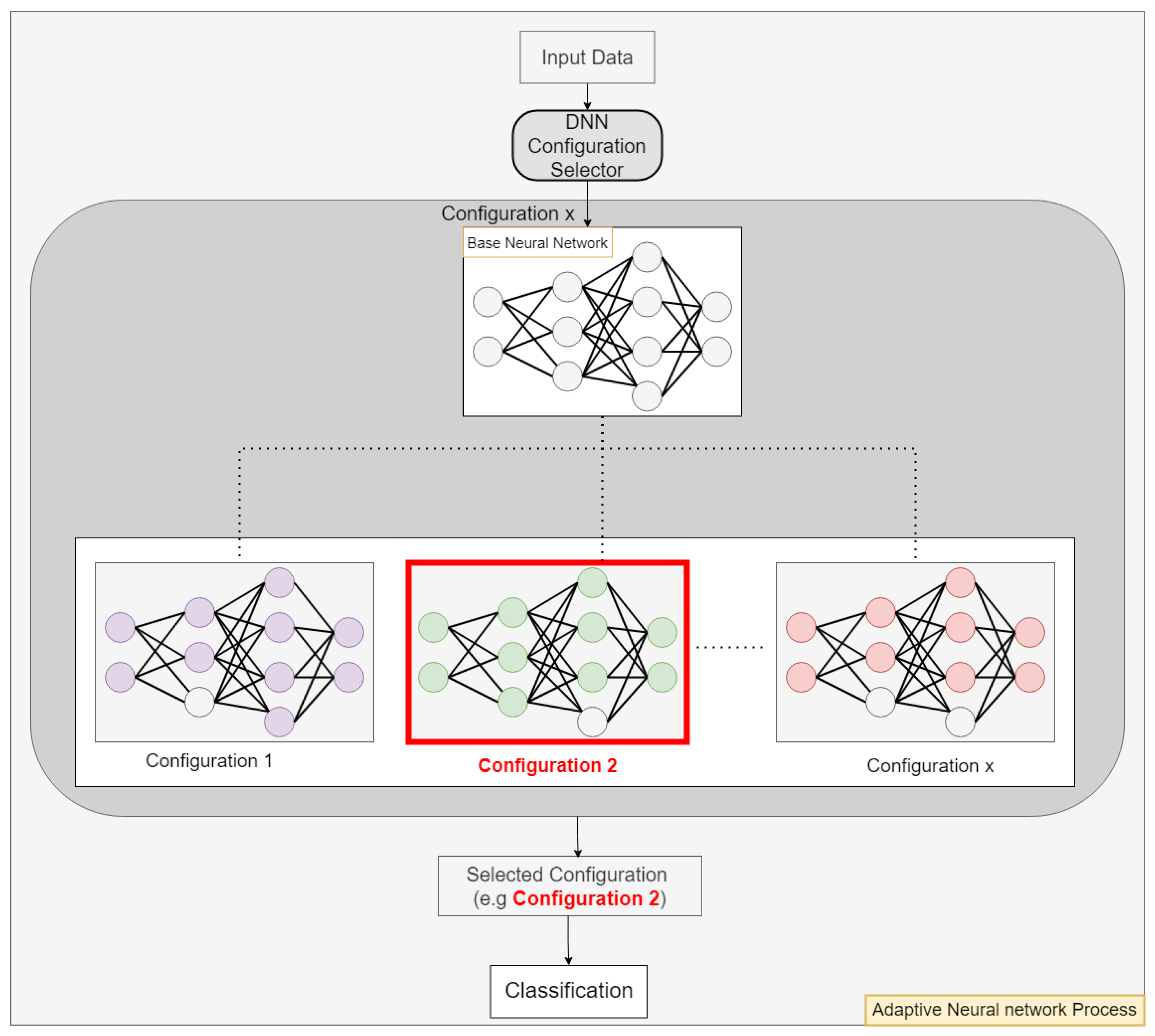
3. NeuroAdaptiveNet Design

We implemented the design using Verilog, creating two primary modules as depicted in Figure 3: the DNN Configuration Selector module and the DNN Accelerator module.

The DNN Configuration Selector module incorporates a Squared Euclidean Distance Unit that efficiently computes the distances between the input data vector and pre-stored centroids as shown in Figure 4. This computation is achieved through a pipeline of parallel subtractors, multipliers, and an accumulator.

Initially, parallel subtractors calculate the differences between each feature of the input vector and the corresponding features of a centroid. These differences are then squared by the multipliers and the resulting squared values are aggregated by the accumulator to yield the squared Euclidean distance for the centroid. The computation adheres to the formula shown in Equation (1), enabling precise distance measurement while optimizing hardware performance.

$$d(x,C)=\sqrt{\sum _{i=1}^n{(x_i-C_i)}^2}$$

(1)

where $x_i$ and $C_i$ are the individual features of the input vector and centroid.

After completing the centroid evaluations, the computed distances are temporarily stored in a buffer. A comparator examines these distances, identifies the smallest value, and retrieves its corresponding label to determine the most suitable neural network configuration. This selection process is facilitated by a lookup table, represented as the “configurations” block in Figure 3, which maps each closest centroid to its optimal neural network model configuration. This association ensures that each input data point is processed by the configuration best suited for accurate classification.

The Control Unit serves as a critical component, managing the data flow and overseeing all computational tasks within the system. It directs the neural network module to deploy the specific configuration identified by the DNN Configuration Selector, ensuring smooth operation and accurate classification.

In our FPGA architecture, each processing element mimics the function of a traditional neuron by carrying out Multiply-Accumulate operations followed by ReLU activation. Each processing element multiplies input vector elements $x_i$ by their corresponding weights W and adds a bias term b. This is mathematically represented as follows:

The implementation of the ReLU activation function is achieved using a comparator along with a 2:1 Multiplexer. This setup allows the activation function to be expressed mathematically as follows:

$$y=max(0,s)$$

(2)

This implementation allows each processing element to efficiently handle all necessary calculations and activation steps, closely mimicking the behavior of neurons in traditional neural network models. The architecture accommodates variable neuron counts and supports multiple layers. In a static implementation, the design instantiates as many processing elements as the size of the largest hidden layer. For NeuroAdaptiveNet, we instantiate processing elements equal to the maximum hidden-layer size across all configurations in the ensemble. This arrangement ensures that all neurons within each layer execute in parallel, while layers are processed sequentially.

In the output stage, the commonly used softmax activation is replaced by the argmax function to better align with our focus on maximizing classification accuracy. The argmax function identifies the neuron with the highest output and converts this information into a one-hot encoded vector, circumventing the need for complete class probability distributions. This streamlined approach reduces computational overhead, simplifies hardware complexity, and accelerates inference.

4. Results

4.1. Dataset and Pre-Processing

We evaluate the NeuroAdaptiveNet system, implemented on an FPGA, using four distinct datasets from the UCI repository: Pima Indian Diabetes, Vehicle Silhouettes, Connect-4, and German Credit. These datasets vary in complexity and classification tasks, with Pima Indian Diabetes and German Credit tailored for binary classification and Vehicle Silhouettes and Connect-4 involving multiclass classification.

To maintain uniformity across these heterogeneous datasets, we adopt an 85–15 split for data partitioning. Specifically, 85% of each dataset is used both to train the models and to compute centroids. The remaining 15% of the data is held out for testing and performance evaluation, enabling a comprehensive assessment of the system’s accuracy and robustness.

The design is implemented on an Ultra96v2 board featuring the Zynq UltraScale+ MPSoC. Our FPGA implementations employ a 16-bit fixed-point format for all input vectors, weights, biases, and centroids.

We run scikit-learn’s KMeans multiple times to generate different centroid initializations, then select the initialization that performs best on a validation subset of the training data.

4.2. Configurations

We employ a small ensemble of compact neural networks that differ in both their training data and their architecture. To create this ensemble, we partition the full training set into two subsets and train half of our network configurations on the first subset and the other half on the second. Each configuration also varies the number of neurons per layer. Although this ensemble is not intended to represent the optimal combination of models, it demonstrates that selecting from a diverse collection of smaller networks for each individual input can achieve a more resource and energy-efficient adaptive implementation than relying on a single, statically configured network.

Table 1. Neural network configuration parameters.

NN Configurations	Lj (Vehicle)	Lj (Diabetes)	Lj (German Credit)	Lj (Connect-4)
Base-NN	(22, 22, 16)	(6, 6)	(8, 8)	(30, 30, 22)
NN1	(22, 22, 12)	(6, 6)	(7, 7)	(30, 30, 20)
NN2	(18, 18, 10)	(4, 4)	(5, 5)	(29, 29, 22)
NN3	(18, 18, 14)	(3, 3)	(4, 4)	(30, 30, 22)
NN4	(20, 20, 15)	(4, 4)	(6, 4)	(29, 29, 21)
NN5	(20, 20, 16)	(5, 3)	(6, 6)	(27, 27, 20)
NN6	N/A	N/A	(8, 8)	(30, 30, 18)
NN7	N/A	N/A	N/A	(28, 28, 20)

lists the network configurations that make up the NeuroAdaptiveNet ensemble for each dataset. Each configuration is defined by its layer-wise neuron counts, ensuring a diverse set of model. At runtime, the DNN Configuration Selector chooses the configuration best suited to the current input and the accelerator dynamically loads its corresponding weights, biases, and neuron-count settings before performing inference.

Upon receiving an input sample, the selector identifies the optimal network configuration, which is defined by its layer-wise neuron counts, weight matrices, and bias vectors. The accelerator then loads these parameters and performs inference by processing exactly the specified neurons in each layer. We train each network configuration in Python 3.8 and export its weights and bias vectors into memory initialization files.

4.3. Accuracy Results

With the ensemble configurations defined, we now evaluate the classification accuracy of NeuroAdaptiveNet against static network designs.

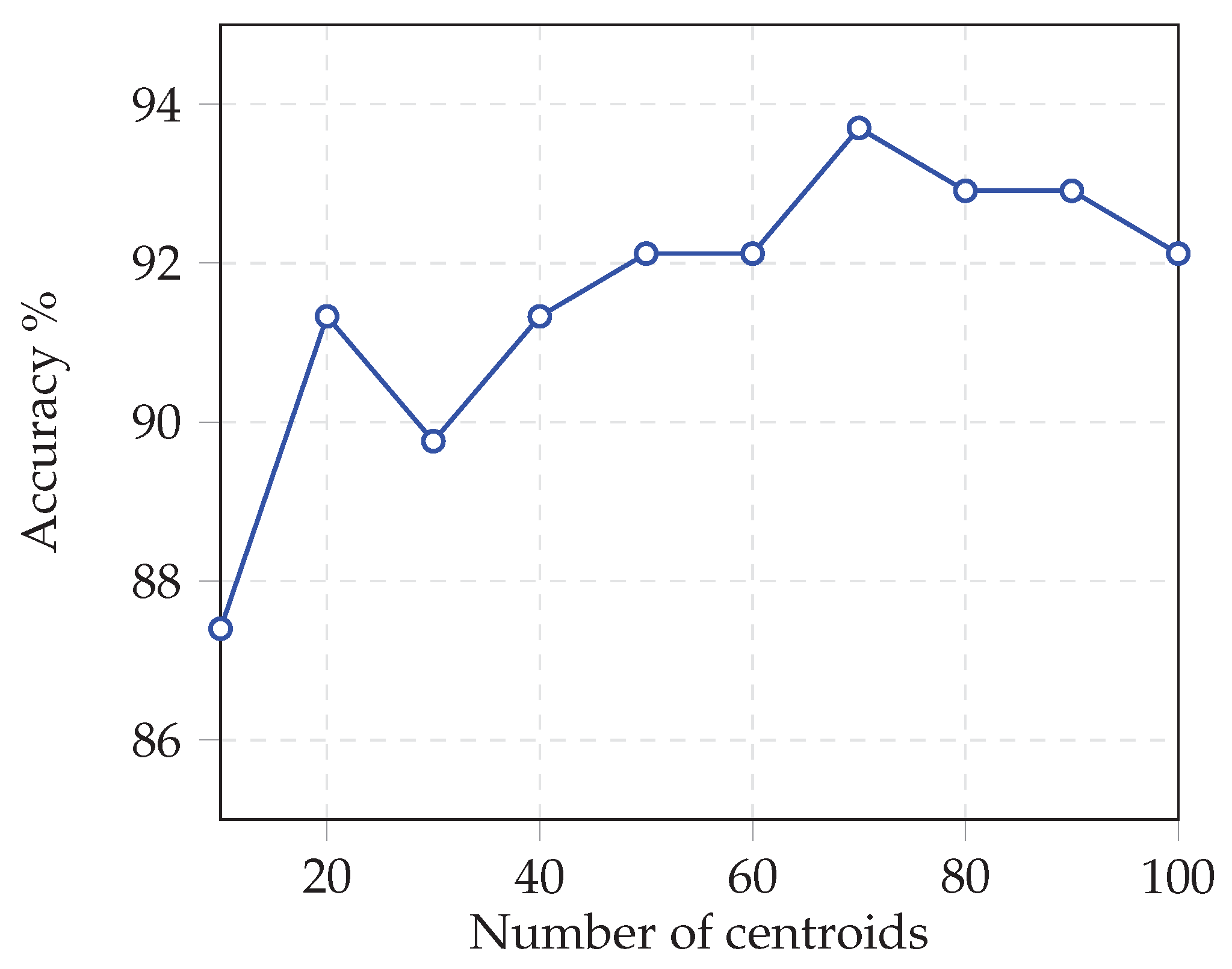
Determining the optimal number of centroids C is critical. This parameter has a critical impact on accuracy. To identify the best value, we ran a series of experiments varying the number of centroids from 10 to 100 for smaller datasets and from 10 to 200 for larger ones. Figure 5 shows how accuracy on the Vehicle dataset improves as the number of centroids increases.

Figure 5 clearly shows that increasing the number of centroids from 10 to 70 raises classification accuracy from 87.40% to 93.70%. This improvement occurs because each additional centroid refines the partitioning of the feature space, creating more regions in which a specialized network can operate.

Following comprehensive experiments to determine each dataset’s optimal centroid count, we evaluate NeuroAdaptiveNet performance against static neural network models with larger, denser architectures, as shown in

Table 2. Neural network model accuracy comparison.

Dataset	NeuroAdaptive Net	Larger NN Implementations (Hidden Layers/Accuracy)	Performance Difference
Vehicle	93.70%	(40, 40, 20)/89.76%	3.94%
		(60, 60, 30)/91.33%	2.37%
Diabetes	87.93%	(16, 16)/83.62%	4.31%
German	85.33%	(32, 32)/81.33%	4.00%
Connect-4	80.24%	(60, 60, 30)/79.85%	0.39%
		(90, 90, 60)/79.81%	0.43%
		(120, 120, 64)/80.05%	0.19%

.

The results indicate that the NeuroAdaptiveNet system outperforms the traditional models in all tested datasets, achieving up to 4.31% more accuracy. The NeuroAdaptiveNet showed higher accuracy compared to several larger networks employing the standard approach. This pattern of enhanced performance was consistent across all datasets, with the NeuroAdaptiveNet system demonstrating a clear advantage over the traditional setups.

For the Vehicle Silhouettes and German Credit datasets, the best configuration was achieved with 70 centroids. In contrast, the Diabetes dataset reached optimal performance with a different centroid count of 50, while the Connect-4 dataset required 180 centroids for the best results.

4.4. Resource Utilization and Power Analysis

Resource usage is a key indicator of FPGA designs efficiency. In this analysis, we compare how much hardware different neural network models use for all datasets. This helps us understand which designs are most efficient for specific applications.

Across all four benchmarks, as shown in

Table 3. Resource utilization comparison for Vehicle dataset.

Resource	(60, 60, 30)	NeuroAdaptiveNet	Resource Decrease (%)
LUT	9655	8860	8.23
FF	6238	3995	35.96
DSP	128	73	42.97

,

Table 4. Resource utilization comparison for Connect-4 dataset.

Resource	(120, 120, 64)	NeuroAdaptiveNet	Resource Decrease (%)
LUT	22,261	19,032	14.51
FF	11,633	5706	50.95
DSP	246	116	52.85

,

Table 5. Resource utilization comparison for Diabetes dataset.

Resource	(16, 16)	NeuroAdaptiveNet	Resource Decrease (%)
LUT	2122	1914	9.80
FF	1944	1567	19.39
DSP	36	27	25.00

and

Table 6. Resource utilization comparison for German-Credit dataset.

Resource	(32, 32)	NeuroAdaptiveNet	Resource Decrease (%)
LUT	8988	8636	3.92
FF	6774	4418	34.78
DSP	128	77	39.84

, NeuroAdaptiveNet delivers consistent FPGA resource savings: LUT utilization decreases by roughly 4% to 15%, FF usage by approximately 19% to 51%, and DSP consumption by about 25% to 53%. These results demonstrate that NeuroAdaptiveNet effectively minimizes hardware utilization without sacrificing accuracy. These resource reductions result from NeuroAdaptiveNet’s dynamic use of compact networks, each of which requires fewer processing elements than a single, larger fixed design.

We observed that NeuroAdaptiveNet uses more LUTRAM than a single static design. This increase results from storing multiple parameter sets, including each configuration’s weights and biases, as well as the centroid feature vectors required by the DNN Configuration Selector.

To assess the energy efficiency of our adaptive architecture, we performed post-implementation power estimation in Xilinx Vivado, targeting the programmable logic of an Ultra96-V2 board (Zynq UltraScale+ MPSoC). NeuroAdaptiveNet was configured with the centroid counts that maximize classification accuracy for each dataset, and its PL dynamic power consumption was compared against the highest-performing static Neural network implementation. The results are summarized in

Table 7. Dynamic PL power consumption and percentage decrease.

Dataset	Configuration	Power (W)	Decrease (%)
Connect	NeuroAdaptiveNet (C = 180)	1.036	10.1
	(120, 120, 64)	1.152
Diabetes	NeuroAdaptiveNet (C = 50)	0.154	24.5
	(16, 16)	0.204
Vehicle	NeuroAdaptiveNet (C = 70)	0.591	1.5
	(60, 60, 30)	0.600
German	NeuroAdaptiveNet (C = 70)	0.220	18.2
	(32, 32)	0.269

.

Table 7 presents the dynamic PL power consumption of NeuroAdaptiveNet when configured with the centroid counts (C) that yielded the highest classification accuracy on each dataset, compared against the corresponding neural networks (120, 120, 64) for Connect-4, (16, 16) for Diabetes, (60, 60, 30) for Vehicle, and (32, 32) for German-Credit, NeuroAdaptiveNet achieves power savings of 10.1%, 24.5%, 1.5%, and 18.2%, respectively. These findings confirm that NeuroAdaptiveNet consistently reduces FPGA power consumption compared to conventional fixed neural networks, achieving substantial energy savings without sacrificing accuracy.

4.5. Latency Analysis

Inference latency is a key metric for real-time neural network applications.

Table 8. Maximum frequency and inference latency.

Dataset	Configuration	${\mathit{F}}_{\mathbf{max}}$ (MHz)	Latency (μs)
Connect	C = 180	301.11	1.76
	(120, 120, 64)	308.54	1.09
Diabetes	C = 50	311.72	0.49
	(16, 16)	325.20	0.17
Vehicle	C = 70	314.96	0.83
	(60, 60, 30)	305.43	0.60
German	C = 70	322.26	0.67
	(32, 32)	321.13	0.27

presents the measured maximum clock frequencies and inference latencies for NeuroAdaptiveNet.

The integration of the DNN Configuration Selector for centroid evaluation adds only a small latency overhead. Inference latency increases by 0.67 µs on Connect-4, 0.32 µs on Diabetes, 0.23 µs on Vehicle, and 0.40 µs on German-Credit.

5. Discussion

The NeuroAdaptiveNet framework, optimized for FPGA deployment, delivers remarkable hardware efficiency and classification accuracy. It relies on a k-nearest centroid mechanism, a distance-based approach akin to k-NN, making it susceptible to the curse of dimensionality [16]. As feature dimensionality increases, the number of subtractors, multipliers, and accumulators required to compute distances grows substantially, and the memory must store larger centroid vectors. The increased computational and storage requirements can offset the advantages of the method when applied to very high-dimensional data. To enhance its performance, dimensionality reduction techniques such as principal component analysis (PCA) or neural autoencoders can be employed to compress high-dimensional features into more compact, informative representations [17]. Additionally, designing adaptive distance metrics tailored for high-dimensional spaces can refine feature comparisons and reduce computational complexity. These additional improvements could potentially preserve the efficiency of NeuroAdaptiveNet while extending its applicability to real-time FPGA-based systems that manage complex, large-scale datasets.

6. Conclusions

The NeuroAdaptiveNet system represents a novel approach to FPGA-based neural networks, offering dynamic adaptability and high accuracy for real-time and edge computing scenarios. Experimental results across diverse datasets confirm its effectiveness in adjusting neural network configurations on a per-input basis, thus balancing hardware resource management and classification performance.

By capitalizing on an adaptive architecture that reconfigures its parameters in response to incoming data, NeuroAdaptiveNet showcases significant benefits over static neural network models, particularly in terms of efficiency and response time. This ability to select the most suitable neural configuration for each input greatly enhances its applicability in resource-limited environments where computational demands and power constraints are paramount.

Looking ahead, the integration of dimensionality reduction techniques and specialized distance metrics offers promising avenues to counteract the limitations posed by high-dimensional data. These enhancements have the potential to reinforce the adaptability of NeuroAdaptiveNet, further increasing its performance in a wide range of real-time and edge computing applications. Ultimately, the system’s flexibility and efficiency mark a meaningful step forward in developing next-generation, FPGA-optimized neural network solutions.