Advances in Unsupervised Parameterization of the Seasonal–Diurnal Surface Wind Vector

Abstract

The Offset Elliptical Normal (OEN) mixture model represents the seasonal–diurnal surface wind vector for wind engineering design applications. This study upgrades the parameterization of OEN by accounting for changes in format of the global database of surface observations, improving performance by eliminating manual supervision and extending the scope of the model to include skewness. The previous coordinate transformation of binned speed and direction, used to evaluate the joint probability distributions of the wind vector, is replaced by direct kernel density estimation. The slow process of sequentially adding additional components is replaced by initializing all components together using fuzzy clustering. The supervised process of sequencing each mixture component through time is replaced by a fully automated unsupervised process using pattern matching. Previously reported departures from normal in the tails of the fuzzy-demodulated OEN orthogonal vectors are investigated by directly fitting the bivariate skew generalized t distribution, showing that the small observed skew is likely real but that the observed kurtosis is an artefact of the demodulation process, leading to a new Offset Skew Normal mixture model. The supplied open-source R scripts fully automate parametrization for locations in the NCEI Integrated Surface Hourly global database of wind observations.

1. Introduction

The seasonal and diurnal variation of the wind speed vector is an important consideration in many engineering applications and is almost universally represented statistically by the probability of occurrence. Applications include the assessment of wind energy potential, the design and operation of wind-sensitive structures, the specification of heating and ventilation systems, pollution dispersal studies and the assessment of pedestrian safety and comfort in urban areas. These statistical models are also the essential first step in codes and regulations for the design of buildings to resist wind loads.

The observed seasonal–diurnal variation of the wind vector presents as annual and daily cycles with random perturbations. The Offset Elliptical Normal (OEN) mixture model, developed over the last decade [1,2,3,4], represents these perturbations as elliptical bivariate normal distributions in the zonal–meridional plane with their centers offset from the origin by the annual and daily cycles of the mean vector. This model is founded on the physical/statistical theory for upper-air winds proposed in 1946 by Brooks and Carruthers [5] and later developed by Crutcher et al. [6,7,8,9]. Its applicability to surface winds [1] relies on no relevant constraints on the wind vectors being imposed by the surface topography, so that orthogonal vectors exist for each component that are each the sum of sufficiently many random perturbations for convergence to normal through the Central Limit theorem [10]. There is some doubt that surface wind direction is unconstrained when the component mechanism is driven or modified by topographic features. The sea/land breeze diurnal cycle is driven by the direction normal to the coastline at local and at continental scales [2], but the freedom for wind flow parallel to the coastline still remains and OEN has proved to be a good model for such sites [2,3,4]. Whether a potential issue remains with monsoon or katabatic winds is assessed in this study.

Some later studies appreciate the physical and statistical justification for the OEN model and extend or modify it appropriately. Chen et al. [11] extended OEN to three dimensions into the Offset Ellipsoidal Normal model to include a vertical vector component which applies above the surface, although it should be noted that their application to the design of bridges across narrow gorges includes significant directional constraints. Wang et al. [12] model departures from normal in the upper tails (upper 25% of observed range), but without addressing the reason of these departures. Other studies acknowledge this justification, but proceed with purely empirical statistical approaches: e.g., since “It is well known that a mixture of Gaussian distributions can fit any complex continuous distribution” [13]. In this study, physical and statistical justification is maintained through the later extensions that address departures from normal in the upper tail.

There are two alternative forms of OEN parameterization: Crutcher’s zonal–meridional axes shown in Figure 1a; and Harris’ ellipse axes shown in Figure 1b. The ellipses represent the one standard deviation contour of the joint probability density (jPDF). The Harris axes are rotated by angle, $\alpha$, to align with the principal axes of each ellipse.

The jPDF on Crutcher axes, $p(w,s)$, is given by:

$$p_{ws}\left(w,s\right)={\displaystyle \frac{1}{2\pi {\sigma }_w{\sigma }_s\sqrt{1-{\rho }_{ws}^2}}} \mathrm{e}\mathrm{x}\mathrm{p}\left[-{\displaystyle \frac{1}{2(1-{\rho }_{ws}^2)}}\left({\displaystyle \frac{{(w-W)}^2}{{\sigma }_w^2}}-{\displaystyle \frac{2{\rho }_{ws}(w-W)(s-S)}{{\sigma }_w{\sigma }_s}}+{\displaystyle \frac{{(s-S)}^2}{{\sigma }_s^2}}\right)\right]$$

(1)

where $w$ and $s$ are the westerly and southerly vector components, respectively, and ${\rho }_{ws}$ is their correlation coefficient. The jPDF on Harris axes, $p(u,v)$, is given by:

$$p_{uv}\left(u,v\right)={\displaystyle \frac{1}{2\pi {\sigma }_u{\sigma }_v}}\mathrm{e}\mathrm{x}\mathrm{p}\left[-{\displaystyle \frac{1}{2}}\left({\displaystyle \frac{u^2}{{\sigma }_u^2}}+{\displaystyle \frac{v^2}{{\sigma }_v^2}}\right)\right]$$

(2)

where the perturbations around the mean vector, $u$ and $v$, measured from the center of the ellipse, are orthogonal and uncorrelated, (${\rho }_{uv}=0$). Equation (2) is clearly far simpler than Equation (1) but, in a mixture of component ellipses, the Harris axes differ in rotation angle for each ellipse while the Crutcher axes remain fixed. It follows that the OEN parameters are more conveniently stored and compared using the Crutcher axes but the jPDF is more easily evaluated using the Harris axes. Fortunately, these two forms are mutually mappable by simple trigonometric transformations.

The principal advances to the OEN mixture model over the work reported in [2,3,4] are in achieving fully unsupervised automation, much faster implementation and confirmation of its continued applicability when directionally constrained. Deviations from normal found in the far tails of the orthogonal vectors, $u$ and $v$, of the fuzzy OEN model, as noted in [4], are found to be artefacts of the fuzzy demodulation process. A new OSN mixture model, which accounts for skewness, provides a marginal improvement on OEN with the same number of ellipses. It is shown that multiple OEN ellipses representing a single directionally constrained mechanism can be replaced by a single skewed OSN ellipse with a small reduction in accuracy.

The analyses of this study were performed using scripts in the statistical language, R, which are supplied as Supplementary Materials, enabling the study to be replicated and applied to other locations. A PC with at least 12 cores is required to take full advantage of the parallel processing of individual months.

2. Materials and Methods

2.1. Wind Observations

This study sources the wind observations from the “Integrated Surface Hourly” (ISH) database hosted by the US National Centers for Environmental Information (NCEI) which holds wind observations from over 29,000 global locations. The catalogue of locations and their metadata is available at the URL: https://www.ncei.noaa.gov/pub/data/noaa/isd-history.csv (accessed on 18 April 2025). Not all these locations provide sufficient frequency or resolution throughout their whole reporting period. Continuous observations at hourly or half-hourly intervals start around 1970–73, providing about 50 years of record in yearly files. For convenience in storage and reporting the seasonal–diurnal variation, the observations are re-indexed sequentially for each hour of day, in local time, and each month by the month-hour index, MH, where MH = 1 is the first observation of the year (00:00, January 1). Hence, $1\le MH\le 288$ for observations reported hourly and $1\le MH\le 576$ for observations reported twice hourly. This index allows 3-dimensional data to be presented two-dimensionally in the standard local time for each station.

NCEI recently changed access to the ISH database from FTP to HTTPS protocols. The raw observation reports remain available at https://www.ncei.noaa.gov/pub/data/noaa (accessed on 18 April 2025) but still require decoding, extensive validation and error correction [4]. NCEI now provide validated reports as Comma Separated Variable (CSV) files, which process much faster in R (Version 4.4.1), at https://www.ncei.noaa.gov/data/global-hourly/access/ (accessed on 18 April 2025). The revised R scripts automatically access this new resource but will accept appropriately formatted and validated observations obtained from other sources.

Reporting standards for weather observations evolve and improve over time. The World Meteorological Organization (WMO) FM-12 SYNOP observations are reported hourly, on or close to the hour, but are measured as a ten-minute mean between 20 min and 10 min before the hour, leaving 10 min to assemble the report manually before transmission. With automation, the WMO FM-15 METAR ten-minute mean is reported immediately, typically at 10 min before the hour for hourly intervals. The contents of both reports are effectively identical at stations that change from FM-12 to FM-15 within the record. To cope with such changes and other timing anomalies, the method in [4] that selects the observation minutes was modified as indicated in Figure 2: in (a) to account for time dither in manual reporting of FM-12 reports; and in (b) to substitute the FM-12 report for a missing FM-15 report. Case (b) also regularizes those Italian stations that temporarily reported FM-15 at 15 and 45 min past the hour in some years. The OEN methodology requires wind speed and direction observations at one-hour intervals, or shorter, in 10° increments of direction to exploit its full potential.

Observations were extracted for the following previously studied locations: Adelaide in South Australia [2]; Fiumicino and Ciampino in Italy [3]; Delhi in India and Tokyo in Japan, for possible directional constraints in monsoon climates; Cut Bank, MT, USA, and Halley Research Station in Antarctica, for directionally constrained katabatic wind components; and Salina, KS, USA, for a location with no apparent topographical constraints. All these locations, except Halley, are airport stations. The observed wind speed units of knots (kn) were preserved to avoid unit bias [14].

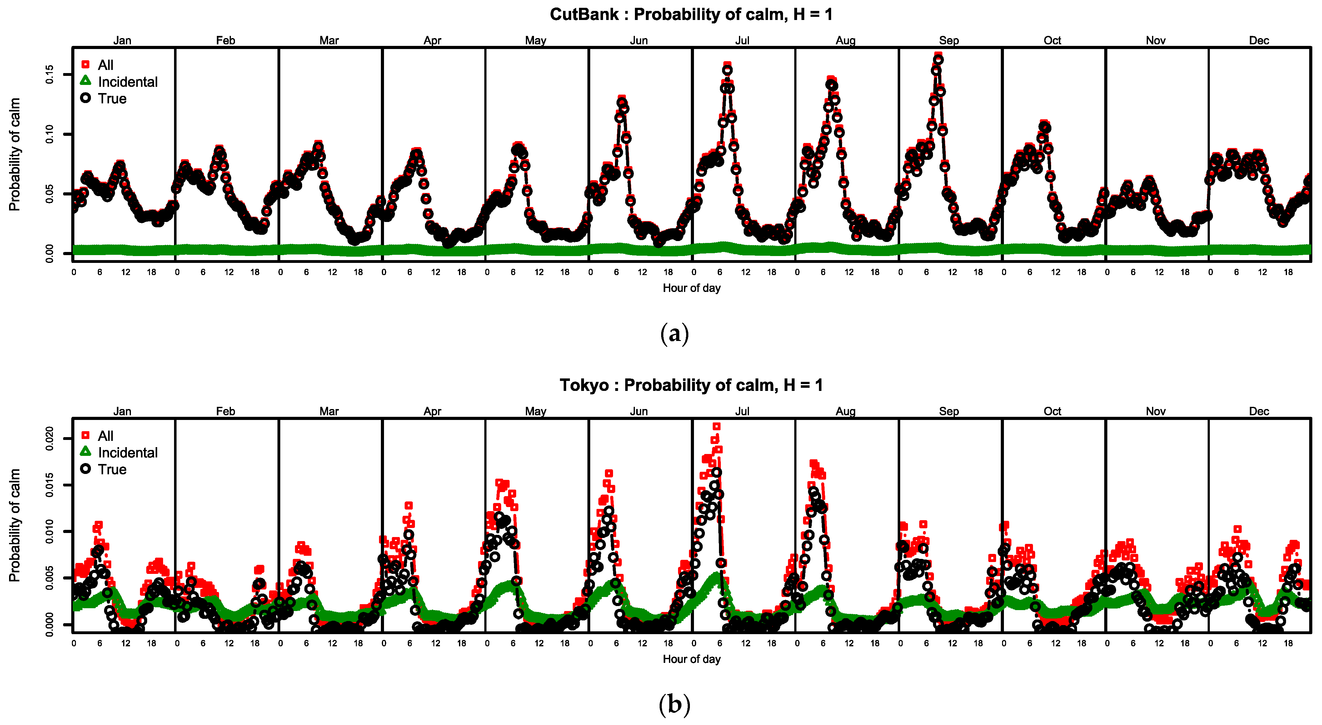
2.2. Calms and Variable Directions

The WMO guide to meteorological observations [15] provides the following definitions:

• Calm: When average wind speed is less than 3 kn.
• Variable direction: When variation from the mean is 60° or more and the current wind speed is less than 3 kn.

Both these states affect the jPDF values near the origin so require resolution, by removing instances of calms and assigning variable directions by interpolation, before the jPDFs can be compiled.

An earlier OEN study [2] proposed that the observed calms consist of

1.

“True calms”: A distinct persistent component of the wind climate, typically comprising over 90% of the observed calms. As these present as a Dirac delta function at the origin of the jPDF, following the Takle and Brown [16] procedure, they were extracted and assessed as a separate component.

2.

“Incidental calms”: A transient occurrence when the vector of a component ellipse happens to pass through the origin. This is the value of $p_{ws}$ at the origin, so it would be counted twice if not removed from the observed calms.

The observed frequency of all calms, f_c, is

$$f_C=f_0+p_{ws}\left(\mathrm{0,0}\right)\times (1-f_0)$$

(3)

from which the frequency of true calms, f₀, is evaluated iteratively.

Typical examples of the seasonal/diurnal variation of calms are shown in Figure 3 for (a) Cut Bank and (b) Tokyo.

2.3. Joint Probability Densities

A compilation of the observed jPDF, $p_{ws}$, at each MH, excluding true calms, was produced by two-dimensional kernel density estimation (2dKDE), replacing the previous binning of speed and direction and polar to Cartesian transformation, which required various intermediate levels of smoothing [4]. The advantages of 2dKDE are that smoothing is uniform across the whole field and controlled by the kernel bandwidth, and that the previous hole at the origin of $p_{ws}$, caused by the exclusion of all calms [4], is automatically filled appropriately. The kernel bandwidth should be large enough to reduce observation variance, but not so large as to over-smooth a significant variation of value. A bandwidth three times the speed increment, i.e., 3 kn, ensures all elements are filled reasonably smoothly in the $p_{ws}$ matrix. A typical observed jPDF is shown in Figure 4a, $p_{ws}$, for MH = 1 at 00:00 in January at Cut Bank. A slight ripple at 10° directional intervals is evident in the outer contours due to light smoothing by the kernel bandwidth.

2.4. Optimizing the OEN Mixture Model

For brevity, the process of optimizing the OEN parameters for the minimum root-mean-square error in $p_{ws}$ (RMSE) is denoted by “fitting,” and the result is found by the “fit”. “Threading” is the process of identifying and indexing each ellipse as it evolves through the MH and was so named because it is equivalent to threading beads of the same color onto the same strand of a multi-stranded necklace. The previous sequential approach [4] of repeatedly adding a new OEN ellipse and refitting until a target quality of fit is achieved, then threading by matching the ellipses to the previous MH, is very slow, because n ellipses require n! fits and threading. It was replaced by a holistic approach that fitted and threaded a fixed number of ellipses without any supervision. This avoided the need in [4] to “remember” ellipses that become insignificant so they could be reintroduced later. Each month was processed independently in parallel under the control of a master script that spawned 12 instances of R and then the results merged upon completion.

2.4.1. Fitting OEN Ellipses to the jPDFs

In the previous implementation [4], the jPDFs were pre-smoothed by a Gaussian kernel filter applied to preceding and succeeding hours and months to make the supervised fitting less onerous. In this study, the observed jPDFs were fitted in three stages, by month in parallel, with threading of the whole year between each stage. In the first stage, fuzzy clustering was applied to each jPDF to estimate the membership probability of each ellipse. The initial parameters evaluated from the probability-weighted moments, i.e., from the “fuzzy OEN” of the original method [4], were approximated in one step. In the second stage, initial parameters were reset to the frequency-weighted mean parameters for each month, and in the third stage, initial parameters were reset to the best-fitting neighbor MH to eliminate the occasional outlier. After each fitting stage, any out-of-bound ellipses were culled, and the remaining ellipses were refitted. No additional smoothing was used through this process to avoid masking sudden changes, e.g., the onset of monsoon.

Figure 5 shows how the fit for Delhi improves through the fitting stages in terms of $R^2$. In (a), the black circles are the first-stage values, and the red squares are the improved second-stage values. In (b), the black circles are the second-stage values, and the red squares are the improved third-stage values. The improvement in $R^2$ is modest overall but is largely by improving the poorest fits. The incidence of out-of-bound values decreases through each stage. The fits for this location are poorest at the start of the summer monsoon, May–June, and indicate variability in the date of onset.

Figure 4b shows a typical optimized fit of eight ellipses for MH = 1 (00:00 in January) at Cut Bank. As the ellipses were sorted by overall frequency in decreasing order, their indices rank the relative importance of each ellipse. This station has the highest incidence of winter “interior Chinook” foehn winds within the contiguous USA, which appear in the WSW components represented by the line of ellipses: 5, 6 and 7. The OEN model reproduces the observed tri-modal pattern in Figure 4a, smoothing the ripples in the outer contours, achieving a Pearson correlation of $R^2=0.995$ and $\mathrm{R}\mathrm{M}\mathrm{S}\mathrm{E} = 2.71\times {10}^{-5}$, indicating an excellent fit.

Figure 6a shows the corresponding QQ plot of the observed and OEN model jPDFs, $p_{WS}$, for all MH. The (black) circles show the fitted values, where the error scatter is least in the high-valued body and greatest in the low-valued tails, as might be expected, with an overall fit accuracy of $R^2=0.995$ and $\mathrm{R}\mathrm{M}\mathrm{S}\mathrm{E} = 2.76\times {10}^{-5}$. Figure 6b shows the corresponding QQ plot for the OSN model, introduced later.

The expectation from earlier studies [1,2,3,4] is that the OEN model accuracy should improve with an increasing number of ellipses. Considering physical meteorology, the number of ellipses should ideally match the number of unconstrained wind components. With more ellipses, some components will be represented by more than one ellipse if this improves the overall fit; otherwise, the redundant ellipses will tend towards insignificance [4]. Figure 7 presents the overall goodness-of-fit (GOF) metrics, $R^2$ and RMSE, over the range from 4 to 14 ellipses, for five stations. The trends take a similar shape for all stations, although the values vary with the differing quality of the observations. There appears to be little advantage to be gained by fitting more than eight ellipses, which is why eight are used here as the datum for reporting, while there are indications that fit accuracy diminishes with more than 12 ellipses. Figure 8, for Tokyo, shows the variation of $R^2$ and RMSE with MH using eight ellipses, indicating more diurnal variation of GOF in the winter monsoon than in the summer. The solid curve represents a 3 h running mean cycling over each month. The values of the GOF metrics reflect the balance between the observational variance remaining in $p_{ws}$ and model error in fitting OEN. Increasing kernel bandwidth in evaluating the observed $p_{ws}$ by KDE improves GOF at the risk of over-smoothing.

2.4.2. Unsupervised Threading of the Ellipses

In the original sequential method [4], any error made in threading persisted and propagated forward to later MH, requiring tedious manual inspection and correction. Instead, the new method operates holistically on the parameters for all MH, again in three stages. In the first stage, fuzzy k-means clustering is applied to the ellipse centers, W and S, to obtain the center of each ellipse cluster, which are normalized by their mean and standard deviation to give a datum pattern. The pattern of ellipse centers for each MH, similarly normalized, is sorted by the closeness of each ellipse to the datum pattern in increasing order of separation distance. This provides an initial threading that takes no account of seasonal variation. In the second stage, this process is repeated using the datum pattern formed from the frequency-weighted mean W and S for each month, which allows for seasonal variation. Where ellipses overlap, these two stages ensure that the ellipses are correctly threaded when they separate. The final stage takes account of the scale and orientation of each ellipse in addition to the location by matching the intersection areas of each ellipse, ensuring the best match while ellipses overlap. By eliminating manual inspection and correction, this represents the most significant advance over the original method [4], reducing threading time from many hours to a few seconds.

Figure 9 demonstrates the effectiveness of the unsupervised threading process in resolving the mean zonal–meridional components, $W$ and $S$. Tokyo was chosen as the example for the strong sea/land breeze diurnal oscillations and the seasonal changes between the summer and winter monsoon, which are gradual at the winter–summer change but abrupt at the summer–winter change (October–November). The color key indexing individual ellipses is used consistently in reporting this study.

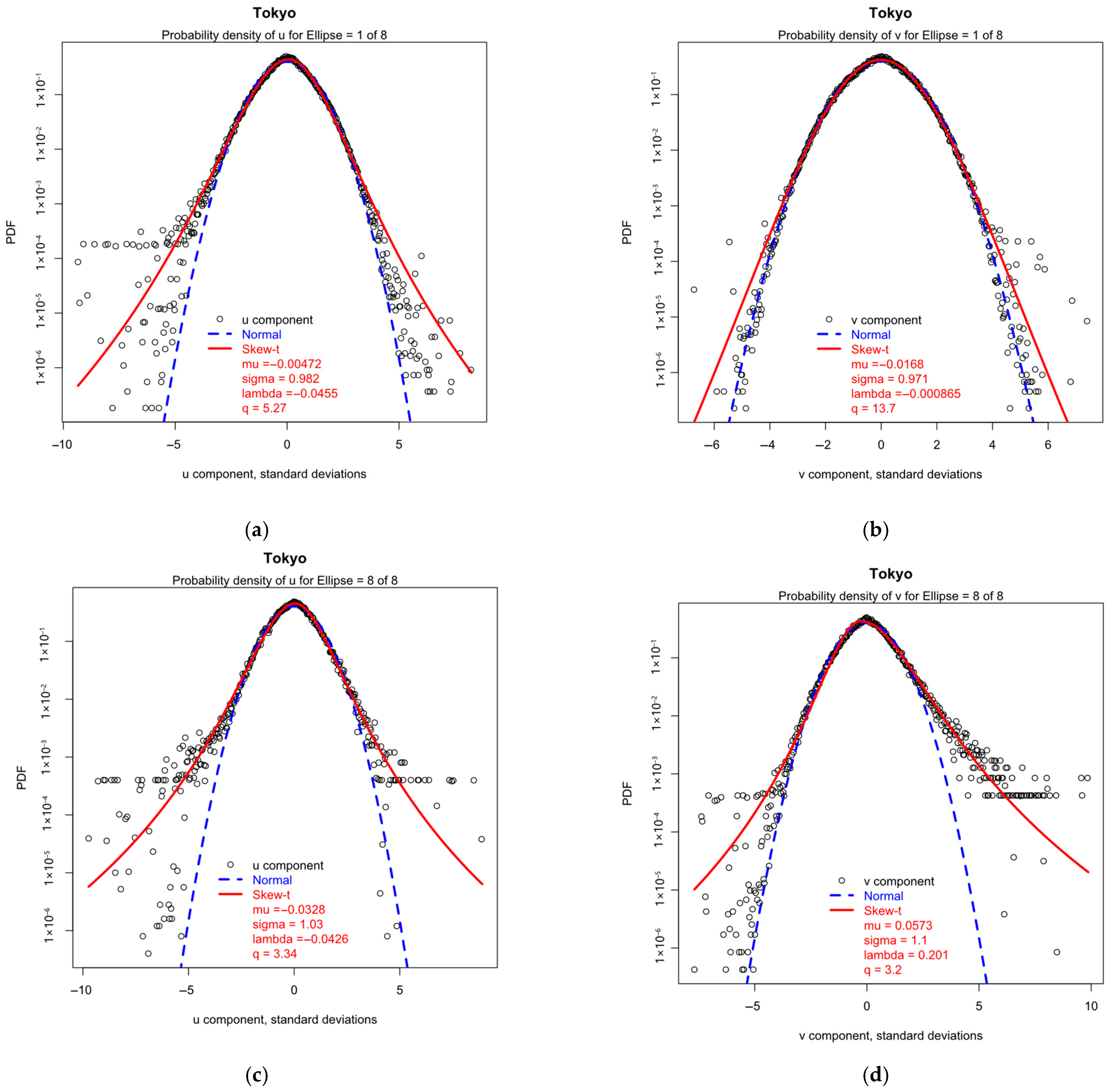
2.5. Assessing Deviations from Normal

The previous study [4] introduced a method to demodulate the seasonal–diurnal variation of the orthogonal vectors, normalized as $u/{\sigma }_u$ and $v/{\sigma }_v$, and then evaluate their PDFs from the fuzzy probability (membership ratio) of each ellipse. By the theory underpinning the OEN model [6,7,8,9], all should collapse onto the standard normal distribution.

Figure 10 presents the PDFs of the demodulated $u/{\sigma }_u$ and $v/{\sigma }_v$ for all MH from the eight-ellipse OEN model for Tokyo: (a, b) of the most dominant ellipse 1; and (c, d) of the least dominant ellipse 8. Observations are reasonably normal over 3 orders of magnitude (OM) for ellipse 1, but only 2 OM for ellipse 8. Further into the tails the observations deviate above normal. As all the other stations show the same trends, the question arises as to whether this indicates deficiencies in the OEN model or in the demodulation process.

A possible reason for a deviation from normal is insufficient degrees-of-freedom, $n$, for convergence by the Central Limit theorem. The Student t-distribution generalizes the normal distribution for finite degrees of freedom, $n$. It is asymptotic to normal as $n\to \infty$and to the Cauchy distribution as $n\to 2$, remaining symmetrical throughout this range [10]. Further generalization into the Skew-t distribution is obtained by admitting skew [17], which is implemented in R (Version 4.4.1) by several packages. The “sgt” package (Version 2.0) was adopted here because this conveniently retains the mean and standard deviation as parameters, with the other relevant parameters being as follows: $-1\le \lambda \le 1$ expressing skew, and $2\le q\le \infty$ expressing $n$. The optimal Skew-t parameters in Figure 10 provide very low values of $q$, suggesting only a few degrees of freedom, which is physically unrealistic.

A close inspection of Figure 10 shows that the observations in the tails tend to split into two sets: one set following the normal tail and the other diverging above, with the balance favoring normal for ellipse 1 and divergent for ellipse 8. This strongly suggests that the normal set belongs to the target ellipse and the divergent set belongs to fuzzy contributions from the other ellipses, i.e., the expected “leakage” [4] in the demodulation process. Ellipse 1 performs better than ellipse 8 due to its higher dominance through its greater relative frequency.

Confirmation of this suggestion required fitting the bivariate Skew-t mixture model (SGT) directly to the jPDFs to assess the effect of skew and kurtosis completely independently of the demodulation process. Two issues arise:

1.

It is impractical to use the Crutcher model with SGT because admitting skew and kurtosis requires expanding the single correlation parameter ${\rho }_{ws}$ into a 3 × 3 correlation matrix to account for the additional central cross-moments. It is simpler and more convenient to use the Harris model and add the $\lambda$ and $q$ Skew-t parameters.

2.

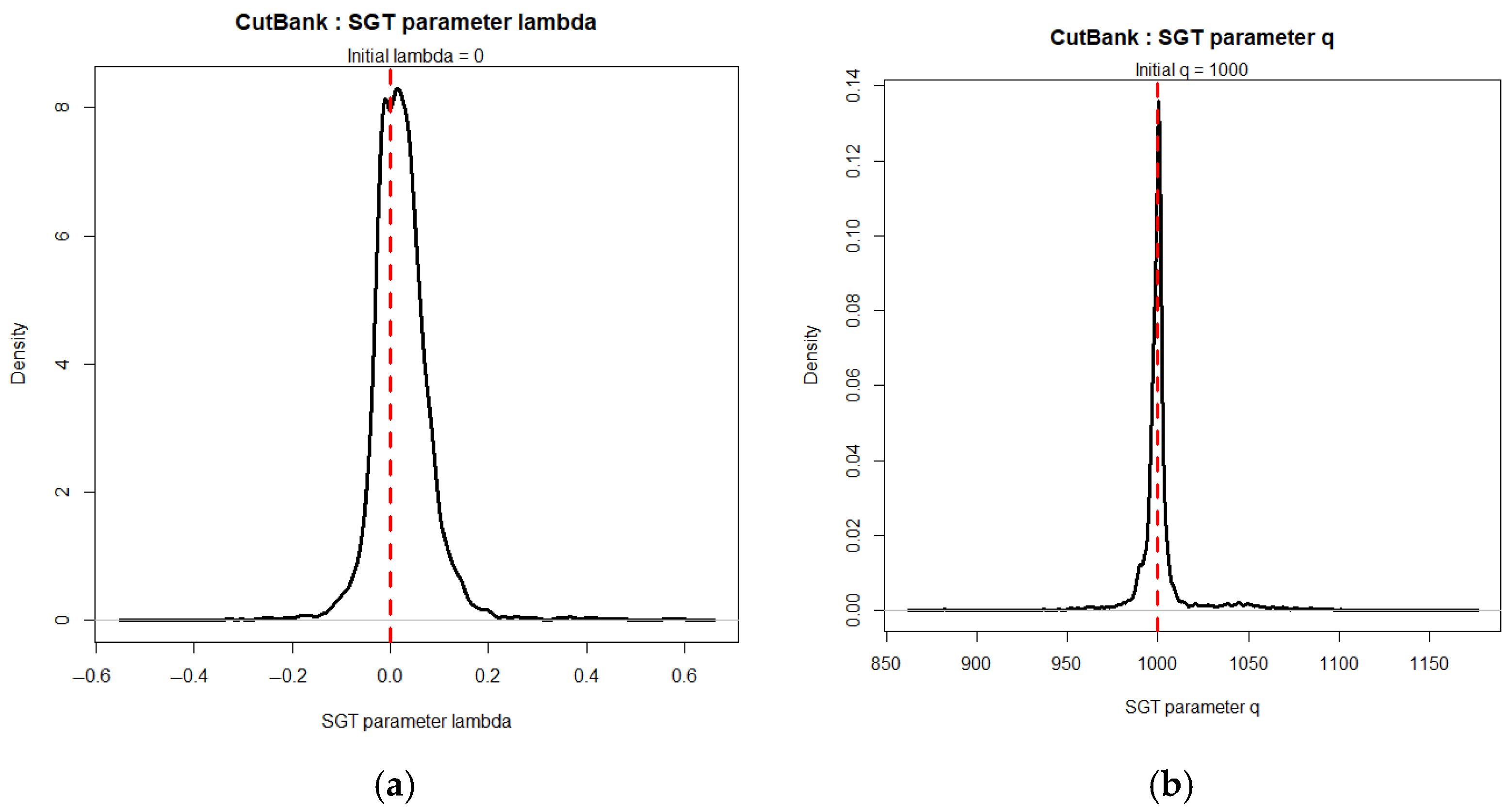
In initializing the SGT fits with parameters transformed from the previously fitted OEN, the normal values $q_u=q_v=\infty$ must be substituted by finite values, large enough to be effectively normal, for the optimization to work. Here, $q_u=q_v=1000$ was used, giving an initial standard error of $\epsilon =5.38\times {10}^{-5}$.

Figure 11 presents the distributions of $\lambda$ and $q$ for all ellipses and MH at Cut Bank. In (a), $\lambda$ moves from zero to small positive or negative values, resulting in a bimodal distribution with a sufficient spread of values to indicate skew has some small influence. On the other hand, in (b), $q$ remains centered on the initial value, with minimal spread, indicating no significant excess kurtosis. This also applies to the other locations, confirming that the deviations in the tails of Figure 10 are indeed artefacts of the demodulation process, but that the body of distributions can exhibit mild skew. Normality through the Central Limit theorem predicts a zero skew asymptote and unlimited tails to the jPDF. Some of the meteorological wind-producing mechanisms are physically limited in the lower tail to zero, e.g., sea breezes are always onshore and katabatic winds always downslope, while their upper tails remain unlimited. In these cases, some degree of skew is inevitable and does not violate the physical justification for the OEN model.

2.6. OSN: The Offset Skew Normal Mixture Model

A consequence of admitting four additional parameters, ${\lambda }_u$, ${\lambda }_v$, $q_u$and $q_v$, into the SGT fit is that it takes 16 times longer than the OEN model to optimize the same number of iterations. As excess kurtosis is seen to be insignificant, it makes sense to exclude this from optimization. This leads directly to the Offset Skew Normal (OSN) mixture model by setting $q_u=q_v=\infty$ as constants. With just two additional free parameters, ${\lambda }_u$, ${\lambda }_v$, the fitting time of OSN is four times that of OEN for the same number of iterations. It is convenient to initialize the OSN fit with the threaded OEN parameters transformed from Crutcher to Harris and with ${\lambda }_u={\lambda }_v=0$, then to refit and re-thread, omitting the first fuzzy-clustering stage.

3. Results

3.1. Principal Aims

As the principal aims of this study are to report improvements to the accuracy and applicability of the OEN mixture model while maintaining the links to physical foundations, the reporting of results is confined to demonstrating whether these aims were achieved. Fuller results are provided as Supplementary Figures S1–S112. The extension of OEN into OSN by admitting skew, supported by upgrading the R scripts to accept both Crutcher and Harris parameters, collectively forms an extended OEN model. This is now denoted by XOEN when applicable generally to both models but as OEN or OSN when applicable exclusively to the respective model.

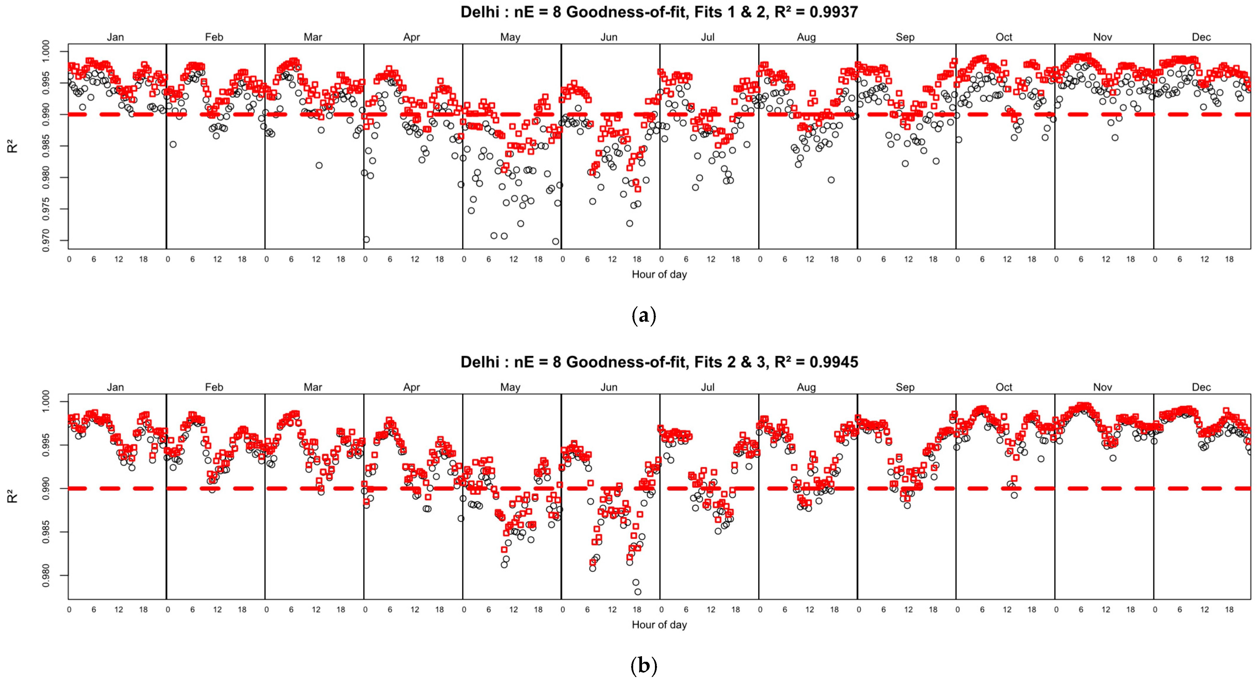
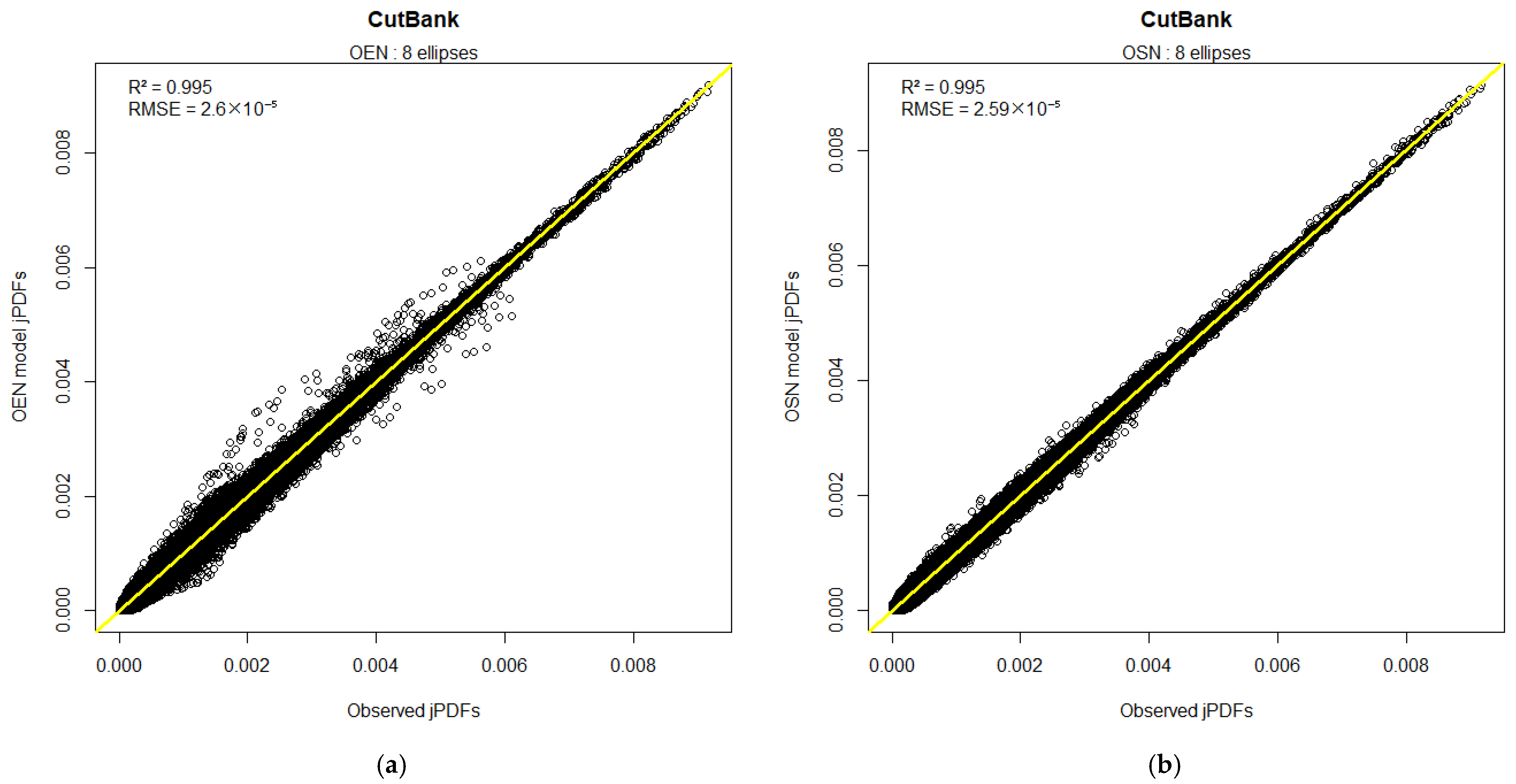
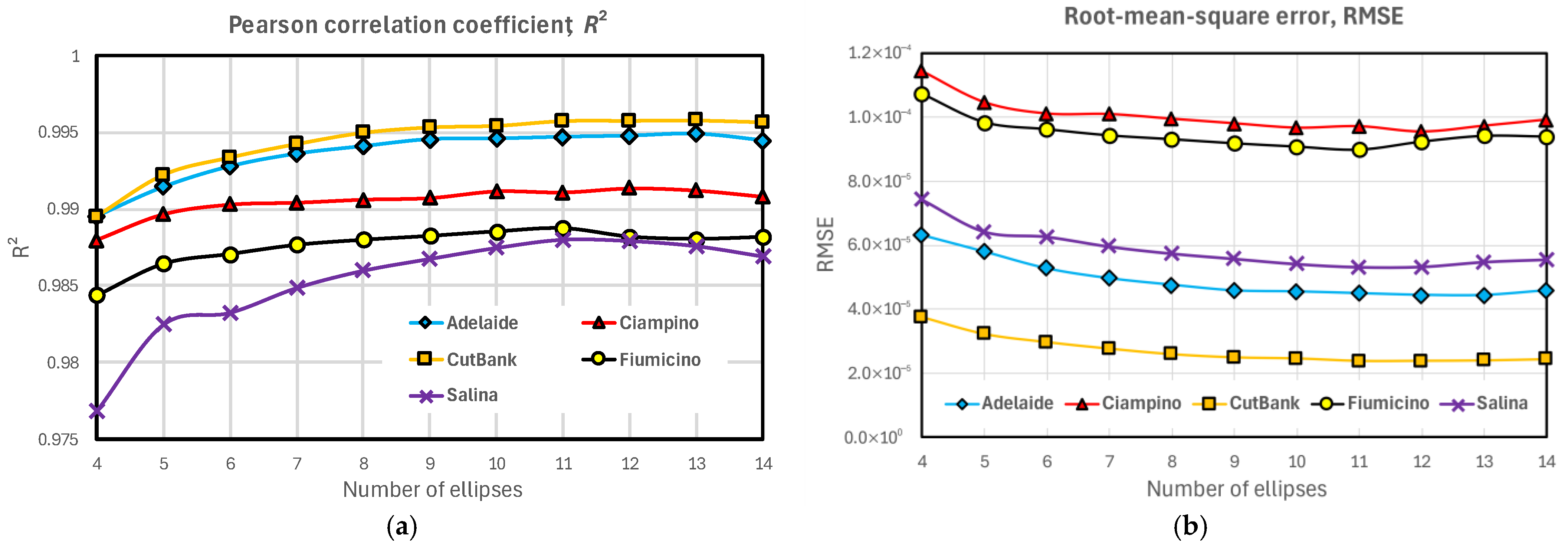
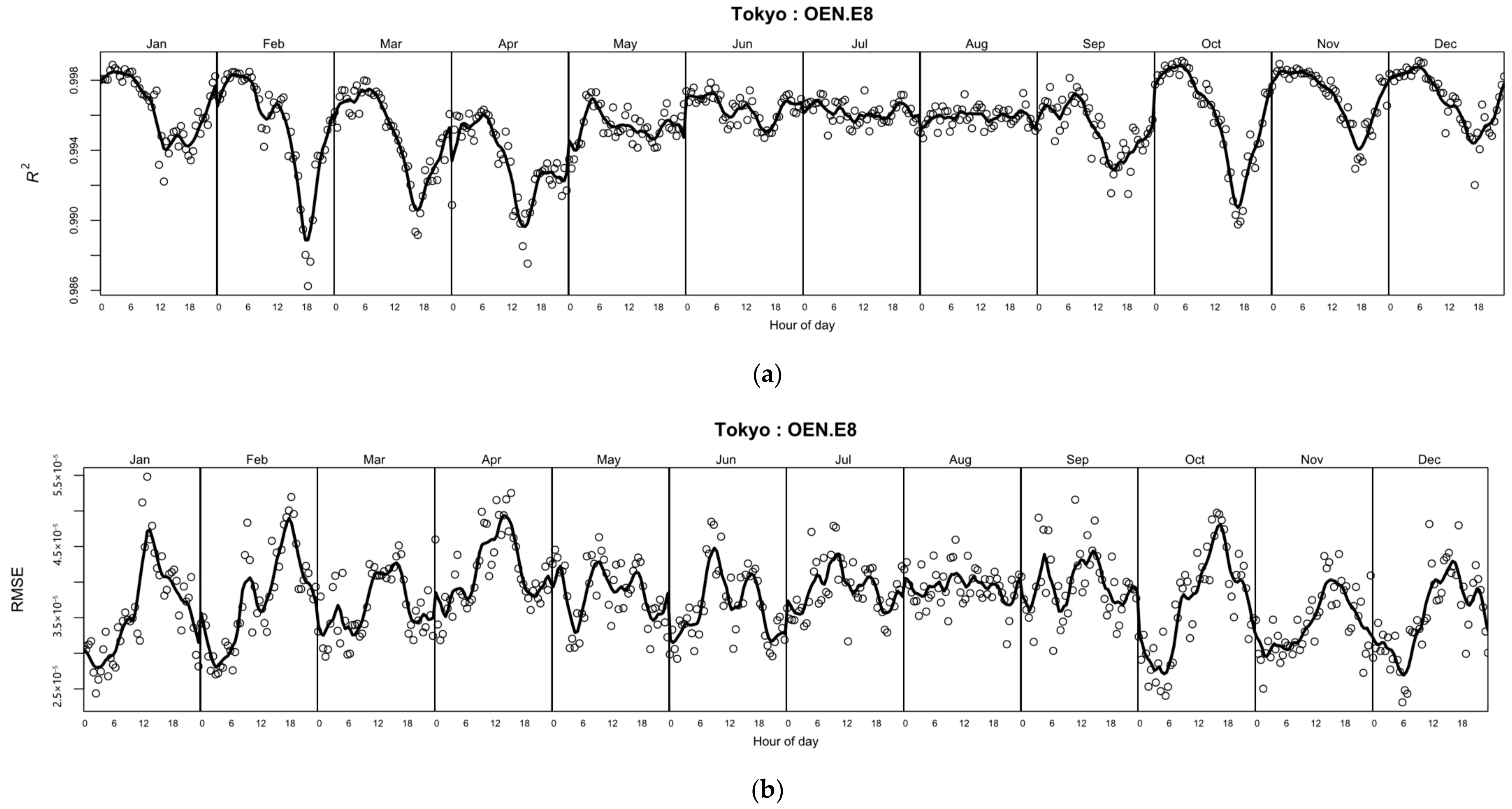
3.2. Goodness of Fit Metrics: R² and RMSE

Figure 12 compares the goodness of fit (GOF) metrics, $R^2$ and RMSE, of the XOEN mixture models for the eight-ellipse fits at all stations in this study, ranked by increasing GOF. This shows improvements for OSN over OEN at all stations, larger in $R^2$ for the poorer-fit stations but aways marginal in RMSE. The reduced scatter in Figure 6b shows most of this improvement is in the low values of the jPDF. Note that the stations rank in a different order for $R^2$ than for RMSE: $R^2$ expresses the consistency of the fit while RMSE expresses the residual error, which conflates model error with the observational variance.

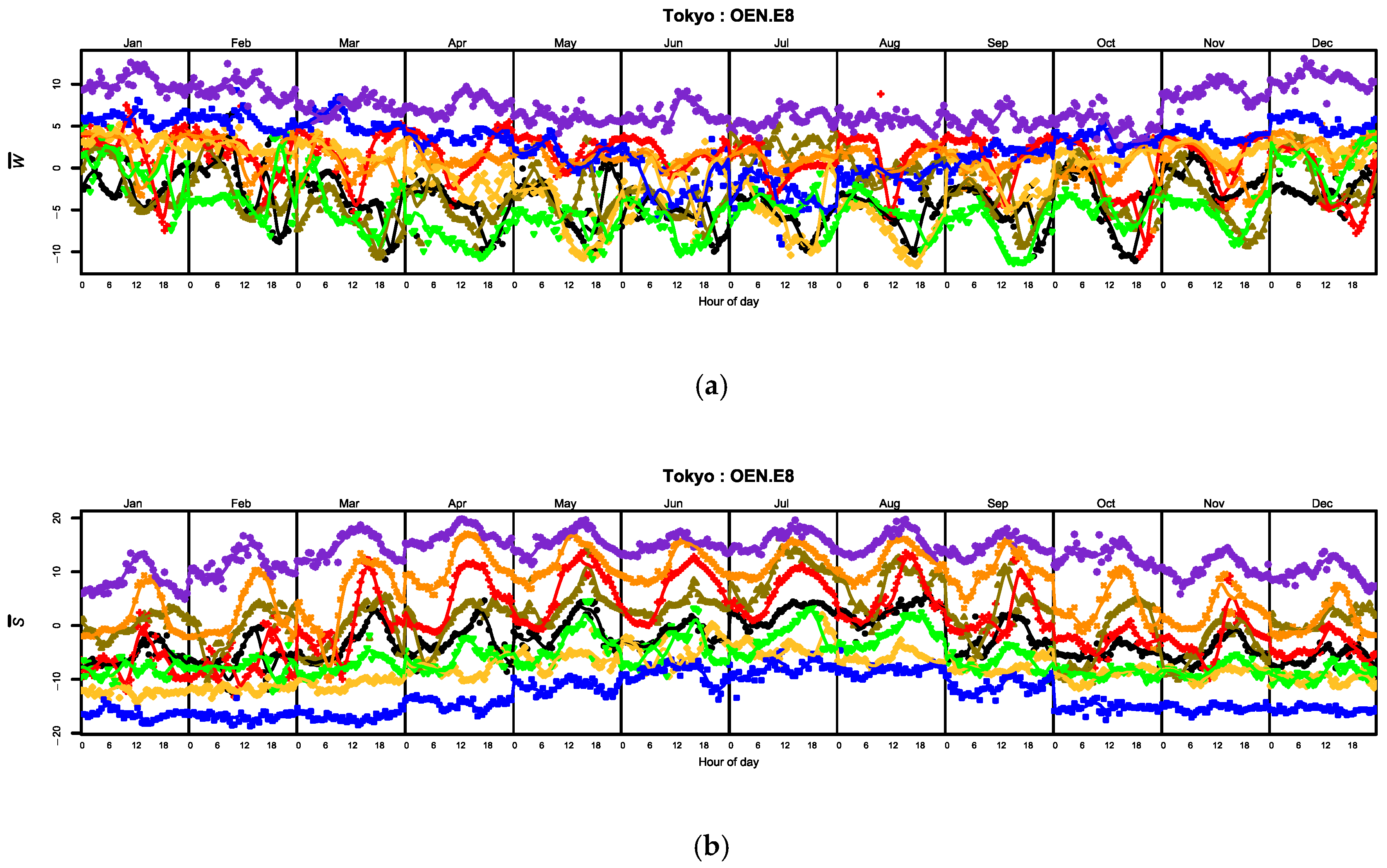
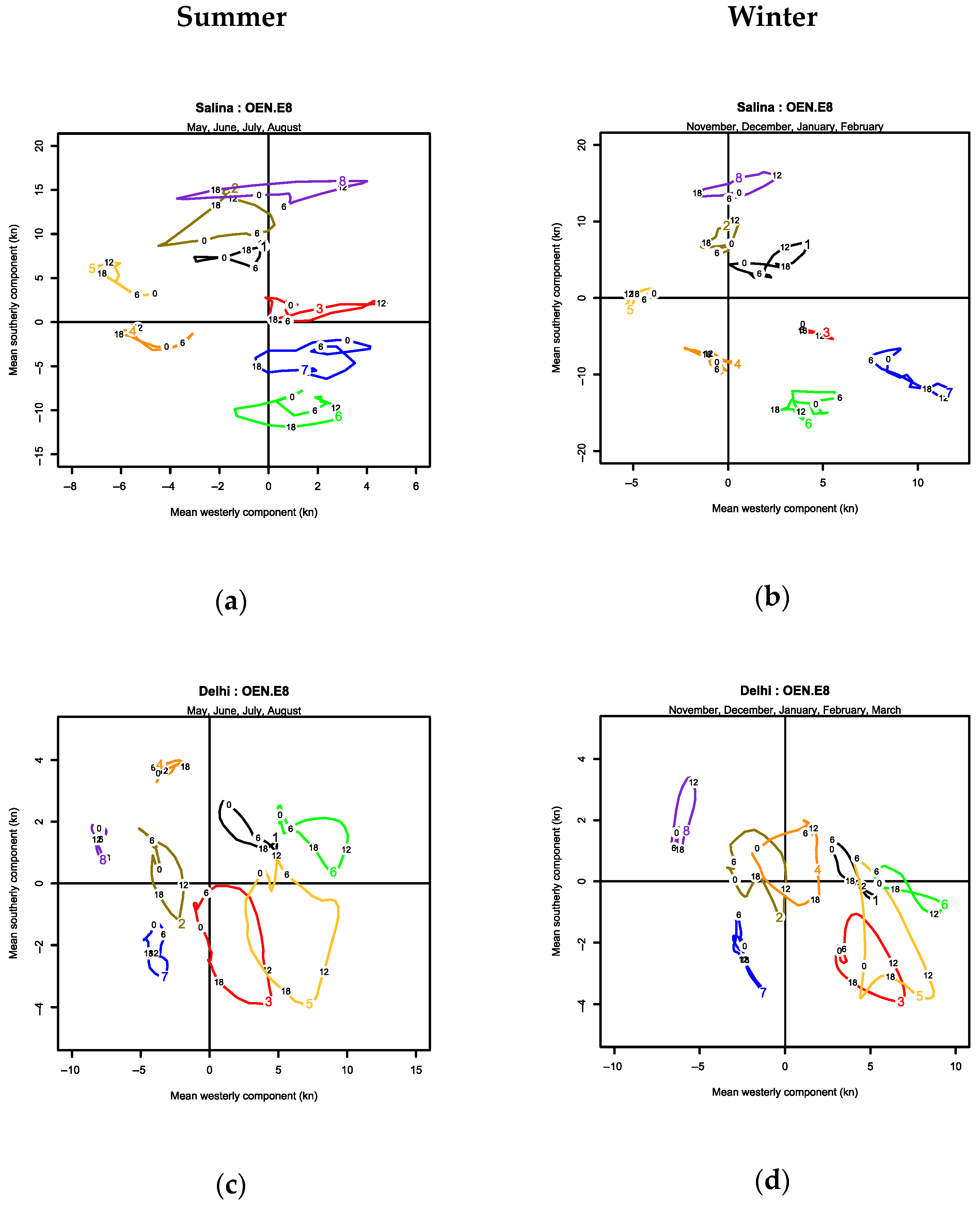
3.3. Diurnal Hodographs of the Mean Vectors

Diurnal hodographs of the mean vectors are useful in deducing the physical meteorology driving each XOEN ellipse, indicating consistency for a given ellipse and whether two or more ellipses share a single mechanism. These hodographs have proved useful in the study of the sea/land breeze cycle—from the theory proposed by Haurwitz [18], which predicts that they form open loops that progress clockwise in time in the northern hemisphere and anticlockwise in the southern, to its application at various locations [19,20,21,22,23,24]. This confirms Haurwitz theory at coastal locations where the weak Coriolis effects are not overwhelmed by other factors, such as coastal orography that can reverse the direction [25] or present as a figure-of-eight loop. On the other hand, directionally constrained mechanisms such as katabatic winds present as closed linear loops.

Figure 13 shows the diurnal OEN hodographs for the metastable summer (left) and winter (right) periods at locations selected to illustrate specific aspects of physical meteorology.

3.3.1. Salina

Salina represents a location free of any topographic constraints since it lies in the Great Plains at the geographical center of the contiguous USA and is far from any mountain range or coastline. It also lies on the boundary of the Koeppen–Geiger major climate classes: “Cold” to the north and “Temperate” to the south ([26] Figure 8b). As seen in Figure S15, the principal synoptic-scale winds are from the NNW and the south, with NNW dominating in winter and south in summer, which is reflected in the difference between Figure 13a,b. Diurnal wind speeds occur throughout the year, showing a consistent trend in most ellipses of a small westerly deviation, building to a maximum at noon, consistent with the insolation cycle. The loops are generally closed but, where they are open (e.g., ellipse 2 in summer), the direction is the opposite to the Haurwitz [18] theory. The closed loops are not aligned in the same direction, indicating freedom from directional constraints.

3.3.2. Delhi

Delhi represents a weak monsoon location, where the wind climate switches between two distinct states, as seen in Figure S29. Delhi is too far inland for any sea/land breeze component and, at about 200 km SW of the Himalayan range, is not subject to katabatic winds. The loops of most ellipses in Figure 13c,d are open and progress clockwise, as expected [25] for the location at 28.7° N, but with major axes generally aligned with the Himalayan range, indicating significant orographic steering of the synoptic-scale weather systems.

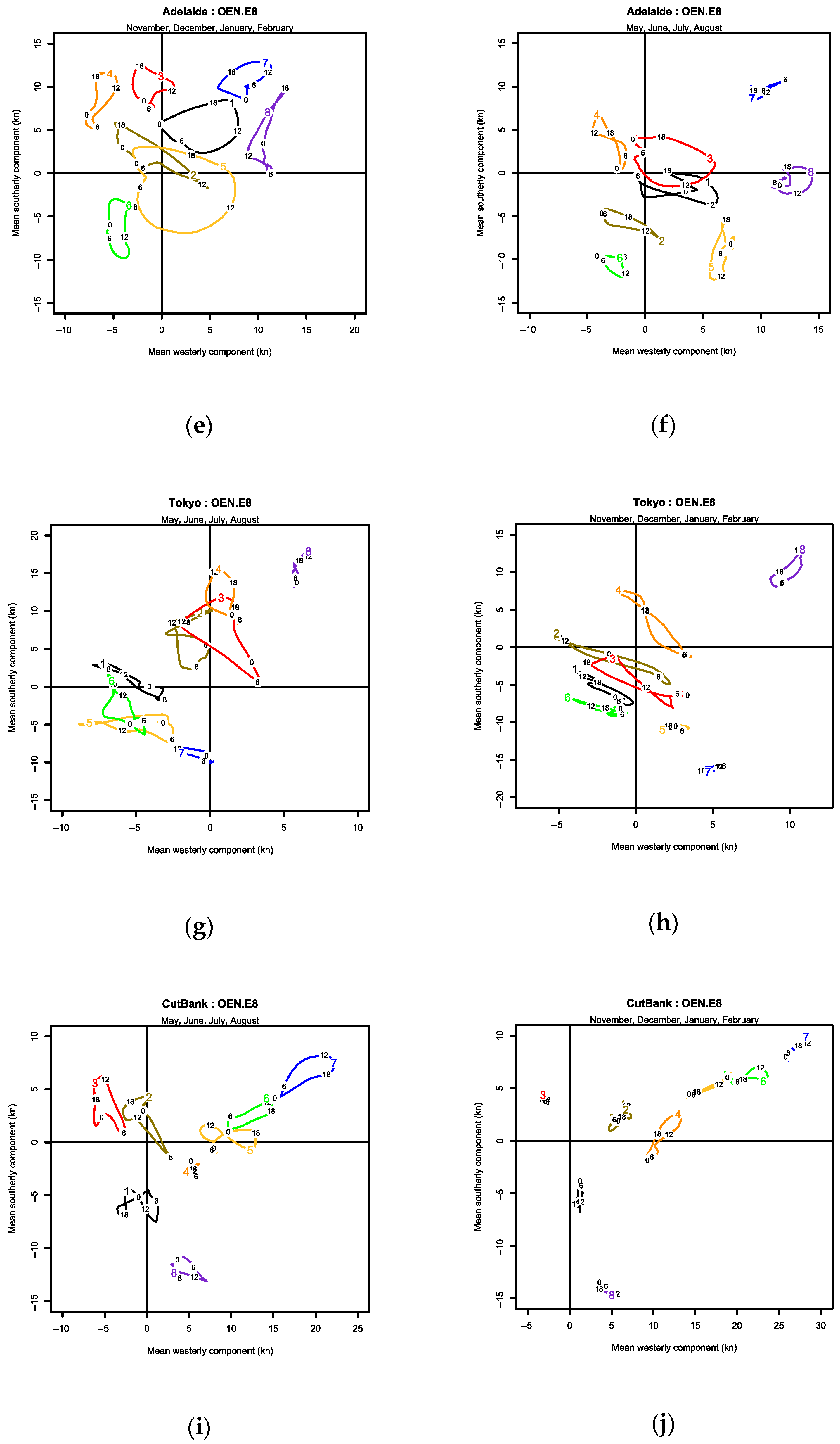
3.3.3. Adelaide

Adelaide lies between the western shore of the Gulf of St Vincent and the Mount Lofty ranges to the east, along the SW-facing continental coast of South Australia, and represents a location with strong sea/land breeze components. As seen in Figure S1, distinctly different summer and winter characteristics, driven by the seasonal migration of the sub-tropical ridge [2], are similar to a monsoon climate. This well-studied wind climate [27,28,29,30] is a complex mixture of synoptic-scale weather systems, local- and continental-scale sea/land breeze components and orographic winds. The diurnal transition from local to continental see breezes presents as two peaks, at 230° and 160°, in summer. This was parameterized by the original OEN methodology [2] using five ellipses representing non-diurnal summer and winter synoptic-scale components, diurnal sea and land breeze components and a diurnal downslope “gully wind” [30] component. The ellipses in Figure 13e,f are generally open and all progress anticlockwise, as expected for the southern hemisphere [25], maximizing a westerly component shortly after local noon. Any suggestion that ellipses 2 and 4, which overlap in summer, could represent a single mechanism is contradicted by their separation in winter. The sea breeze component in the previous OEN model [2] turns from westerly, normal to the local coastline, to southerly, normal to the continental coastline as each day progresses. Here, in the summer, the sea breeze appears to separate into ellipse 1, as the dominant continental component, and ellipse 4 as the local component; in the winter, ellipse 1 is the dominant local component and ellipse 3 is the continental component.

3.3.4. Tokyo

Tokyo represents a location with strong sea/land breeze components within a monsoon-dominated climate. The change between winter and summer monsoon is sudden, and the respective characteristics are almost exclusive, as seen in Figure S43. Lying on a west-facing coast, the sea breeze builds to a maximum easterly just after noon. These sea breeze components are strong in summer, seen in the open anticlockwise loops in Figure 13g, against the expectation of [25], and weaker in (h) in winter. The superposition of two pairs of ellipses, 1–6 and 2–3, suggests each pair may be a single mechanism.

3.3.5. Cut Bank

Cut Bank in Montana, USA, represents a location dominated by orography, as it lies close to the foot of the Rocky Mountain chain, which steers the synoptic-scale weather systems along an NNW-SSE axis and generates katabatic winds normal to this axis. While classical cold katabatic winds occur throughout the year, the location is notable as it has the highest incidence within the contiguous USA of foehn, or “interior Chinook”, warm dry winds (the highest incidence being at Lethbridge, Alberta, Canada, 125 km to the north), which is a winter phenomenon. Except for ellipse 3, which forms an open anticlockwise loop in summer, the other loops are generally small or linear and closed. Their centers in Figure 13i,j form a rotated “T” pattern, with the steered NNW-SSE components as the top bar of the “T” and the tail pointing ENE representing the katabatic components (ellipses 5–7). The katabatic components present in Figure S57 as a narrow band of wind direction around 250°, while a weaker diurnal increase in wind speed in summer after noon presents as a diffuse band around 140°.

3.3.6. Halley Station

Halley, lying on the Brunt Ice Shelf of Antarctica, represents a coastal location dominated by orography that is virtually devoid of diurnal variation since it alternates between six months of continuous day and six months of continuous night. This greatly simplifies how component ellipses present on the hodographs as patterns in Figure 13, which remain consistent between summer, (k) and winter (l) seasons, albeit at different relative strengths. Weak onshore components (ellipses 4 and 7) and strong katabatic offshore components (ellipses 3, 5, 6 and 8) lie along the same axis, normal to the coastline and orography. The katabatic components present in Figure S71 as a narrow band of wind direction around 70°, and the on-shore components present as a complementary diffuse band around 250°. The most frequent ellipse 1, which lies off this axis, is assumed to be driven by the circumpolar vortex, and the second most frequent ellipse 2, is assumed to represent a weak land breeze or drainage flow.

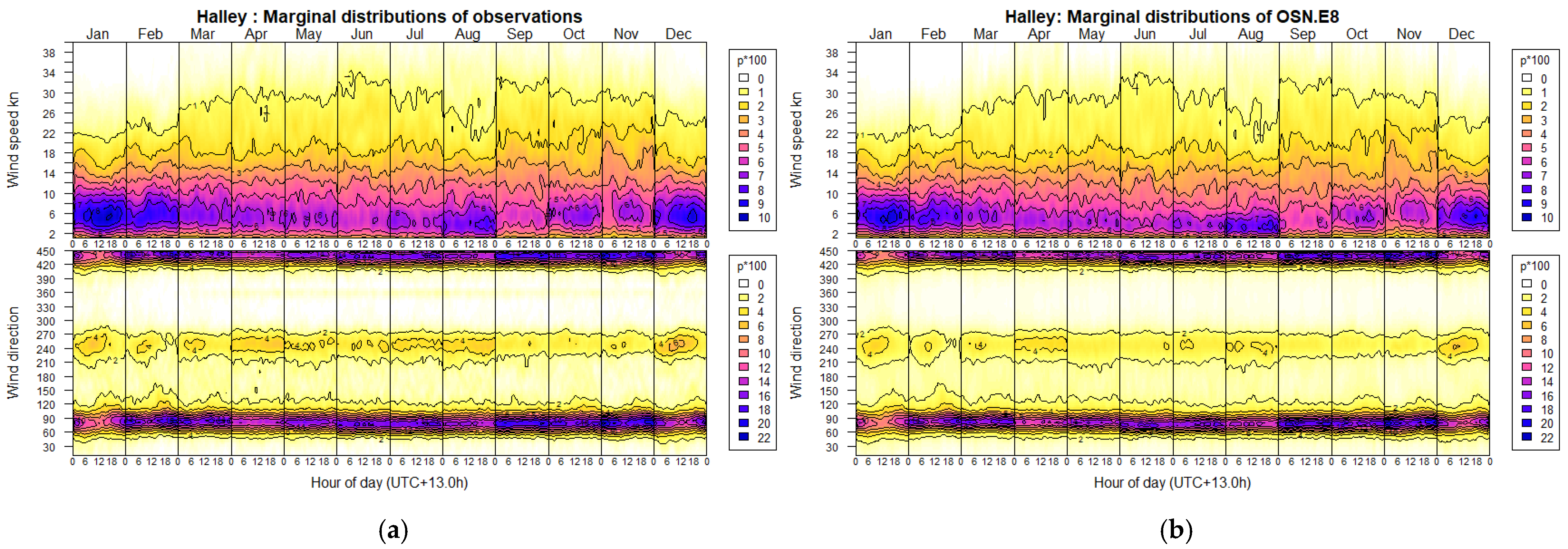
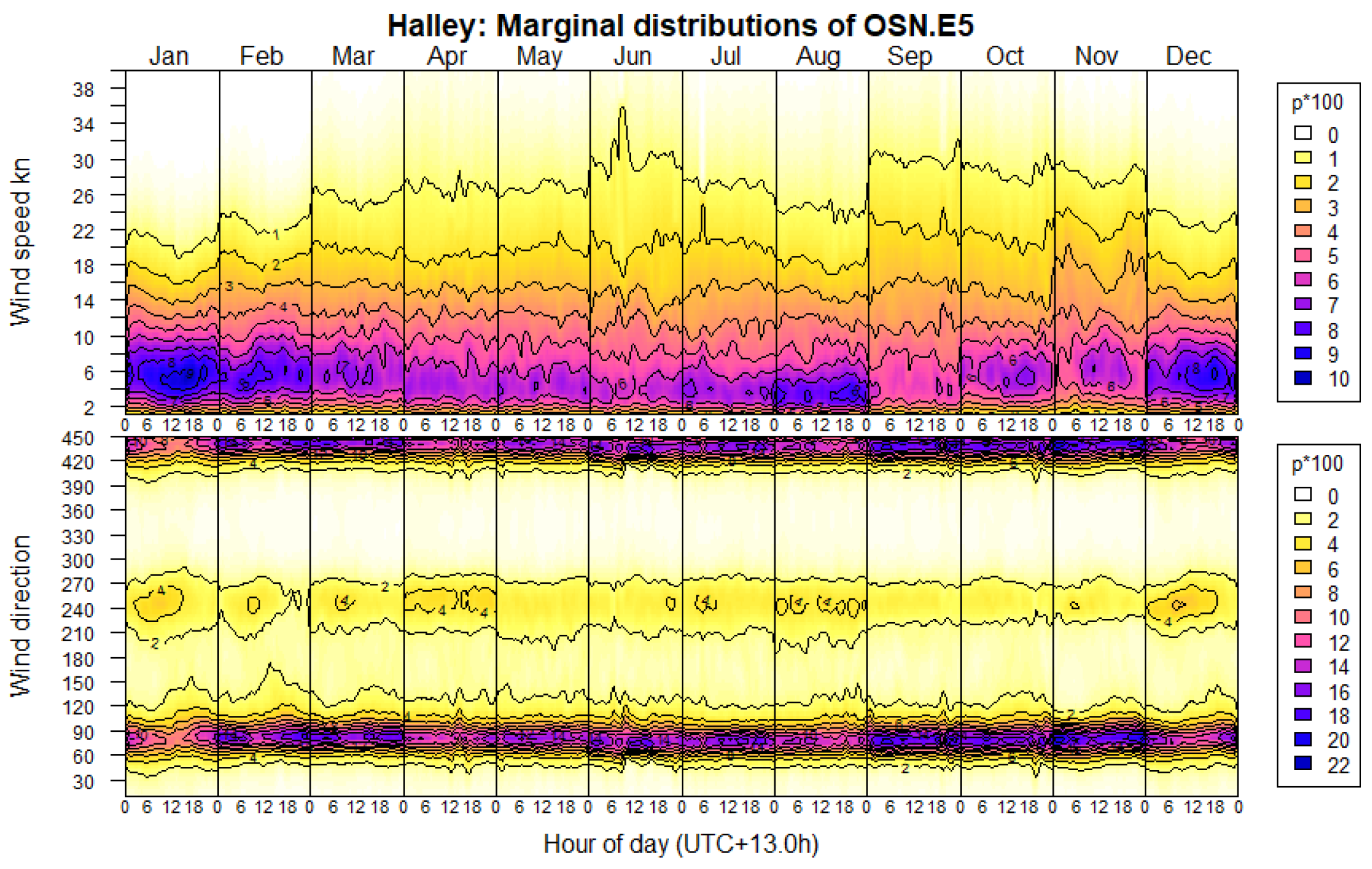
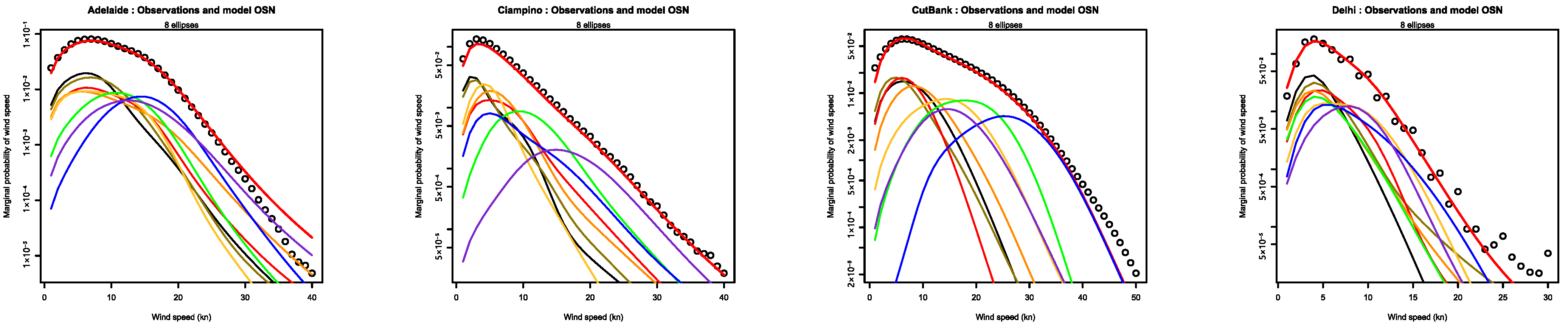
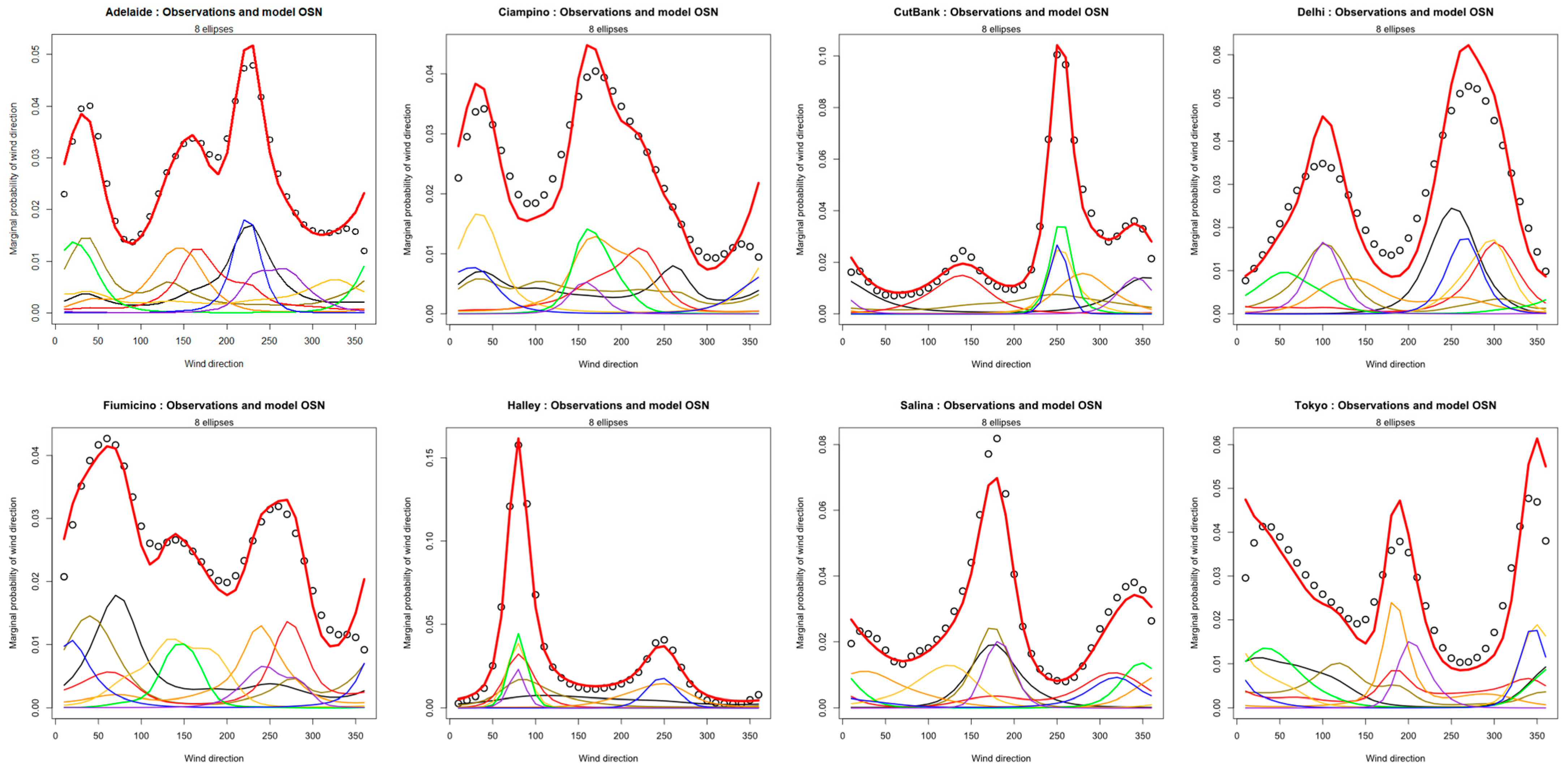
3.4. Marginal Wind Speed and Direction Distribution Charts

Charts of the marginal pdfs, $p\left(V\right)$ and $p\left(\theta \right)$, of wind speed and direction at each location are included in the Supplementary Figures for the following: observations, eight-ellipse OEN model and eight-ellipse OSN model. These are in the format introduced in [31] to visualize the seasonal–diurnal trends in a single chart. The charts for Halley Station in Figure 14 show that the marginal distributions in (b), evaluated from the OSN model, are a faithful, smoother representation of the observed distributions in (a).

3.5. Postscript

Collating these results with the fuller set in Supplementary Materials revealed that, as the goal of the revised OEN/OSN methodology is to minimize RMSE using a predetermined number of ellipses, when splitting is more advantageous to this goal, a dominant ellipse will split in two in preference to defining a new minor ellipse. Nevertheless, elements of physical meteorology remain recognizable in the resulting shared ellipses. Diurnal sea/land breeze and seasonal monsoon cycles do not appear to constrain wind direction enough to affect the justification for the OEN/OSN model. However, the tight directional constraints of the katabatic components resolve as multiple ellipses centered along a common axis to form an empirical Gaussian mixture. Initializing the OSN fit by the OEN ellipses limits the degree of skew introduced into each ellipse because the fit follows the error gradient to the nearest local minimum, whereas merging the katabatic ellipses into a single highly skewed ellipse might provide a better solution. This proposition is tested in the following section.

4. Rationalizing the XOEN Ellipses

4.1. Reason for Rationalization

As noted above, when fitting a fixed number of ellipses, sufficient for all significant ellipses to be detected, the optimization process may split a dominant ellipse into two ellipses in preference to resolving a minor ellipse and will resolve katabatic components as a set of directionally aligned ellipses. In addition, ellipses of mechanisms that become rare produce outlier parameters or are substituted by the next-best ellipse, which is typically quite different. This was prevented by supervision in the original method [4] and represents the price paid for the large reduction in analysis time and for eliminating the possibility of observer bias. This leaves the issue of identifying ellipses for rationalization by merging splits or removing redundancies.

4.2. Katabatic Components

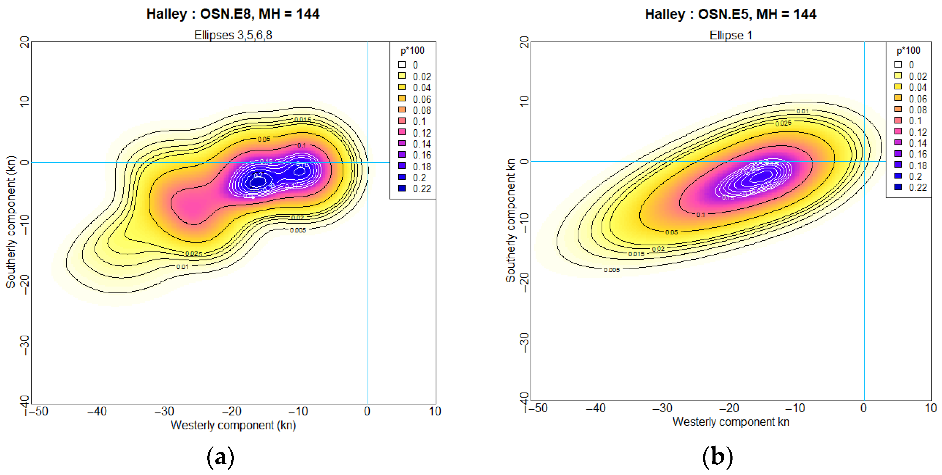
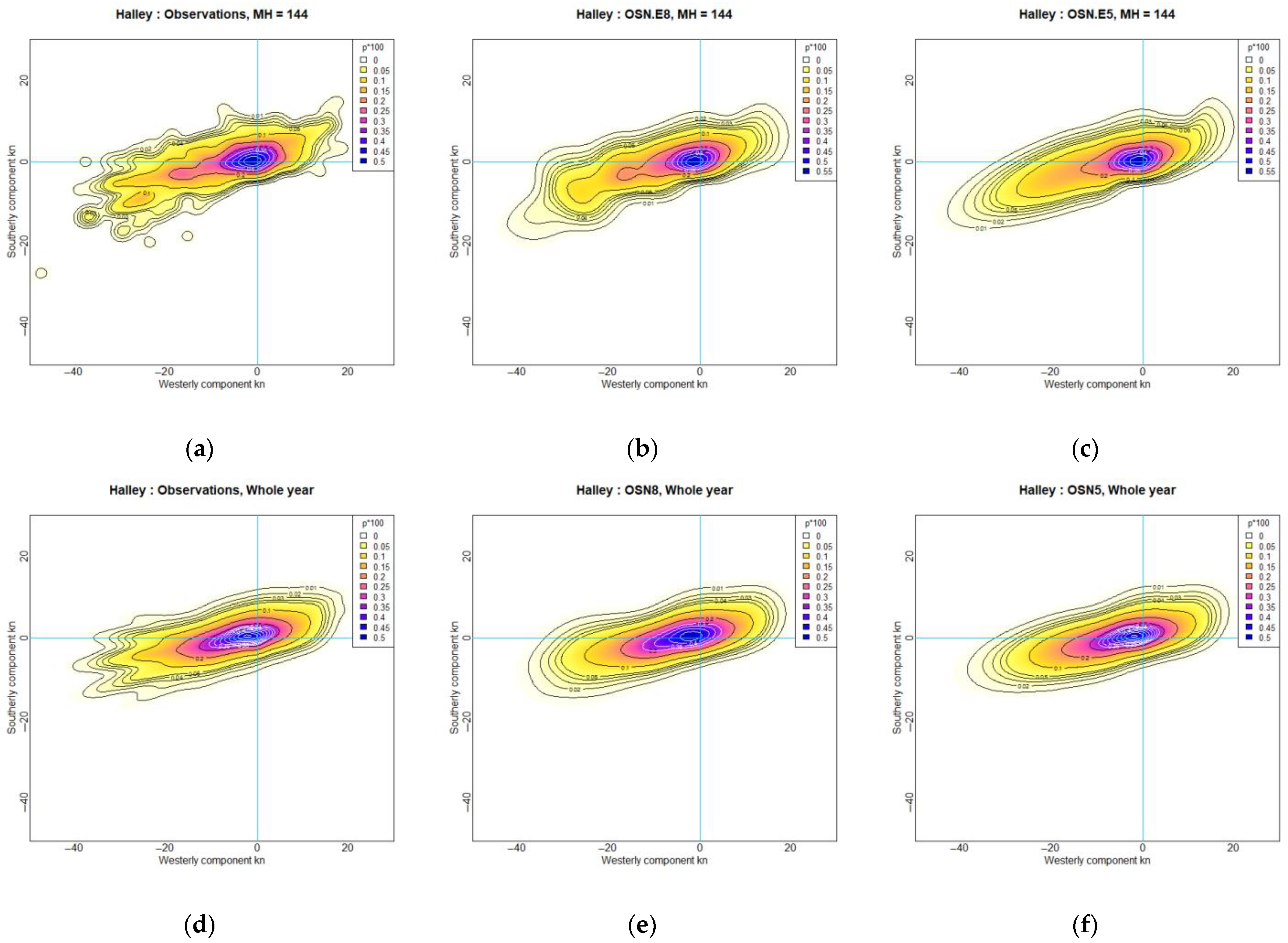
4.2.1. Halley Station

Identified from Figure 13k,l as katabatic, the set of OSN ellipses (3, 5, 6, 8) is strongly skewed on the principal axis, as illustrated in midwinter (July at 00:00) by Figure 15a. The principal axis does not quite intersect with the origin, indicating a southerly drift of about 2 kn, suggesting that the shallow katabatic flow is advected by the overlying polar vortex. The OSN parameters for the merged ellipse were evaluated by rotating the jPDF, $p_{ws}$, into Harris coordinates, $p_{uv}$, integrating for the first three moments of each orthogonal vector, then mapping ${\lambda }_u$ and ${\lambda }_v$from the skew values. (Skewness is mapped from $\lambda$ by integrating for the skew normal distribution moments, and $\lambda$ from skewness by optimization. The mapping functions are included in the R scripts).

The merged ellipse, together with the remaining ellipses (1, 2, 4, 7), formed the initial parameters for refitting as a five-ellipse OSN model. The merged ellipse in Figure 15b is strongly skewed, which is why the merging of katabatic components should be confined to the OSN model. Although the merged components now present as ovoid, it remains convenient to continue calling this an “ellipse”.

This merging process for Halley provides the opportunity to explore how the XOEN models dilute the statistical variance of the observations. In Figure 16, the top row (a–c) corresponds to the single observation time of 00:00 in July (midwinter), while the bottom row (d–f) corresponds to the average over all MH.

At the single MH = 144 (July at 00:00):

(a) 

Owing to the paucity of values and the increasing coarseness of the 10° sectors at higher speeds, $p_{ws}$ presents with ragged contours in the lower-left quadrant, corresponding to the katabatic components. The small, isolated contours represent single observations.

(b) 

The eight-ellipse OSN averages these ragged contours, reducing the spread in this region.

(c) 

The five-ellipse OSN constrains the katabatic component into a single skew normal distribution and allows the other components to adjust accordingly.

Averaging all MH over the whole year:

(d) 

With 228 times more values, the contours resolve the 10° sectors of wind direction.

(e) 

The eight-ellipse OSN averages the whole year sector contours, reducing their spread.

(f) 

The five-ellipse OSN acts as in (c), above.

The cumulative effect of merging the katabatic ellipses at Halley is shown in Figure 17 for the marginal distribution of wind speed, $p\left(V\right)$, where ellipses (3, 5, 6, 8) in (a) merge into ellipse 1 of (b). The eight-ellipse fit is very good for 3 OM, but the five-ellipse fit slightly underestimates in the range 35 to 45 kn. Note that the secondary mode for ellipse 1 in (a) and 3 in (b) is caused by a single outlier at MH = 216 (12:00 in May) (See Section 5.5).

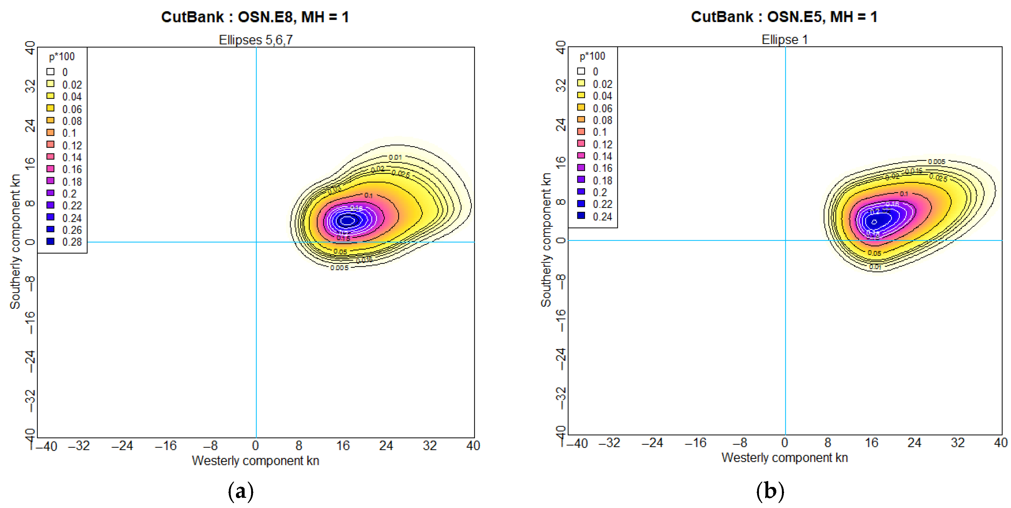
4.2.2. Cut Bank

The same rationalization performed on the katabatic ellipses (5, 6, 7) at Cut Bank is reported in Figure 18 for the merged ellipses and Figure 19 for all ellipses, complementary to Figure 15 and Figure 16 for Halley. The seasonal–diurnal variation at Cut Bank makes the wind climate more complex, but the katabatic winds in winter are comparable in strength to those at Halley. The hodographs in Figure 13i,j suggest that ellipse 7 mostly represents Chinook winds in winter but combines with ellipses 5 and 6 in representing classical cold katabatic winds in summer. Although these are two distinct meteorological mechanisms, their observed characteristics are too alike to be separated definitively.

4.2.3. Summary

While merging the katabatic components into single OSN ellipses appears to compensate for the coarseness of the 10° sectors at higher wind speeds, it comes with the apparent penalty of the slightly poorer GOF metrics in

Table 1. Goodness-of-fit metrics for Halley Station and Cut Bank with katabatic ellipses merged.

	Halley
	OEN.E8	OSN.E8	OSN.E5 *
R2	0.9870	0.9900	0.9818
RMSE	3.62 × 10−5	3.18 × 10−5	4.30 × 10−5
	Cut Bank
	OEN.E8	OSN.E8	OSN.E6 *
R2	0.9950	0.9961	0.9943
RMSE	2.60 × 10−5	2.27 × 10−5	2.78 × 10−5

* With katabatic ellipses merged.

. However, much of the apparent increase in RMSE corresponds to direction-resolution variance, which the OSN ellipses eliminate, i.e., it is observational variance rather than model error. Figure 20 presents the corresponding seasonal–diurnal charts of marginal wind speed and direction distributions at Halley for comparison with Figure 14b, which remains a good match. The effects on other parameters are included in Supplementary Materials for Halley and Cut Bank.

4.3. Merging Split Ellipses

As noted in Section 4.1, splitting is expected in the dominant components, i.e., ellipses with a low rank index, and the two ellipses will lie close together in the hodograph. When split, the relative frequency of the component, $f$, is shared between the two ellipses: $f=f_1+f_2$. Hence, the correlation coefficient of their seasonal–diurnal variation, $\rho (f_1,f_2)$, will be strongly negative. The correlation matrix for $f$ is a useful indicator of ellipses that could be merged. Some meteorological components, particularly land and sea breezes, are negatively correlated by their nature, so, to avoid misidentification, the correlation matrix for the mean speed vector magnitude, $\left|\mathbf{V}\right|={({\overline{W}}^2+{\overline{S}}^2)}^{0.5}={({\overline{U}}^2+{\overline{V}}^2)}^{0.5}$, should also be considered. Land and sea breezes should be negatively correlated for both $f$ and $\left|\mathbf{V}\right|$, whereas split ellipses should be negatively correlated for $f$ and positively correlated for $\left|\mathbf{V}\right|$.

Applying this to the example of Salina,

Table 2. Correlation matrices for $f~\left|\mathbf{V}\right|$ at Salina: Frequencies in upper-right; Mean vectors in lower-left.

	f.1	f.2	f.3	f.4	f.5	f.6	f.7	f.8
$\left|\mathbf{V}\right|$.1	1	−0.63	−0.23	−0.13	0.23	−0.33	0.1	−0.11	f.1
$\left|\mathbf{V}\right|$.2	0.59	1	−0.09	0.18	−0.26	0.1	−0.17	−0.14	f.2
$\left|\mathbf{V}\right|$.3	0.18	0.26	1	−0.26	−0.12	−0.09	−0.47	−0.15	f.3
$\left|\mathbf{V}\right|$.4	−0.3	−0.3	0.35	1	−0.01	0.23	−0.16	0.17	f.4
$\left|\mathbf{V}\right|$.5	0.54	0.73	0.24	−0.1	1	−0.21	−0.17	−0.06	f.5
$\left|\mathbf{V}\right|$.6	−0.2	−0.2	0.26	0.51	−0.2	1	−0.28	0.26	f.6
$\left|\mathbf{V}\right|$.7	−0.1	−0	0.51	0.5	−0	0.48	1	0	f.7
$\left|\mathbf{V}\right|$.8	0.31	0.53	0.18	−0.1	0.3	0.03	0.29	1	f.8
	$\left|\mathbf{V}\right|$.1	$\left|\mathbf{V}\right|$.2	$\left|\mathbf{V}\right|$.3	$\left|\mathbf{V}\right|$.4	$\left|\mathbf{V}\right|$.5	$\left|\mathbf{V}\right|$.6	$\left|\mathbf{V}\right|$.7	$\left|\mathbf{V}\right|$.8

Merger candidates are highlighted in yellow.

presents the correlation matrices of $f$ and $\left|\mathbf{V}\right|$ as upper and lower triangular matrices, respectively. With no precedent to indicate the required degree of correlation, here, a magnitude >0.5 has been assumed, i.e., more likely than not indicating the ellipse pairs (1, 2) and (3, 7) as candidates for merging. These involve the three lowest ranks, and the ellipses of each pair lie alongside each other in the hodographs, as seen in Figure 13a,b. These were merged and refitted in turn, starting with the higher-correlated pair.

Table 3. Goodness-of-fit metrics for Salina.

	Salina
	OEN.E8	OSN.E8	OSN.E7 *	OSN.E6 **
R2	0.9859	0.9888	0.9870	0.9832
RMSE	5.75 × 10−5	5.11 × 10−5	5.45 × 10−5	6.408 × 10−5

* Merging (1,2). ** Merging (1,2) and (3,7).

lists the resulting GOF metrics, where it is seen that each merger results in a small decrease in GOF, but the GOF remains better than the OEN fit after the first merger of (1, 2). The effects on other results are included in the marginal PDFs charts of Figure S17a for the initial OSN.E8, Figure S17b after merging (1, 2) into OSN.E7 and Figure S17c after also merging (3, 7) into OSN.E6—being visually virtually identical.

4.4. Culling Redundant Ellipses

As revealed in [4], individual ellipses can become redundant, i.e., have an insignificant effect on the jPDF, in several ways:

1.

Relative frequency, $f$, approaches zero—the primary effect.

2.

Ellipse centers, the mean vectors, $(U, V),$ migrate outside the computed range.

3.

Standard deviations of the random components, $({\sigma }_u,{\sigma }_v)$, become very large, spreading their contribution thinly over the computed range.

4.

The ellipticity, ${\sigma }_u/{\sigma }_v$, approaches zero or becomes very large, confining their contribution to a thin stripe.

These ways often act in concert, since the second, third and fourth ways are consequences of the primary effect, $f\to 0$, as a paucity of observations makes ellipses more difficult to resolve.

Most redundant ellipses are automatically culled and the XOEN models refitted when their parameters breach the out-of-bound thresholds (Section 2.4.1). The most egregious culls resulted in an improved refit but, typically, the effect on GOF was minimal. However, ellipses can also become redundant by a combination of parameters that individually remain within the thresholds. Two approaches are practical: (a) identify and remove ellipses that are occasionally redundant; and (b) identify and erase ellipses that are always redundant, then refit the model.

A new approach to quantifying “occasional redundancy” was devised to address this issue by evaluating the maximum value of ${\rho }_{ws}$ contributed by each individual ellipse as a ratio of the maximum contribution of all ellipses. This ratio is non-dimensional in the range 0→1 and expresses the relative importance of each ellipse. Hence, redundant ellipses can be selected using a consistent dimensionless threshold, such as 0.005 (½%), which does not differ between locations. This tends to select ellipses with small $f$ and large $({\sigma }_u,{\sigma }_v)$, i.e., those spread thinly across the range. Refitting the remaining ellipses tends to improve GOF marginally. The total number of ellipses remains the same, but these redundant ellipses are inactive with $f=0$. An R script to implement this procedure is provided in the SM as XOEN.CULL.R.

An ellipse is always redundant if the goodness-of-fit improves when it is removed. This may seem counter-intuitive but occurs when the fit to be culled corresponds to a different and better solution than would have been found by fitting the lower number of ellipses directly, as in Figure 7. An R script to implement this procedure for OSN is provided in the SM as XOEN.EraseE.R. This script works for both OEN and OSN models, but the OSN model is better able to compensate for the lost ellipse.

The strategy of sequentially removing the ellipse with the smallest relative frequency until GOF worsens is explored for Fiumicino in

Table 4. Goodness-of-fit metrics for Fiumicino.

	Fiumicino
	OEN.E8	OSN.E8	OSN.E7 *	OSN.E6 **
R2	0.9880	0.9893	0.9902	0.9887
RMSE	9.32 × 10−5	8.71 × 10−5	8.24 × 10−5	8.94 × 10−5

* Removing (8) of OSN.E8. ** Removing (7) of OSN.E7.

. Moving from the eight-ellipse OEN model to the OSN model improves GOF. Reducing to seven ellipses by removing the eighth ellipse improves GOF again, but reducing to six ellipses is worse. The effects on the marginal PDFs are shown in Figure S112.

5. Discussion

5.1. Aims of the Study

This study focused on three principal aims:

1.

Upgrading the OEN model of [4] from supervised automation into unsupervised automation in all aspects, apart from the selection of suitable observational data.

2.

Developing the OSN model to account for observed skewness in components that are directionally constrained.

3.

Demonstrating that the methodology works well in a variety of wind climates and topographic constraints and providing the open-source implementation scripts.

Due to the study’s evolutionary nature, as reflected in the structure of this paper, much of the necessary discussion has already been presented in the earlier sections. Hence, the remainder of Section 5 is confined to emphasizing or expanding on a few key points.

5.2. ”Top Down” Approach to Fitting Ellipses

The earlier methodology [4] added and threaded new ellipses sequentially, suggesting that any target GOF could be reached with a sufficient number of ellipses. Figure 7 shows that not to be true, in that an incremental improvement in GOF eventually reverses and a target GOF might not be reachable. The new methodology is a “top down” approach in which multiple ellipses are fitted in parallel; then, the number of ellipses is reduced by finding and culling unstable and redundant ellipses. This reduces the computational overhead by two orders of magnitude (OM), from several days to a few hours, but requires at least 12 processor cores to enable parallel processing. It also eliminates any possibility of observer bias in the model fitting, as the results emerge warts-and-all because supervision is confined to the initial selection of suitable observational data and to post-fitting actions, such as merging ellipses and resolving outliers. Although the rationalization of the ellipses was manually supervised in this study, the reasoning employed in identifying candidates points to strategies for future unsupervised automation.

5.3. Threading

The new fully automated threading ensures continuity in the diurnal variation within each month. Continuity is maintained between months when the seasonal variation is gradual, but not for all ellipses when sudden changes occur close to a change of month and there is no continuity of pattern to support the threading. Monsoon climates jump suddenly between metastable “summer” and “winter” states, resulting in two distinct sets of ellipses that share the threads. Whereas the manual supervision of the threading process of [4] can lead to unique threads with a 1:1 correspondence with the physical meteorology [2,3], the revised methodology prioritizes the minimization of RMSE and splits components into multiple ellipses if this furthers that aim. When physical meteorology is irrelevant to an application, consistent threading is of little importance because the overall statistical properties are unaffected, but it does serve to produce neater charts for the study report, e.g., Figure 9.

5.4. Residual Error

The residual error of each model, indicated by the overall RMSE, includes the statistical variance of the observations that are diluted by the model and dependent on the quality of the observations. Given that the observational variance has a fixed value in each data set, the reduction in RMSE in Figure 7b from fitting 4 ellipses to the minimum value at around 11 ellipses can be attributed to reduction in model error, with the minimum value representing the observational variance.

Little improvement in RMSE is gained by using more than eight ellipses in the initial OEN fit. Adopting the OSN model quadruples the fitting time for a marginal gain. Merging katabatic ellipses (Section 4.2) and split ellipses (Section 4.3) are neutral. Therefore, it is a moot point whether the additional overheads of these additional actions are necessary in many practical applications, especially when the application requires integral statistics, e.g., in estimating wind energy potential. The unsupervised culling of redundant ellipses and refitting in Section 4.4, which produces a marginal improvement in GOF, is recommended to remove redundant ellipses and retain only the essential set for each MH.

5.5. Outlier Fits

The automated unsupervised analysis process has been reported “warts-and-all” to prove the efficacy of the methodology by using observations from stations that provide an onerous test. The outlier in $p\left(V\right)$ for ellipse 1 for MH = 216 at Halley, Figure 17a, as noted in Section 4.2.1, is one of the few occasional “warts” that were revealed. This cause is examined in Figure 21 where it is seen that one of the isolated contours has sufficient influence to define a new ellipse 8, reducing the number of ellipses defining the body of the distribution. The former ellipses 1 and 2 merge and ellipse 1 takes the former position of 8, which is why the secondary mode of ellipse 1 and the mode of ellipse 8 are aligned in Figure 19a. This anomaly was corrected by re-initialization using the correctly threaded neighbor MH = 217 and refitting. It is remarkable that this is the only obvious “wart” to emerge in 4032 fits and speaks to the robustness of the OEN/OSN fitting and threading process. Strategies for unsupervised detection and the correction of outlier fits are being developed and will be incorporated in any future update of the R scripts. For now, charts of $p\left(V\right)$ for the individual ellipses are convenient indicators of suspected outliers.

5.6. The Fuzzy Demodulation

The fuzzy demodulation of [4] was used in Section 2.5 to explore the apparent deviations from normal and excess kurtosis of the orthogonal vectors it produces. Independent assessment through fitting the SGT model confirms that excess kurtosis remains effectively zero, and that the deviations are an artefact manufactured by the process. So far, the fuzzy demodulation process of [4] remains the only viable route to the autocorrelations of the orthogonal vectors, thence to the spectra and integral timescales. This study indicates that values outside a threshold, set by reference to the fuzzy PDF, should be discarded when evaluating the autocorrelations. In the case of Tokyo, Figure 10, this threshold would be $~4\sigma$ for ellipse 1 and $~3\sigma$ for ellipse 8, corresponding to 3–2 OM (0.1–1%) on $p_{ws}$. The fuzzy demodulation is also the only route to assessing the duration each component is active or inactive, which is a necessary first step in the quest to generate realistic long-duration timeseries simulations and a subject for future studies.

5.7. Annual Marginal Distributions of Wind Speed and Direction

The annual marginal distribution of wind speed and direction, $p\left(V\right)$ and $p\left(\theta \right)$, are principal metrics in studies where seasonal/diurnal variation is of no interest. These may be evaluated from the XOEN models and are included in the Supplementary Figures for each of the eight locations of this study. Here, they are presented together in Figure 22 and Figure 23 to facilitate comparison between the study stations. These charts compare the observed $p\left(V\right)$ and $p\left(\theta \right)$ with those evaluated from OSN and show the contributions of each ellipse to the model.

Speed distributions, $p\left(V\right)$, in Figure 22 show consistent good fit over 2–3 OM (1–0.1%), matching the acceptable range of the fuzzy demodulation. Observations further into the far tail contribute little to the model fit and are less reliable, so the model may lie above or below the observations, depending on the component ellipses that dominate the far tail. Better fit further into the tails could be achieved by minimizing the error in $\mathrm{l}\mathrm{n}\left(p_{ws}\right)$, giving the tail more weight, but at the expense of a poorer fit in the body of the distributions. The chart for Halley shows the outlier-corrected version of Figure 19a.

Direction distributions, $p\left(\theta \right)$, in Figure 23 show a reasonable fit of the OSN model to the observations, except when passing through $\theta =0°.$In most cases, the observations appear discontinuous through $\theta =0°$, suggesting there may be issues with the way that the ten-minute mean of the observed wind direction is measured over the break in value. The observed FM12/FM15 wind direction is the ten-minute mean of the argument of the wind vector, $\overline{(\angle \mathbf{V})}$, as measured by a vane, but this causes issues when averaged over the break in value between $\theta =360°$ and $\theta =0°$. This is not concommitant with the argument of the ten-minute mean vector,$\mathbf{\angle }\overline{\mathbf{V}}$, provided by the XOEN model since, due to the non-linear relationship, $\overline{(\angle \mathbf{V})}\ne \mathbf{\angle }\overline{\mathbf{V}}$. On the other hand, the model evaluation is continuous through 0°, obviating any need to employ empirical polar distributions such as von Mises [32,33].

References

- Harris, R.I.; Cook, N.J. The Parent Wind Speed Distribution: Why Weibull? J. Wind Eng. Ind. Aerodyn. 2014, 131, 72–87. [Google Scholar] [CrossRef]
- Cook, N.J. A Statistical Model of the Seasonal-Diurnal Wind Climate at Adelaide. Aust. Meteorol. Oceanogr. J. 2015, 65, 206–232. [Google Scholar] [CrossRef]
- Cook, N.J. Parameterizing the Seasonal–Diurnal Wind Climate of Rome: Fiumicino and Ciampino. Meteorol. Appl. 2020, 27, e1848. [Google Scholar] [CrossRef]
- Cook, N.J. Automated Probabilistic Analysis and Parametric Modelling of the Seasonal-Diurnal Wind Vector. J. Energy Power Technol. 2021, 3, 027. [Google Scholar] [CrossRef]
- Brooks, C.E.P.; Durst, C.S.; Carruthers, N. Upper Winds over the World: Part I. The Frequency Distribution of Winds at a Point in the Free Air. Q.J R. Met. Soc. 1946, 72, 55–73. [Google Scholar] [CrossRef]
- Crutcher, H.L. On the Standard Vector-Deviation Wind Rose. J. Meteorol. 1957, 14, 28–33. [Google Scholar] [CrossRef]
- Crutcher, H.L.; Baer, L. Computations from Elliptical Wind Distribution Statistics. J. Appl. Meteor. 1962, 1, 522–530. [Google Scholar] [CrossRef]
- Crutcher, H.L.; Joiner, R.L. Separation of Mixed Data Sets into Homogeneous Sets; NOAA Technical Report; National Climatic Center: Asheville, NC, USA, 1977; p. 167. [Google Scholar]
- Crutcher, H.L.; Joiner, R.L. Another Look at the Upper Winds of the Tropics. J. Appl. Meteor. 1977, 16, 462–476. [Google Scholar] [CrossRef]
- Cramér, H. Mathematical Methods of Statistics (PMS-9); Princeton Mathematical Series; Princeton University Press: Princeton, NJ, USA, 2016; ISBN 978-0-691-00547-8. [Google Scholar]
- Chen, Q.; Yu, C.; Li, Y. General Strategies for Modeling Joint Probability Density Function of Wind Speed, Wind Direction and Wind Attack Angle. J. Wind Eng. Ind. Aerodyn. 2022, 225, 104985. [Google Scholar] [CrossRef]
- Wang, H.; Xiao, T.; Gou, H.; Pu, Q.; Bao, Y. Joint Distribution of Wind Speed and Direction over Complex Terrains Based on Nonparametric Copula Models. J. Wind Eng. Ind. Aerodyn. 2023, 241, 105509. [Google Scholar] [CrossRef]
- Wang, Y.; Li, Y.; Zou, R.; Song, D. Bayesian Infinite Mixture Models for Wind Speed Distribution Estimation. Energy Convers. Manag. 2021, 236, 113946. [Google Scholar] [CrossRef]
- Cook, N.J. Detecting Artefacts in Analyses of Extreme Wind Speeds. Wind Struct. 2014, 19, 271–294. [Google Scholar] [CrossRef]
- WMO. Guide to Meteorological Instruments and Methods of Observation, Volume I: Measurement of Meteorological Variables, 2021st ed.; World Meteorological Organization: Geneva, Switzerland, 2021; ISBN 978-92-63-10008-5.
- Takle, E.S.; Brown, J.M. Note on the Use of Weibull Statistics to Characterize Wind-Speed Data. J. Appl. Meteor. 1978, 17, 556–559. [Google Scholar] [CrossRef]
- Lee, S.X.; McLachlan, G.J. An Overview of Skew Distributions in Model-Based Clustering. J. Multivar. Anal. 2022, 188, 104853. [Google Scholar] [CrossRef]
- Haurwitz, B. Comments on the Sea-Breeze Circulation. J. Meteor. 1947, 4, 1–8. [Google Scholar] [CrossRef]
- Staley, D.O. The Low-Level Sea Breeze of Northwest Washington. J. Meteor. 1957, 14, 458–470. [Google Scholar] [CrossRef]
- McCaffery, W.D.S. On Sea-Breeze Forecasting Techniques; Forecasting Techniques Branch Memorandum; Meteorological Office: Exeter, UK, 1966; p. 43. [Google Scholar]
- Reed, J.W. Cape Canaveral Sea Breezes. J. Appl. Meteor. 1979, 18, 231–235. [Google Scholar] [CrossRef]
- Staley, D.O. The Surface Sea Breeze: Applicability of Haurwitz-Type Theory. J. Appl. Meteor. 1989, 28, 137–145. [Google Scholar] [CrossRef]
- Moisseeva, N.; Steyn, D.G. Dynamical Analysis of Sea-Breeze Hodograph Rotation in Sardinia. Atmos. Chem. Phys. 2014, 14, 13471–13481. [Google Scholar] [CrossRef]
- Furberg, M.; Steyn, D.G.; Baldi, M. The Climatology of Sea Breezes on Sardinia. Int. J. Climatol. 2002, 22, 917–932. [Google Scholar] [CrossRef]
- Kusuda, M.; Alpert, P. Anti-Clockwise Rotation of the Wind Hodograph. Part I: Theoretical Study. J. Atmos. Sci. 1983, 40, 487–499. [Google Scholar] [CrossRef]
- Cook, N.J. Extreme Convective Gusts in the Contiguous USA. Meteorology 2024, 3, 281–309. [Google Scholar] [CrossRef]
- Physick, W.L.; Byron-Scott, R.A.D. Observations of the Sea Breeze in the Vicinity of a Gulf. Weather 1977, 32, 373–381. [Google Scholar] [CrossRef]
- Grace, W.; Holton, I. Hydraulic Jump Signatures Associated with Adelaide Downslope Winds. Aust. Meteorol. Oceanogr. J. 1990, 38, 43–52. [Google Scholar]
- Tepper, G.; Watson, A. The Wintertime Nocturnal Northeasterly Wind of Adelaide, South Australia: An Example of Topographic Blocking in a Stably-Stratified Air Mass. Aust. Meteorol. Oceanogr. J. 1990, 38, 281–291. [Google Scholar]
- Sha, W.; Grace, W.; Physick, W. A Numerical Experiment on the Adelaide Gully Wind of South Australia. Aust. Meteorol. Oceanogr. J. 1996, 45, 19–40. [Google Scholar] [CrossRef]
- Cook, N.J. Visualising Seasonal-Diurnal Trends in Wind Observations. Weather 2015, 70, 117–121. [Google Scholar] [CrossRef]
- Carta, J.A.; Ramírez, P.; Bueno, C. A Joint Probability Density Function of Wind Speed and Direction for Wind Energy Analysis. Energy Convers. Manag. 2008, 49, 1309–1320. [Google Scholar] [CrossRef]
- Han, Q.; Hao, Z.; Hu, T.; Chu, F. Non-Parametric Models for Joint Probabilistic Distributions of Wind Speed and Direction Data. Renew. Energy 2018, 126, 1032–1042. [Google Scholar] [CrossRef]