Article

Performance Rank Variation Score (PRVS) to Measure Variation in Ensemble Member’s Relative Performance with Introduction to “Transformed Ensemble” Post-Processing Method

Environmental Modeling Center, National Centers for Environmental Prediction, National Oceanic and Atmospheric Administration, College Park, MD 20740, USA
Meteorology 2025, 4(3), 20; https://doi.org/10.3390/meteorology4030020
Submission received: 16 April 2025 / Revised: 3 July 2025 / Accepted: 21 July 2025 / Published: 25 July 2025

Abstract

In an ensemble prediction system, each member performs differently from each other for individual cases. To adaptively (not only statistically) calibrate or post-process raw ensemble forecasts and produce more reliable and accurate forecast products case by case, it is necessary to understand how individual ensemble members behave inside an ensemble cloud. For example, how (randomly or orderly) does an individual member’s relative performance (including the best and worst members) vary with location and time? To quantify and understand these variations, this study proposes the “Performance Rank Variation Score (PRVS)” to measure the degree of ensemble member’s relative performance variation (the “motion” of members). The PRVS was applied to four real cases (representing the winter, spring, summer, and fall seasons) from the NCEP global ensemble forecast system (GEFS). Many interesting results were observed, which are otherwise hard to elucidate without this new score. At the same time, based on the revealed results, possible ensemble post-processing strategies are discussed for future developments, where a new concept of “transformed ensemble” was demonstrated as an example.

1. Introduction

Dealing with the predictability issue of atmospheric motion (Lorenz, 1963 [1], 1965 [2], 1993 [3]; Thompson, 1957 [4]), an ensemble prediction system (EPS, Du et al., 2018 [5]) is a major component of the operational numerical weather prediction (NWP) model suite at many NWP centers around the world (Buizza et al., 2018 [6]; Toth and Kalnay, 1993 [7]; Molteni et al., 1996 [8]; Houtekamer et al., 1996 [9]; Du et al., 1997 [10]; and Chen et al., 2025 [11]). An EPS provides multiple forecasts or ensemble members at the same time. Although each ensemble member should perform equally on average in many cases for a well-behaved EPS (such as perturbing initial condition only), each member performs differently for individual cases, as well as at a given location and forecast time. Those differences could be very large depending on the situation. In real-world applications, it is the individual case that matters (not the average statistics). It is those individual cases that need to be calibrated by post-processing methods to improve day-to-day real-time weather forecasts. To adaptively (not only statistically) calibrate or post-process raw ensemble forecasts and produce more reliable and accurate forecast products case by case, it is necessary to understand how individual ensemble members behave inside an ensemble cloud. For example, how (randomly or orderly) does an individual ensemble member’s relative performance (including the best and worst members) vary with location and time? To the author’s knowledge, there is no such measurement that exists yet. To quantify and understand these variations, this study proposes the “Performance Rank Variation Score (PRVS)”, which measures the degree of an ensemble member’s relative performance variation (the “motion” of members) within an ensemble. The PRVS was applied to four real cases (representing the winter, spring, summer, and fall seasons) from the NCEP global ensemble forecast system (GEFS, Zhou et al. [12], 2022; Fu et al., 2024 [13]). Many interesting results were observed, which are otherwise hard to elucidate without this new score. At the same time, based on the revealed results, possible ensemble post-processing strategies are discussed for future developments, where a new concept of “transformed ensemble” was demonstrated in particular.
The current version (version 12) of operational GEFS is based on the NCEP global forecast system (GFS), an FV3 dynamic core-based model (Lin et al., 2017 [14]). It has 31 members (1 unperturbed control forecast and 30 perturbed members) in about a 25 km horizontal resolution with a forecast length of 35 days (840 h), and outputs every six hours. It runs four cycles per day at 00, 06, 12, and 18 z. The initial condition perturbation is provided by the ensemble Kaman filter (EnKF, Houtekamer and Mitchell, 1998 [15])-based data assimilation system (Kleist and Ide, 2015 [16]). Stochastic physics is used to address physics uncertainty. Four forecast cases from 2024, representing winter (27 February), spring (1 May), summer (1 July 2024), and fall (1 October), were tested with the new score. Since the results are very stable and similar for the four cases, only the winter case is presented in detail, while the average result of the four cases is presented by two summary figures at the end. To see more detailed spatial structures, our application was performed on an interpolated 3 km Continental United States domain (CONUS, 1799 × 1059 = 1,905,141 grid points). The first 16 days (384 h) of forecasts were examined.
This paper is organized as follows: following the introduction (Section 1), the PRVS is defined and explained in Section 2.1. An application of the new score to the real GEFS cases is demonstrated in Section 2.2. Section 3 discusses possible effective ensemble post-processing strategies based on the revealed results, where a new concept of “transformed ensemble” is presented. A summary is given in Section 4.

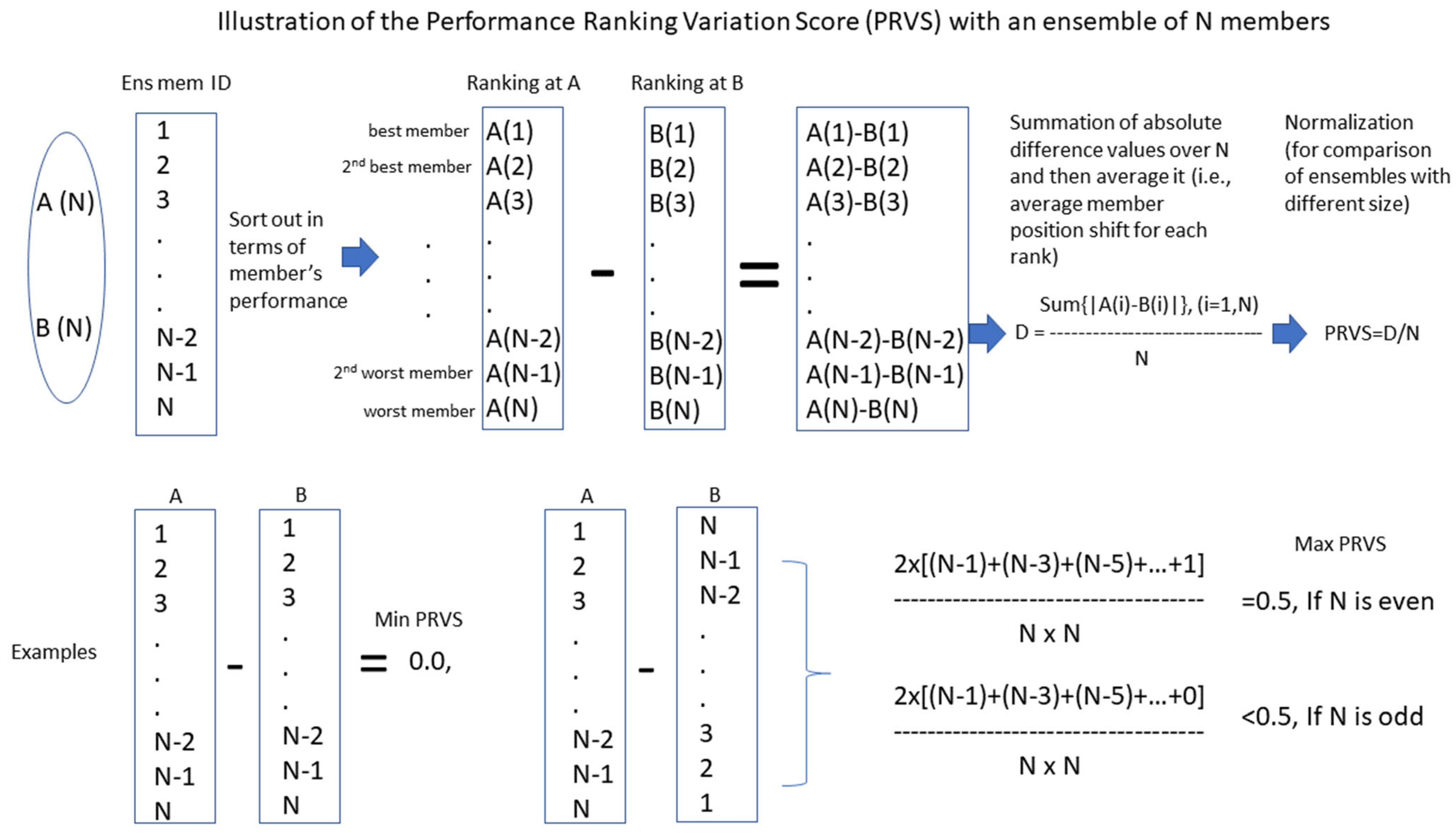
2. Performance Rank Variation Score (PRVS)

2.1. Definition

The Performance Rank Variation Score (PRVS) is illustrated and explained in detail in Figure 1. Mathematically, assuming there are N members in an ensemble, the PRVS between Point A and Point B can be defined and calculated as follows:
P R V S = 1 N × N i = 1 N A i B i
where A(i) and B(i) are member identity (ID = 1, 2, 3, …, N − 2, N − 1, N) arrays of the performance ranking (e.g., ranging in order from the best to the worst member or the other way around) at Point A and Point B, respectively. The performance measure can be anything defined by a researcher to meet their specific goal of study. The absolute forecast error (|forecast − analysis|) is used to measure performance in this study. For example, the member performance ranking is (2, 3, 1) at A and (3, 1, 2) at B for a three-member ensemble, where the member performance can be measured by their forecast errors (e.g., absolute forecast error). The absolute values of the difference |A(i) − B(i)| are summed up over all N ranks, which is first averaged over N ranks and then normalized by ensemble size N for generality (for comparability of different size ensembles). For this three-member ensemble, P R V S = 1 3 × 3 ( 2 3 + 3 1 + 1 2 ) = 1 3 × 3 4 = 0.444 . The PRVS varies from 0.0 to 0.5 depending on if N is an even or odd value (see Figure 1), representing an average variation (or shift) in each rank. For example, if PRVS = 0.323 for an N = 31 ensemble, it means that the member ID difference or shift is, on average, about 10 positions (0.323 × 31 = 10) for each rank. If the fifth best performer is member #15 at Point A, the member ID of the fifth best performer at Point B might be member #5 or member #25. The PRVS can also be applied to a particular rank i t h   (i.e., one rank instead of N ranks), and Equation (1) can then be simplified to
P R V S i = 1 N A i B i
The value of P R V S   i can vary from 0.0 to N 1 N for a single rank. Assuming that the performance rank order is arranged from the best (first) to the worst (Nth), then the PRVS for the best and worst members can be expressed by Equations (3) and (4), respectively.
P R V S b e s t = P R V S 1 = 1 N A 1 B 1
P R V S w o r s t = P R V S N = 1 N A N B N .

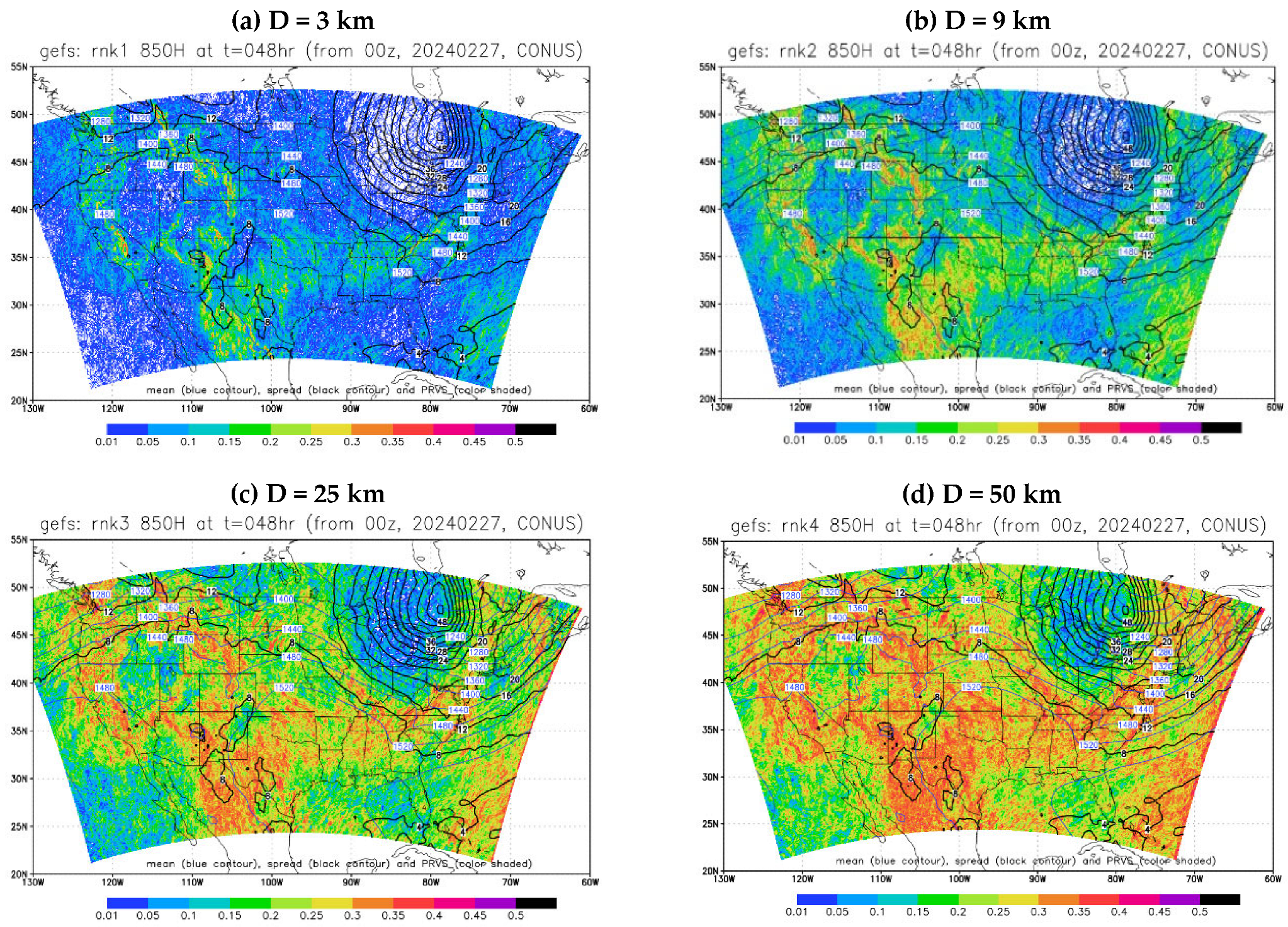
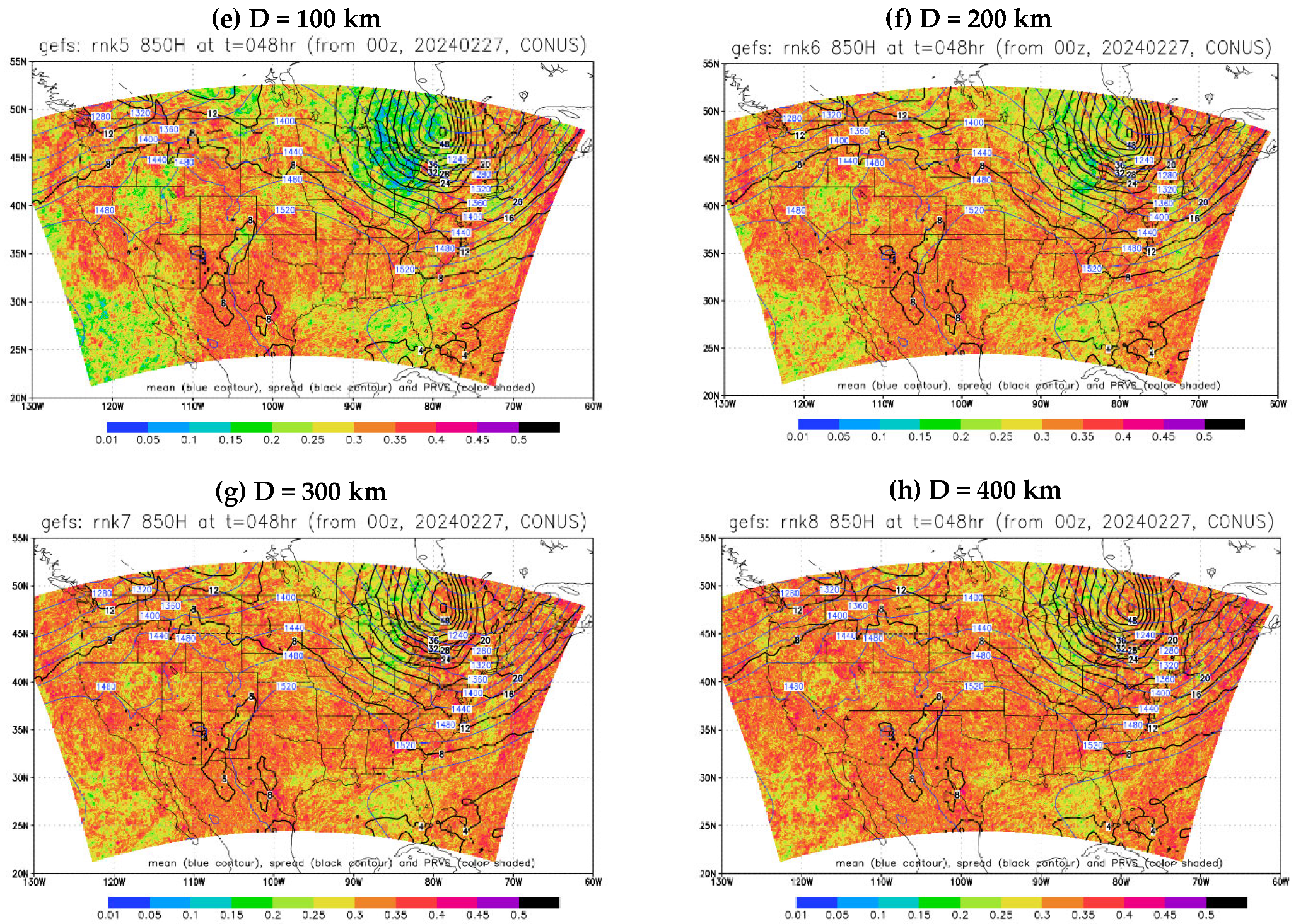
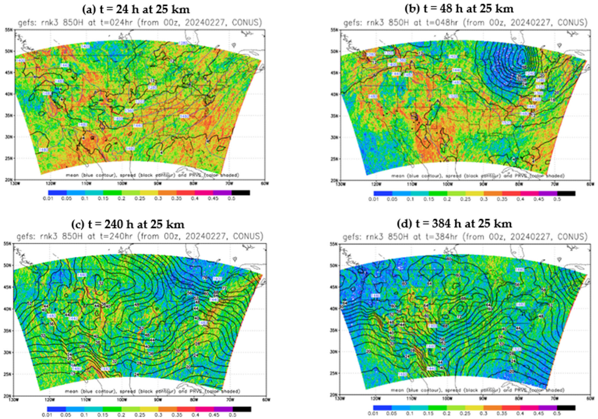
2.2. Application in GEFS Forecasts

Figure 2 shows an example of the PRVS at each grid point from the 48 h 31-member GEFS forecast of 850H (initiated from 00z, 27 February 2024), calculated between a grid point and another neighboring grid point separated by different distances (D = 3, 9, 25, 50, 100, 200, 300, and 400 km approximately). The PRVS is calculated at every grid point within the verification domain. For each grid point, its neighboring grid point is chosen along the longitudinal direction (to east). The separation distance is based on how many grid points are between them, e.g., 3 km for every grid point, 9 km for every three grid points, 25 km for every eight grid points, and so on, rounded to a value easier to remember such as 50, 100, 200, 300, and 400 km for a 3 km resolution verification grid. Not surprisingly, the PRVS increases rapidly with the increase in the separation distance. However, even at a 3 km separation distance, the PRVS ranges from 0.15 to 0.35 over many areas. This indicates that the member identity order in the member’s performance rank is vastly different from one location to another even if the two locations are not far apart. The variation has nearly reached its maximum if the separation distance exceeds 200–300 km, indicating that the member order of the performance rank at one point could be completely different from that at another point at about 200 km apart and beyond. By comparing the PRVS with the ensemble spread (black contour), we can see that the PRVS tends to be smaller when the spread is larger. This is understandable because when members are separated by larger values (larger spread), a member’s relative rank position will be easier to maintain and more difficult to be switched by other members. Since the PRVS considers only the order of members but not the magnitude of their differences, it will be interesting to study its relationship to forecast predictability or spread (“motion vs. magnitude”) in future studies.
Figure 3 and Figure 4 show the PRVS at different forecast lengths (short, medium, and long range) using two separation distances of 25 km (Figure 3) and 200 km (Figure 4). The PRVS has a noticeable decreasing trend with forecast hours at shorter separation distances (25 km, Figure 3), probably due to the increase in spread with forecast length. However, this decreasing trend is not obvious for the longer separation distance (200 km, Figure 4) probably due to the saturation of the PRVS at separation distances exceeding 200 km, as seen from Figure 2. To quantify what we have observed from Figure 2, Figure 3 and Figure 4, Figure 5 is the domain-averaged PRVS of more variables, which confirms the results of Figure 2, Figure 3 and Figure 4. These are that (a) the PRVS increases with the increase in the separation distances, becoming saturated at 200–300 km, and (b) the PRVS decreases slightly with the increase in forecast length (from day 1 to day 10 to day 16) due to the spread increase, especially at shorter separation distances (e.g., 25 km). Besides these two characteristics, it is also noticed that the membership variation is larger for surface temperature (T2m) and wind (850U) than height (500H) and pressure (SLP) fields because the former (T2m and 850U) is normally less predictable than the latter (500H and SLP).
The PRVS is also calculated for the best (Equation (3)) and worst (Equation (4)) members, and their domain-averaged values are shown in Figure 6a and Figure 6b, respectively. The result of the best member (Figure 6a) is very similar to the average variation in the full member’s performance rank (Figure 5). However, the behavior of the worst member (Figure 6b) is noticeably different from that of the best member (Figure 6a). PRVS_worst is much smaller than PRVS_best, which means that the member identity of the worst member changes much less frequently and remains the same over a larger area, especially over longer time range (like Day 10 and 16). This can be confirmed by Figure 7 and Figure 8.
Figure 7 and Figure 8 show how the member identity of the best performer and worst performer flip around over the domain, respectively. They are constantly changing across space, i.e., the member identity of the best and worst forecasts in one location is different from that at another location. This spatial variation is much more frequent (or on a much smaller spatial scale) for the best member (Figure 7) than the worst member (Figure 8). It implies that there are more members being around the truth and being close to each other, which results in frequent member identity switching for the best member. At the same time, the outliers (i.e., the worst member) that are far away from the truth have far fewer members, which results in much less frequent member identity switching. This fact is the basis of “a dynamical performance-ranking method” proposed by Du and Zhou (2011), with the ensemble mean being closer to the truth. Figure 7 and Figure 8 also show that, for both the best and worst members, the frequency of member identity changing decreases with the increase in forecast length. This decrease is likely due to the spread increase with forecast length, a result that is consistent with the PRVS results (e.g., Figure 3).
Could the variation frequency of the worst member shown in Figure 8 be related to the flow regime? Figure 9 shows the GFS analysis of 850H corresponding, respectively, to days 1, 10, and 16 in Figure 8. Qualitatively, we do see some kind of relationship existing between them. For example, for day 1, the larger variation in the worst member identity over the eastern part of the US (Figure 8a) is coincident with the larger gradient area in front of the trough (Figure 9a). For day 10, the two larger variation areas (central US and northwest US, Figure 8b) are coincident with the two low-pressure systems (Figure 9b). For day 16, the larger variation area over central US (Figure 8c) is coincident with the cyclone over the same region (Figure 9c). However, not all relationships can be explained in such a straightforward way, e.g., the larger variation along the US East Coast (Figure 8c) is associated with a ridge at day 16 (Figure 9c). Therefore, a quantitative study on this relationship will be practically helpful and scientifically insightful. The above results are for the winter case (20240227). To make sure that the results are robust, we performed the same calculations for another three cases (20240501, 20250701, and 20241001) representing the other three seasons (spring, summer, and fall). It is found that the domain-averaged statistical PRVS results are very stable and similar to each other for all four cases, although their detailed spatial patterns could be flow-dependent (see the above discussion related to Figure 8 and Figure 9). The summary results averaged over the four cases are presented in Figure 10 and Figure 11. By comparing Figure 10 with Figure 5 or Figure 11 with Figure 6, all previous conclusions remain the same.

3. Discussion of Possible Ensemble Post-Processing Methods

The large spatial variation in the member identity of the full performance ranking best performers, and worst performers, as revealed in the last section, implies that extracting useful formation simultaneously at all locations out of an ensemble cloud (like putting a puzzle back together) is extremely challenging and nearly impossible. This reminds us of the chaotic nature of the atmosphere and emphasizes that the primary mission of an ensemble forecast should provide a spectrum of probable outcomes of a future weather event rather than a single outcome. At the same time, our results also shed some light on the path forward of ensemble post-processing. For example, it might be easier and more effective to calibrate raw ensemble forecasts at a longer range and target worst members rather than best members because the worst members have smaller member identity variations. In other words, it might be possible to identify and exclude a few persistently worst members to greatly improve ensemble products, especially for an over-dispersive ensemble.
Following this idea, we tested a new ensemble post-processing method called “transformed ensemble”. Since the ensemble mean is generally closer to the truth, we use the ensemble mean as an approximation of truth (Du and Zhou, 2011 [17]). The distance of each member to the ensemble mean (i.e., their absolute difference for a variable of your choice) is calculated to determine outlier members with the largest distances. A few of these extreme outlier members are then discarded. The number of outlier members to be discarded depends on the over-dispersion statistics of the ensemble spread. Unlike the method in Du and Zhou (2011 [17]) where the performance ranking was done by shuffling whole ensemble members (e.g., based on the entire domain-averaged value of a member. Therefore, their method can be called “reshuffled ensemble”), this process is carried out at each grid point individually for each variable to form new transformed ensemble members. Thus, in this newly formed ensemble, their original ensemble identity could be very different among neighboring grid points. To avoid information loss due to the “return to skill” of ensemble members (Bright and Nutter, 2004 [18]), this transforming process is also carried out independently for each forecast hour during the forecast length. The new ensemble can be used in different ways. For example, based on the estimated each member’s performance, a reduced-size ensemble (“transformed ensemble”) can be formed by discarding a few “worst” members. Weighted ensemble mean and probability can also be constructed based on the new ensemble, similar to that of Du and Zhou (2011 [17]). For proof of concept, Figure 12a compares the absolute forecast errors of the worst and best members between the transformed (25 members) and raw ensemble (31 members) for T2m in the above GEFS summer case (20240701), where the worst and best members are ranked independently for each grid point and their errors are then averaged over the verification domain. We can see that the forecast error of the worst member in the transformed ensemble (red solid curve) is indeed greatly reduced compared to the raw ensemble (blue solid curve). The overall accuracy of ensemble members is improved too: the average error of individual members in the transformed ensemble is apparently reduced compared to the raw ensemble (Figure 12b). At the same time, throwing the baby out with the bathwater is a possible caveat. Figure 12a shows that the error of the best member in the transformed ensemble (red dashed curve) is slightly higher than the raw ensemble (blue dashed curve), indicating that some good information is lost. This caveat is certainly related to the size of the raw ensemble and the number of members being discarded. The larger raw ensemble and less members being discarded should minimize the negative effect of the caveat. In this test, six members were discarded out of 31 members, which should result in some level of negative impact. The number of outlier members being discarded needs to be carefully tested depending on the over-dispersion statistics of the ensemble spread to maintain a good reliability of the ensemble. With the increase in ensemble size, especially during the incoming era of artificial intelligence/machine learning (AI/ML) weather forecasting, this caveat might become a non-issue. Given the fact that many EPSs have already shown over-dispersion, especially at longer range, the author argues that it is time to consider discarding bad members rather than adding new members in an ensemble to improve its quality (Du, 2025 [19]). Since ensemble prediction is especially valuable for rare extreme weather events, our next endeavor is to examine how this transformed ensemble method works for extreme weather events and implement rules to avoid incorrectly discarding likely extreme events. As pointed out by the ensemble dynamical performance-ranking method (Du and Zhou, 2011 [17]), model bias will parallel shift each members’ position and incorrectly recognize the outliers with respect to the ensemble mean; bias correction should be performed prior to the application of the transformed ensemble method to reduce the chance of the caveat occurring.
The results of the last section show the spatial variation in ensemble members’ identity in their relative performance ranking for one variable at a forecast time. How are these variations connected among different variables and different forecast times? Figure 13 shows the ensemble performance rank histogram of the same case for four variables (T2m, 500H, 850U, and SLP) at a short range (day 1, Figure 13a), medium range (day 10, Figure 13b), and long range (day 16, Figure 13c). The histogram includes domain-averaged statistics that measure how frequently a member is the closest to the truth (i.e., performance rank) over all grid points within the verification domain out of the 31 GEFS members. It can be seen that each member performs differently from each other. The difference apparently amplifies with the increase in forecast time, which further supports the earlier claim that the ensemble post-processing of raw model forecasts will be made more important and effective by discarding bad members to improve forecast information at longer ranges.
Figure 14a is the cross-variable correlation—the correlation between the performance rank histograms (Figure 13) of two different variables at each forecast time. The cross-variable correlation is generally positive, indicating that different variables are correlated with each other in their relative performance positions. For example, if the mass field performs better, the corresponding wind field is likely to perform better too. This is an encouraging result that makes it possible to use one variable to calibrate other variables in post-processing for physics-based models like GEFS (will an AI or machine learning-based data-driven model preserve this property? The answer is probably a yes, see Du et al. (2025 [20])). However, this cross-variable correlation becomes very weak around day 9, indicating that this relation is flow-dependent. Figure 14b is the cross-time correlation—the correlation between the performance rank histograms of the same variable but at different forecast times for the same four selected variables. At reference forecast hour t, the correlation is calculated between the reference forecast time t and a future forecast time, using intervals of 12 h, e.g., t + 0, t + 12, t + 24, t + 36, and t + 48 … hours. The result is calculated and averaged over the entire forecast length from 12 h to 384 h, as shown in Figure 14b. We can see that the performance rank histograms are positively correlated when the forecast time difference is less than about two days apart, and no correlation is found if the forecast time difference is more than three days apart. This is true for all four variables. The shorter time memory of an ensemble member’s relative performance implies that the potential value of using the performance of an earlier-hour forecast to calibrate a later-hour forecast will be limited, although it might still possible for short-range forecasts like 1–2 days in advance. For example, based on this result, we can anticipate that the ensemble sensitivity-based ensemble subletting approach (Ancell, 2016 [21]) will not work well beyond 2–3 days in real-world practice.

4. Summary

This study has proposed a new measuring score, the “Performance Rank Variation Score (PRVS)”, to measure the variation in ensemble members’ relative performance variation within an ensemble cloud. The PRVS was applied to four cases of NCEP GEFS forecasts representing four reasons (winter, spring, summer, and fall). Given that similar results are seen in all four cases, the winter case is presented in detail and the other three cases are included as summarized result. Many interesting results were observed. Based on the results revealed, possible ensemble post-processing strategies were discussed. In particular, a new concept of “transformed ensemble” is introduced for ensemble post-processing. The PRVS results can be generalized with confidence, while more studies are needed for the details and robustness of the “transformed ensemble” method. Below is what we learned from this study.
(1)
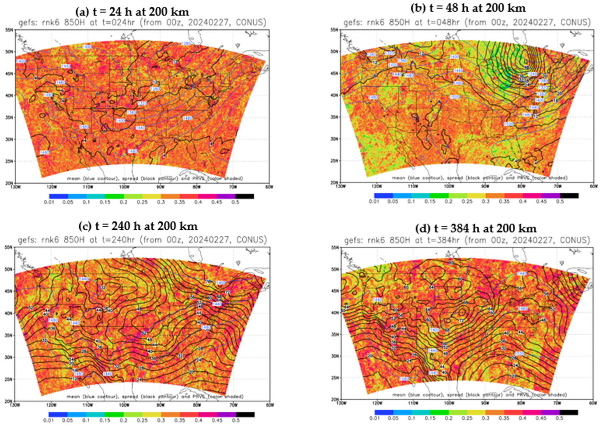
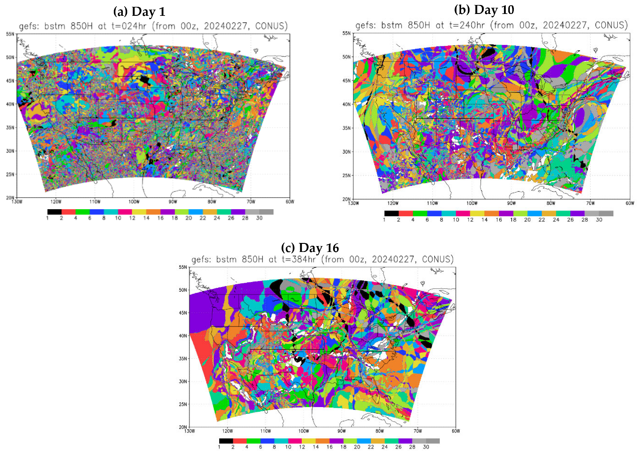
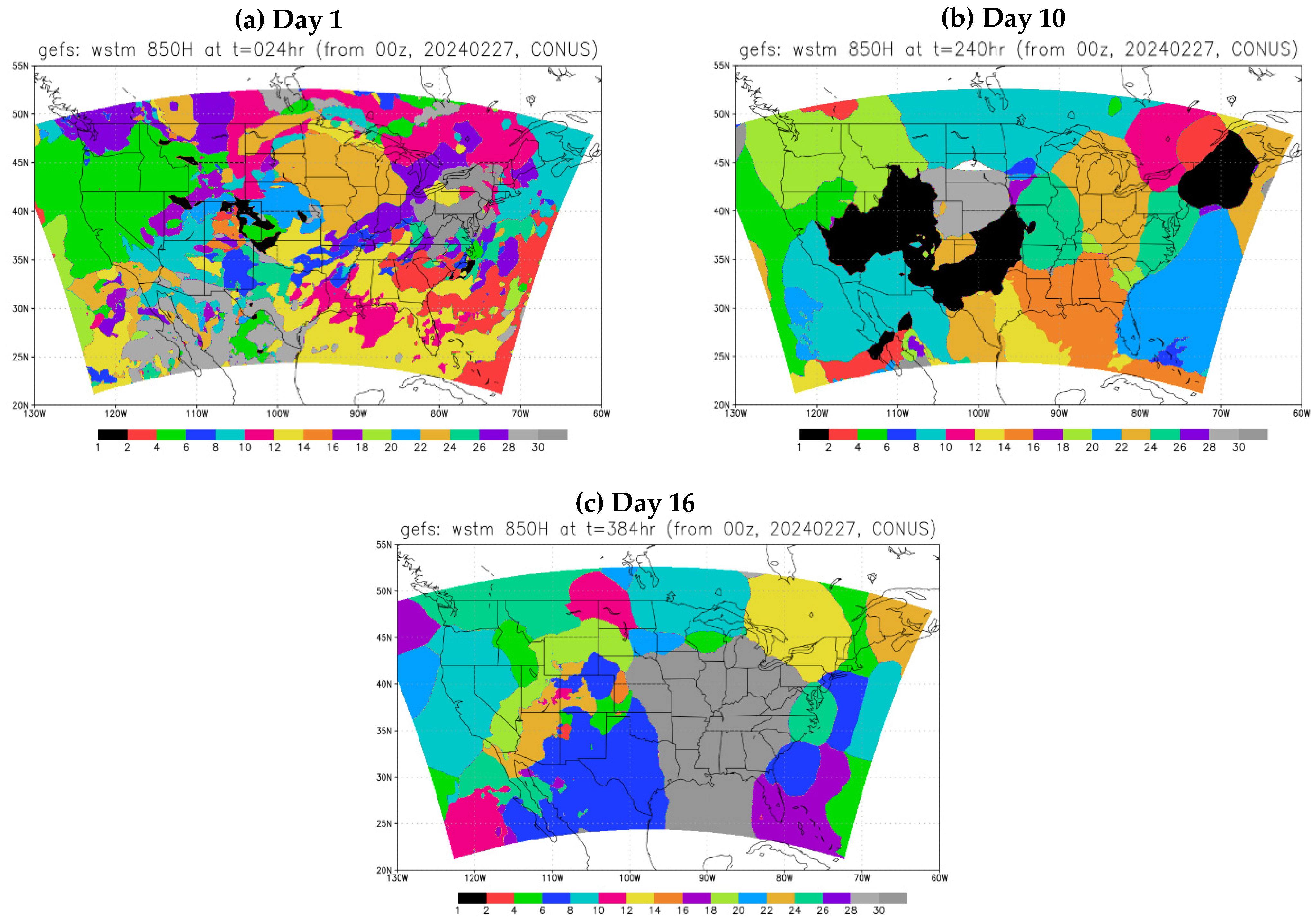
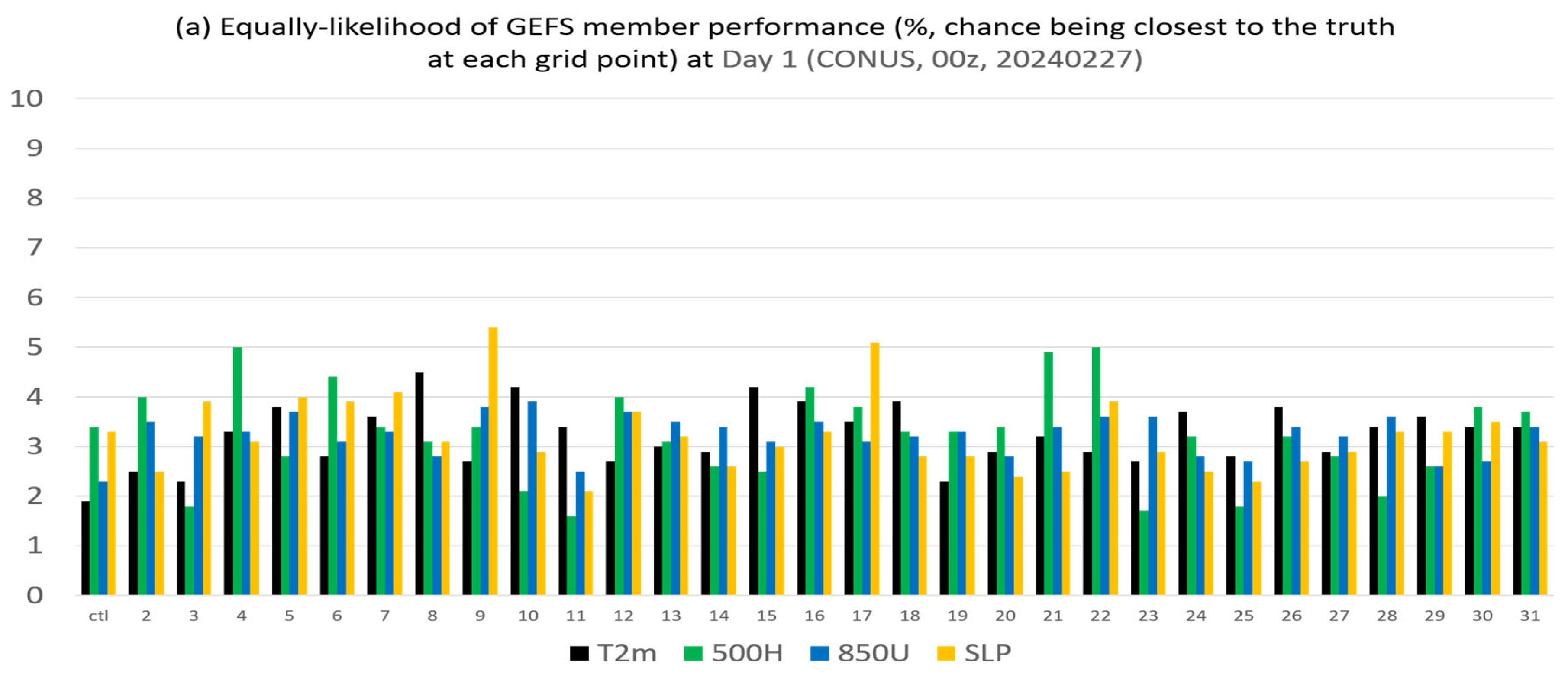
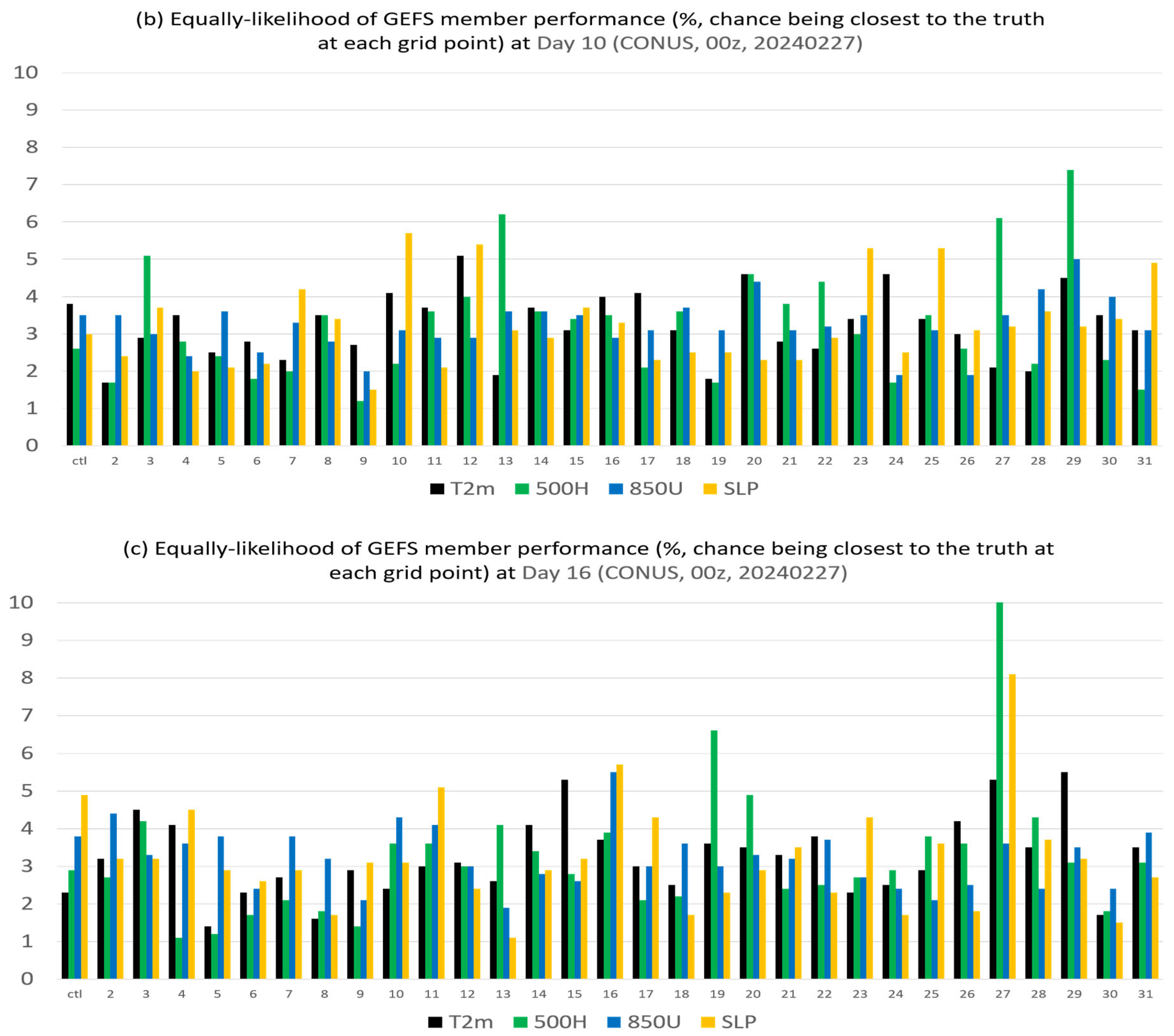
The membership in the best members, worst members, and full members’ performance rank is found to vary significantly (if not randomly) in both space and time. Thus, it will be challenging to steadily extract “correct” information out of an ensemble cloud in advance. This reminds us of the chaotic nature of the atmosphere and emphasizes that the primary mission of an ensemble forecast should provide a spectrum of probable outcomes of a future weather event but not a single outcome.
(2)
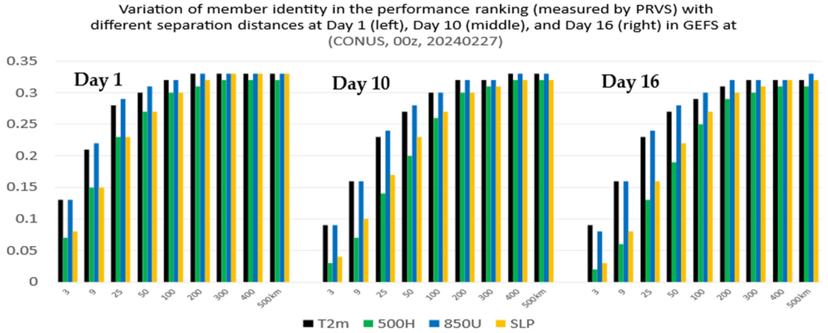
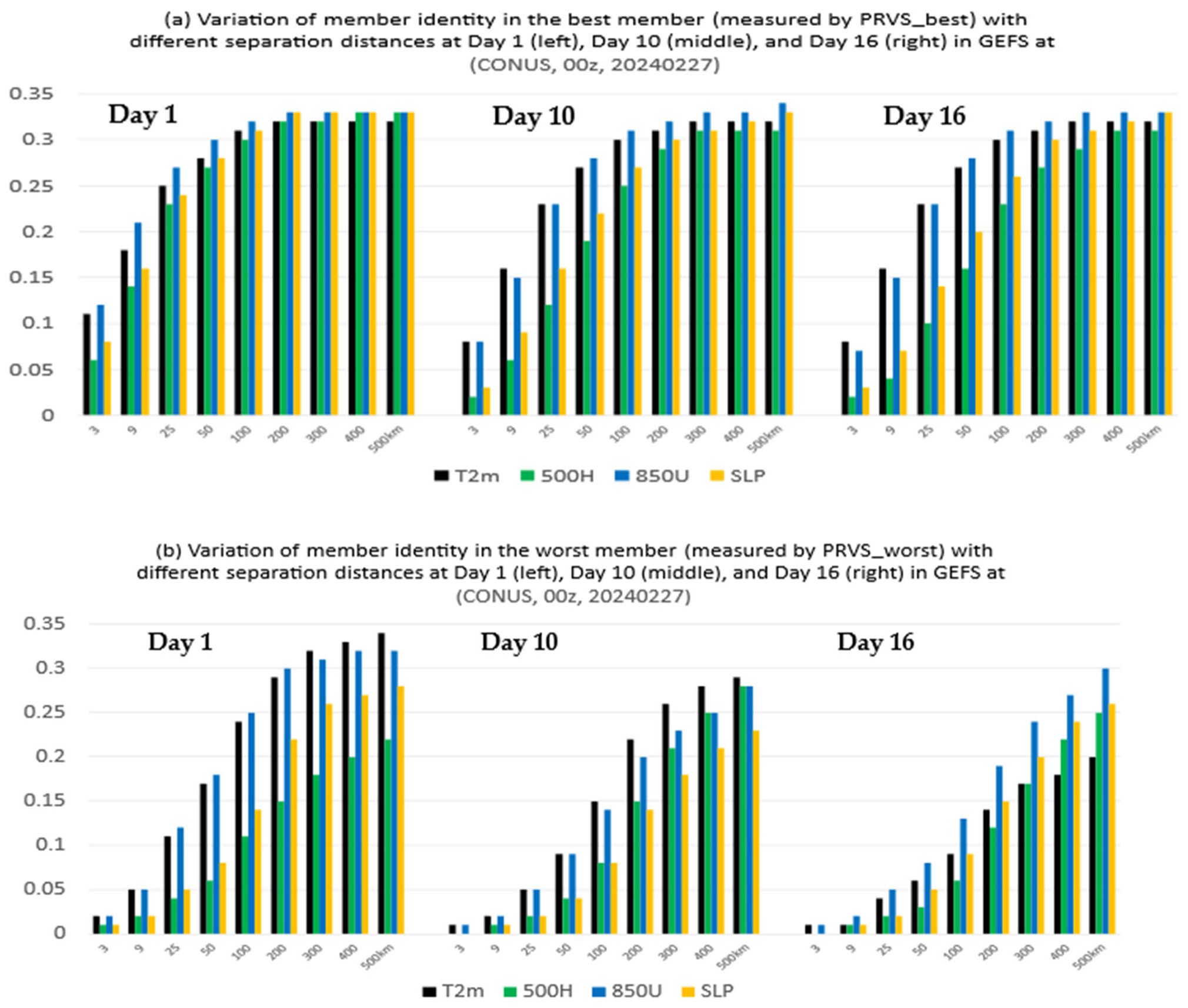
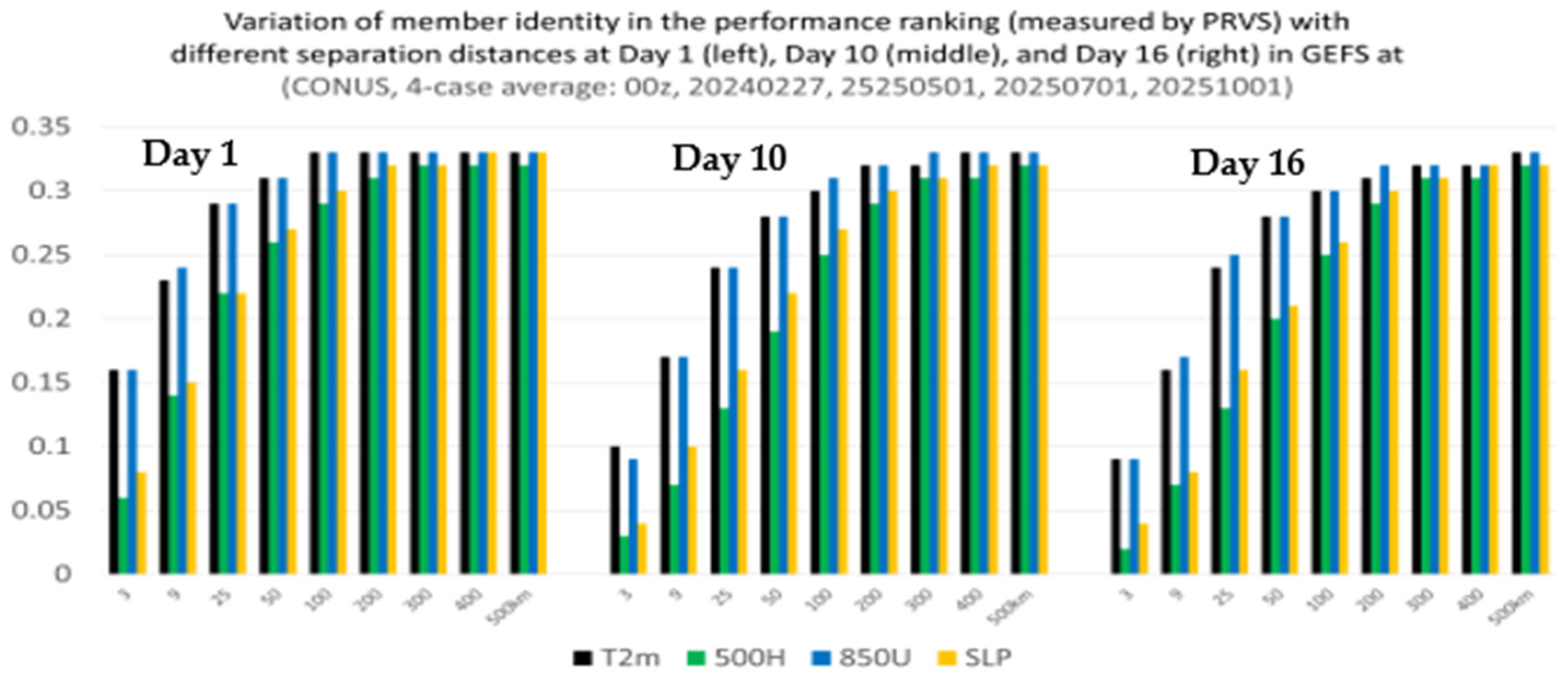
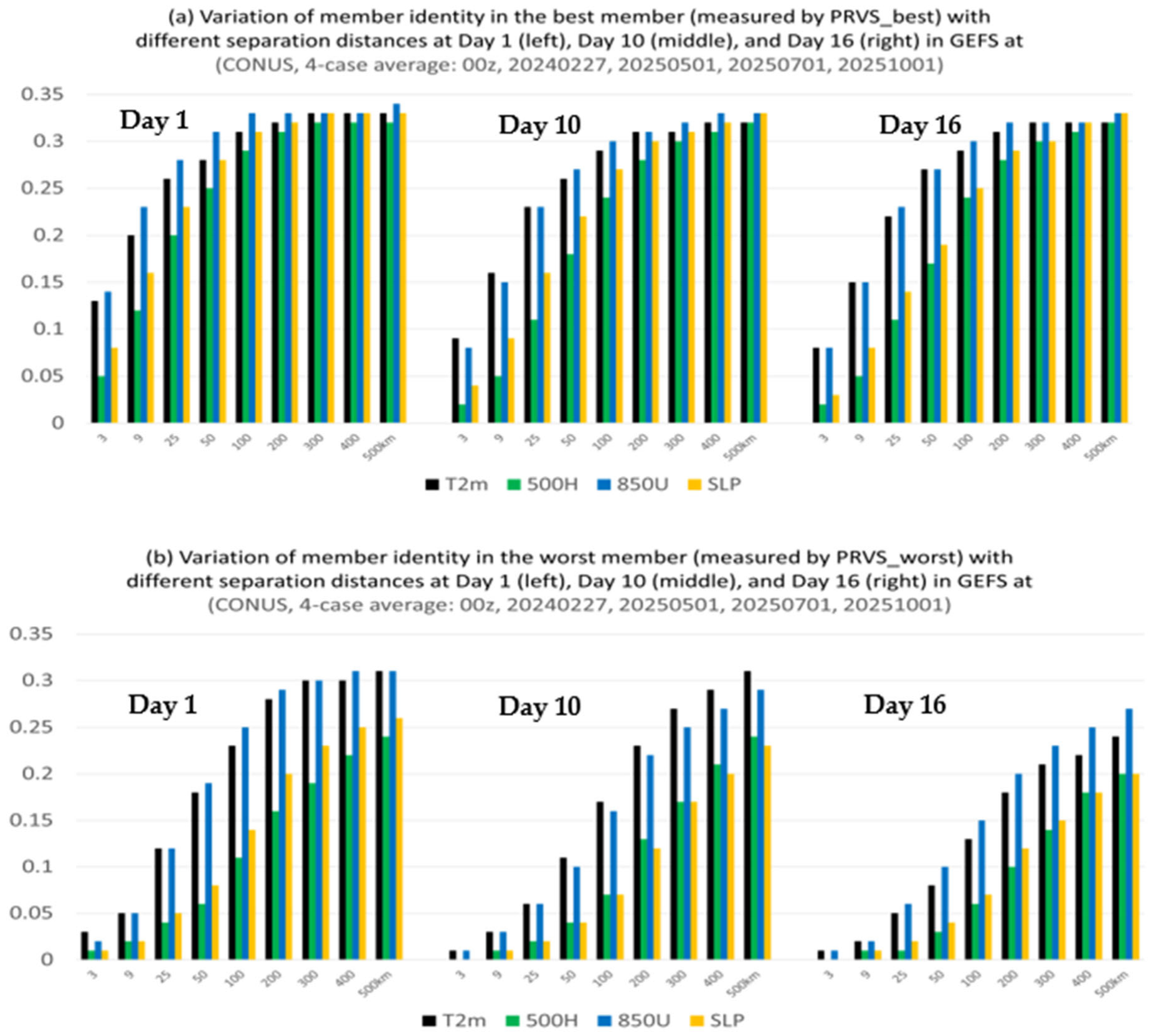
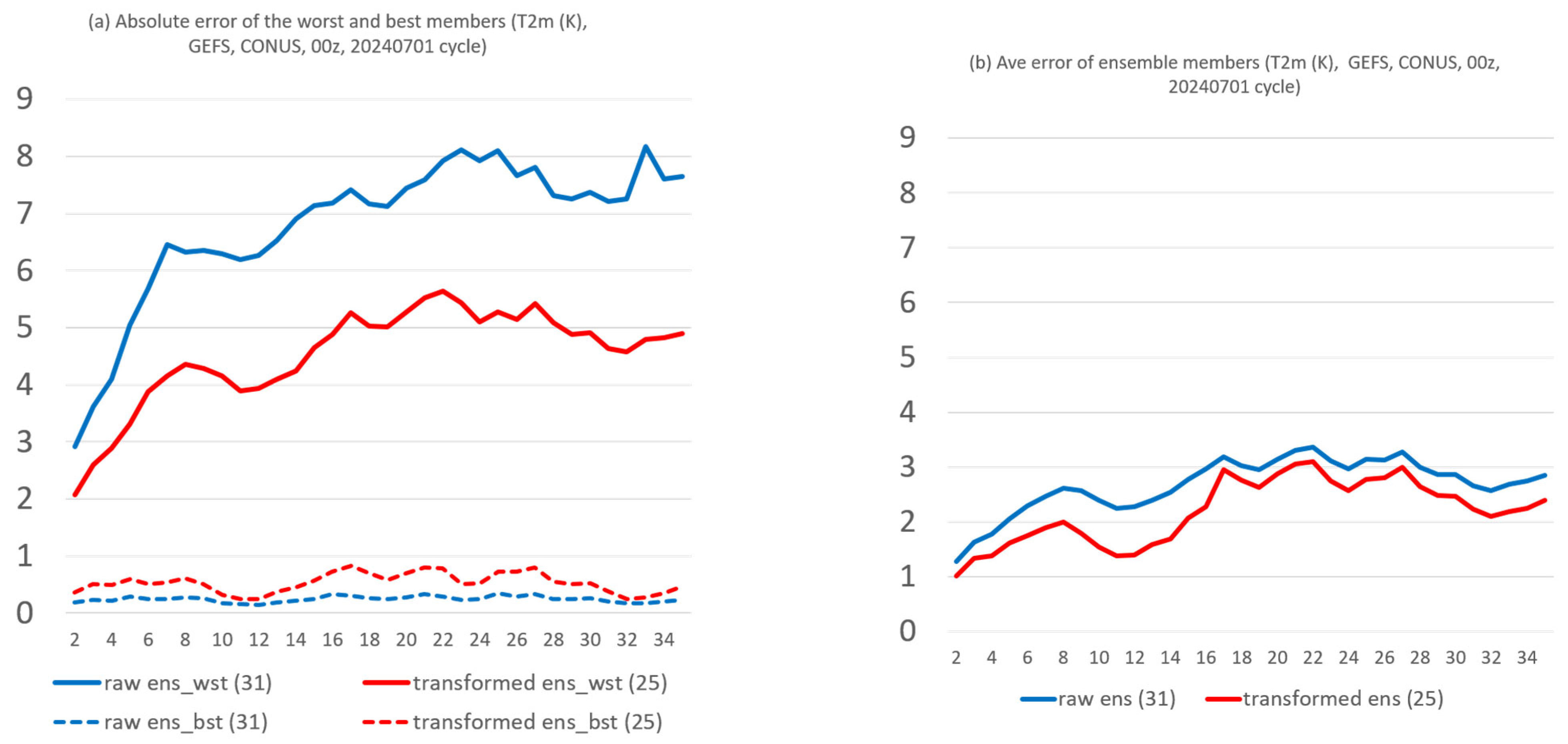
From a forecast calibration point of view, there are a few encouraging results that could be explored as possible ensemble post-processing methods. First, the member identity in the best forecast varies much more rapidly than that of the worst forecast across the space, which hints that the bad forecasts could be relatively easier to identify and separate. Therefore, ensemble post-processing should focus on bad performers rather than good performers by excluding a few worst outliers to produce a more accurate and reliable final forecast product, especially for an over-dispersive ensemble. This exclusion of bad performers should work more effectively for longer time range forecasts given the fact that the membership variation decreases with forecast length for both the best and worst members. Following this finding, a new ensemble post-processing method called “transformed ensemble” is demonstrated as a proof of concept. In-depth research into the transformed ensemble method is ongoing and will be reported separately in due course.
(3)
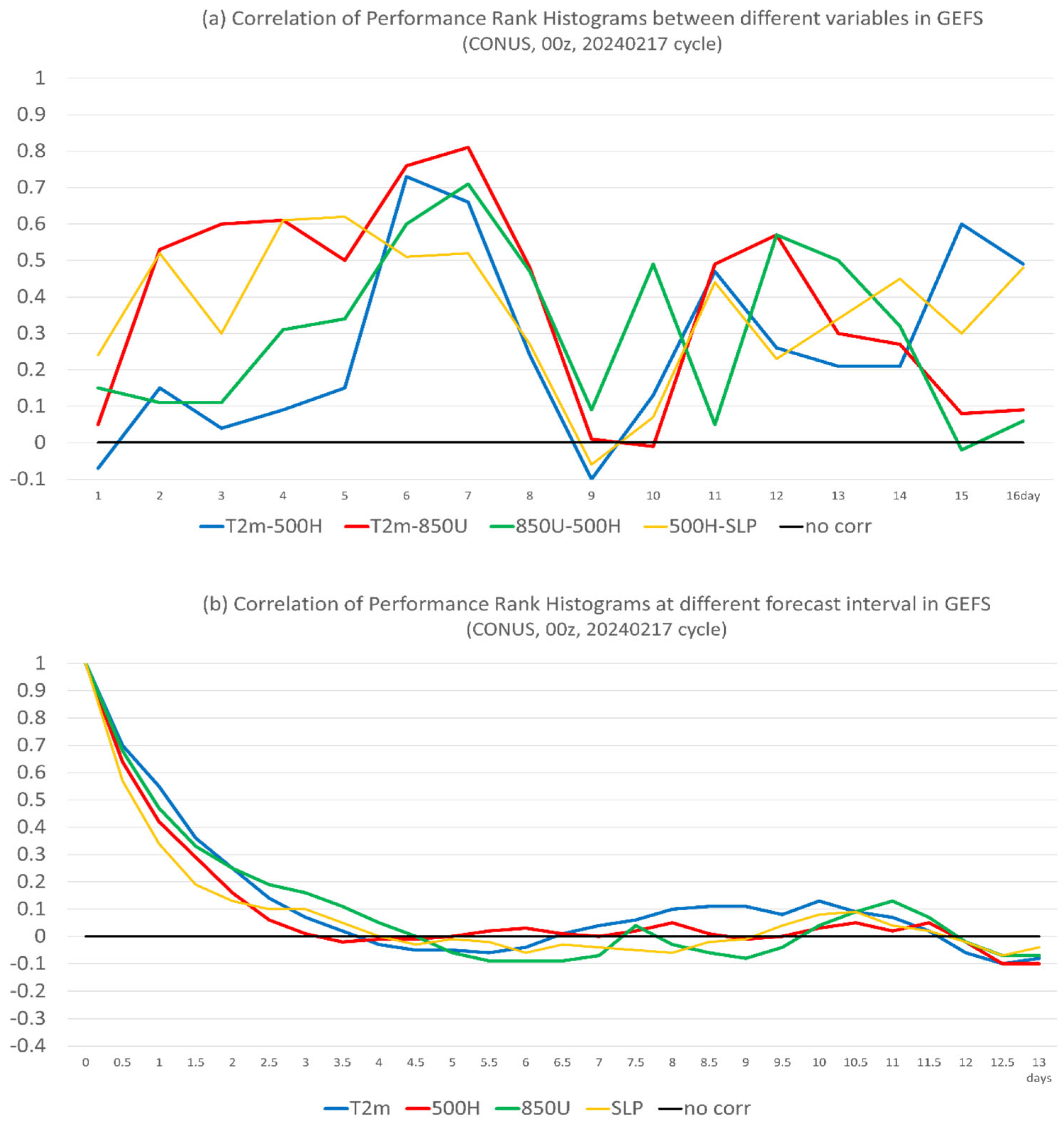
Second, the performance rank histograms are positively correlated between different forecast times if the difference is less than about 2–3 days, and there is no correlation if the forecast time has a difference of more than three days. The shorter time memory of the ensemble member’s relative performance implies that the potential value of using the performance of an earlier-hour forecast to calibrate a later-hour forecast will be limited in ensemble post-processing. For example, based on this result, we can anticipate that the sensitivity-based ensemble subletting approach will not work well beyond 2–3 days in real-world practice. However, it is still possible to calibrate short-range weather forecasts about 1–2 days in advance.
(4)
Third, the fact that members’ performance rank has similarities to each other (positively correlated) among different variables implies that it is possible to use some variables as predictors to calibrate other variables for both short- and long-range forecasts.
The results (2)–(4) could serve as guidance for the future development of ensemble post-processing methods. AI/ML (e.g., Lam et al., 2023 [22]; Bi et al., 2023 [23]) could also lead to significant progress in these developments. Since the current version of the PRVS considers only the order of members but not the magnitude of members’ differences, it could be improved further. Ensemble spread measures the “width” or magnitude of uncertainty, while the PRVS measures the “motion” of uncertainty (how active ensemble members are flipping around in terms of performance). It will be interesting to investigate the relationship between the PRVS and spread. It is observed that some kind of relationship did exist between membership variation and flow regime (cf. Figure 8 and Figure 9), which is another interesting topic to investigate in the future. In this study, the PRVS was applied only to basic atmospheric variables (T, H, U, SLP…); however, it could also be applied to actual weather phenomena such as heavy rain, cyclones, fog, low-visibility conditions, etc.

Funding

This research received no external funding.

Institutional Review Board Statement

Not applicable.

Informed Consent Statement

Not applicable.

Data Availability Statement

The data can be downloaded from NCEP’s operational products inventory under GFS Ensemble Forecast System (GEFS) at https://www.nco.ncep.noaa.gov/pmb/products/gens/ (accessed on 7 July 2025).

Acknowledgments

Jie Feng and another anonymous reviewer are appreciated for their insightful reviews, which helped us to improve the quality of the revised manuscript.

Conflicts of Interest

The author declares no conflict of interest.

References

  1. Lorenz, E.N. Deterministic nonperiodic flow. J. Atmos. Sci. 1963, 20, 130–141. [Google Scholar] [CrossRef]
  2. Lorenz, E.N. A study of the predictability of a 28-variable atmospheric model. Tellus 1965, 17, 321–333. [Google Scholar] [CrossRef]
  3. Lorenz, E.N. The Essence of Chaos; University of Washington Press: Seattle, WA, USA, 1993; 240p. [Google Scholar]
  4. Thompson, P.D. Uncertainty of initial state as a factor in the predictability of large scale atmospheric flow patterns. Tellus 1957, 9, 275–295. [Google Scholar] [CrossRef]
  5. Du, J.; Berner, J.; Buizza, R.; Charron, M.; Houtekamer, P.; Hou, D.; Jankov, I.; Mu, M.; Wang, X.; Wei, M.; et al. Ensemble methods for meteorological predictions. In Handbook of Hydrometeorological Ensemble Forecasting; Duan, Q., Pappenberger, F., Wood, A., Cloke, H.L., Schaake, J., Eds.; Springer: Berlin/Heidelberg, Germany, 2018; p. 52. [Google Scholar] [CrossRef]
  6. Buizza, R.; Du, J.; Toth, Z.; Hou, D. Major operational ensemble prediction systems (EPS) and the future of EPS. In Handbook of Hydrometeorological Ensemble Forecasting; Duan, Q., Pappenberger, F., Wood, A., Cloke, H.L., Schaake, J., Eds.; Springer: Berlin/Heidelberg, Germany, 2018; p. 43. [Google Scholar] [CrossRef]
  7. Toth, Z.; Kalnay, E. Ensemble forecasting at NCEP: The generation of perturbations. Bull. Amer. Meteor. Soc. 1993, 74, 2317–2330. [Google Scholar] [CrossRef]
  8. Molteni, F.; Buizza, R.; Palmer, T.N.; Petroliagis, T. The ECMWF Ensemble Prediction System: Methodology and validation. Q. J. Roy. Meteor. Soc. 1996, 122, 73–119. [Google Scholar] [CrossRef]
  9. Houtekamer, P.L.; Lefaivre, L.; Derome, J.; Ritchie, H.; Mitchell, H.L. A system simulation approach to ensemble prediction. Mon. Weather Rev. 1996, 124, 1225–1242. [Google Scholar] [CrossRef]
  10. Du, J.; Mullen, S.L.; Sanders, F. Short-range ensemble forecasting of quantitative precipitation. Mon. Weather Rev. 1997, 125, 2427–2459. [Google Scholar] [CrossRef]
  11. Chen, J.; Zhu, Y.; Duan, W.; Zhi, X.; Min, J.; Li, X.; Deng, G.; Yuan, H.; Feng, J.; Du, J.; et al. A review on development, challenges, and future perspectives of ensemble forecast. J. Meteorol. Res. 2025, 39, 534–558. [Google Scholar] [CrossRef]
  12. Zhou, X.; Zhu, Y.; Hou, D.; Fu, B.; Li, W.; Guan, H.; Sinsky, E.; Kolczynski, W.; Xue, X.; Luo, Y.; et al. The Development of the NCEP Global Ensemble Forecast System Version 12. Weather Forecast. 2022, 37, 1069–1084. [Google Scholar] [CrossRef]
  13. Fu, B.; Zhu, Y.; Guan, H.; Sinsky, E.; Yang, B.; Xue, X.; Pegion, P.; Yang, F. Weather to seasonal prediction from the UFS Coupled Global Ensemble Forecast System. Weather Forecast. 2024; in press. [Google Scholar] [CrossRef]
  14. Lin, S.J.; Putman, W.; Harris, L. FV3: The GFDL Finite-Volume Cubed-Sphere Dynamical Core (Version 1), NWS/NCEP/EMC. 2017. Available online: https://www.gfdl.noaa.gov/wp-content/uploads/2020/02/FV3-Technical-Description.pdf (accessed on 23 July 2025).
  15. Houtekamer, P.L.; Mitchell, H.L. Data assimilation using an ensemble Kalman filter technique. Mon. Weather Rev. 1998, 126, 196–811. [Google Scholar] [CrossRef]
  16. Kleist, D.T.; Ide, K. An OSSE-based evaluation of hybrid variational-ensemble data assimilation for the NCEP GFS, Part I: System description and 3D-hybrid results. Mon. Weather Rev. 2015, 143, 433–451. [Google Scholar] [CrossRef]
  17. Du, J.; Zhou, B. A dynamical performance-ranking method for predicting individual ensemble member’s performance and its application to ensemble averaging. Mon. Weather Rev. 2011, 129, 3284–3303. [Google Scholar] [CrossRef]
  18. Bright, D.R.; Nutter, P.A. On the challenges of identifying the “best” ensemble member in operational forecasting. In Proceedings of the 16th Conference on Numerical Weather Prediction/20th Conference on Weather Analysis and Forecasting, Seattle, WA, USA, 14 January 2004; Available online: https://ams.confex.com/ams/84Annual/techprogram/paper_69092.htm (accessed on 23 July 2025).
  19. Du, J. An assessment of ensemble forecast performance: Where we are and where we should go. In Proceedings of the 33rd Conference on Weather Analysis and Forecasting (WAF)/29th Conference on Numerical Weather Prediction (NWP), New Orleans, LA, USA, 12–16 January 2025. [Google Scholar]
  20. Du, J.; Tabas, S.S.; Wang, J.; Levit, J. Understanding similarities and differences between data-driven based and physics model-based ensemble forecasts. NCEP Off. Notes 2025, 523, 31p. [Google Scholar] [CrossRef]
  21. Ancell, B.C. Improving High-Impact Forecasts Through Sensitivity-Based Ensemble Subsets: Demonstration and Initial Tests. Weather Forecast. 2016, 31, 1019–1036. [Google Scholar] [CrossRef]
  22. Lam, R.; Sanchez-Gonzalez, A.; Willson, M.; Wirnsberger, P.; Fortunato, M.; Alet, F.; Ravuri, S.; Ewalds, T.; Eaton-Rosen, Z.; Hu, W.; et al. Graphcast: Learning skillful medium-range global weather forecasting. Science 2023, 382, 1416–1421. [Google Scholar] [CrossRef] [PubMed]
  23. Bi, K.; Xie, L.; Zhang, H.; Chen, X.; Gu, X.; Tian, Q. Accurate medium range global weather forecasting with 3-D neural networks. Nature 2023, 619, 533–538. [Google Scholar] [CrossRef] [PubMed]
Figure 1. Definition, calculation, and examples of the “Performance Rank Variation Score (PRVS)” for an ensemble with N members between Point A and Point B. It is a positively oriented measure, i.e., the larger the PRVS value is, the larger the membership position variation in the member’s performance rank over spatial or temporal space. The PRVS value ranges from 0 to 0.5.
Meteorology 04 00020 g001
Figure 2. The Performance Rank Variation Score (PRVS) for the 31-member GEFS’s 48 h forecast of 850H, calculated between two neighboring grid points in different separation distances: (a) 3 km; (b) 9 km; (c) 25 km; (d) 50 km; (e) 100 km; (f) 200 km; (g) 300 km; and (h) 400 km. Color shading is the PRVS, the black contour is the ensemble spread of 850H, and the blue contour is the ensemble mean of 850H. The GEFS forecast is initiated from 00z, 27 February 2024, and projected for 16 days (384 h).
Meteorology 04 00020 g002aMeteorology 04 00020 g002b
Figure 3. The Performance Rank Variation Score (PRVS) for the GEFS forecasts of 850H, calculated between two neighboring grid points with separation distance D = 25 km at four different forecast lengths from short range to long range: (a) day 1 (short range); (b) day 2 (short range); (c) day 10 (medium range); and (d) day 16 (long range). Color shading is the PRVS, the black contour is the ensemble spread of 850H, and the blue contour is the ensemble mean of 850H.
Meteorology 04 00020 g003
Figure 4. Same as Figure 3 but for the separation distance of 200 km.
Meteorology 04 00020 g004
Figure 5. Variation in the Performance Rank Variation Score (PRVS) with the separation distances of the four variables (T2m, 500H, 850U, and SLP) for the full member’s performance ranking at days 1 (left panel), 10 (middle), and 16 (right). The PRVS values are averaged over the entire verification domain CONUS. The GEFS forecast is initiated from 00z, 27 February 2024, and projected for 16 days (384 h).
Meteorology 04 00020 g005
Figure 6. Same as Figure 5 but for (a) the best member and (b) the worst member.
Meteorology 04 00020 g006
Figure 7. Spatial distribution of the member identity in the best member from the GEFS forecast of 850H. Three forecast ranges are shown: (a) short range (day 1), (b) medium range (day 10), and (c) long range (day 16). Different colors represent different ensemble members. The GEFS forecast is initiated from 00z, 27 February 2024, and projected for 16 days (384 h).
Meteorology 04 00020 g007
Figure 8. Same as Figure 7 but for the worst member.
Meteorology 04 00020 g008
Figure 9. The GFS analysis of 850H fields for the winter case (20240227) corresponding to (a) day 1, (b) day 10, and (c) day 16 of the other figures such as Figure 3, Figure 4, Figure 5, Figure 6, Figure 7 and Figure 8.
Meteorology 04 00020 g009
Figure 10. Same as Figure 5 but for the average result of the four cases (winter, spring, summer, and fall).
Meteorology 04 00020 g010
Figure 11. Same as Figure 6 but for the average result of the four cases (winter, spring, summer, and fall).
Meteorology 04 00020 g011
Figure 12. (a) Absolute forecast errors of the worst (solid curves) and best member (dashed curves) for T2m from the transformed ensemble (in red) and the raw ensemble (in blue), respectively. (b) The average absolute error of ensemble members. The GEFS forecast is initiated from 00z, 1 July 2024, and projected for 35 days (840 h).
Meteorology 04 00020 g012
Figure 13. Performance rank histogram of the four selected variables (T2m, 500H, 850U, and SLP) for (a) short-range (day 1), (b) medium-range (day 10), and (c) long-range (day 16) forecasts over the 31 GEFS members. The values are averaged over the entire verification domain CONUS. The GEFS forecast is initiated from 00z, 27 February 2024, and projected for 16 days (384 h).
Meteorology 04 00020 g013aMeteorology 04 00020 g013b
Figure 14. Correlation of performance rank histograms (Figure 13) between (a) different variables (“cross-variable correlation”) and (b) different forecast times (with 12 h increments: t + 00, t + 12, t + 24, t + 36, t + 48, … hours and averaged over the entire forecast length from 12 h to 384 h) (“cross-time correlation”) for the four selected variables (T2m, 500H, 850U, and SLP) of the GEFS forecasts. The GEFS forecast is initiated from 00z, 27 February 2024, and projected for 16 days (384 h).
Meteorology 04 00020 g014
Disclaimer/Publisher’s Note: The statements, opinions and data contained in all publications are solely those of the individual author(s) and contributor(s) and not of MDPI and/or the editor(s). MDPI and/or the editor(s) disclaim responsibility for any injury to people or property resulting from any ideas, methods, instructions or products referred to in the content.

