Trends of Liquid Water Path of Non-Raining Clouds as Derived from Long-Term Ground-Based Microwave Measurements near the Gulf of Finland

Abstract

Quantifying long-term variations in the cloud liquid water path (LWP) is crucial to obtain a better understanding of the processes relevant to cloud–climate feedback. The 12-year (2013–2024) time series of LWP values obtained from ground-based measurements by the RPG-HATPRO radiometer near the Gulf of Finland is analysed, and the linear trends of the LWP for different sampling subsets of data are assessed. These subsets include all-hour, daytime, and night-time measurements. Two different approaches have been used for trend assessment, which produced similar results. Statistically significant linear trends have been detected for most data subsets. The most pronounced general trend over the period 2013–2024 has been detected for the daytime LWP, and it constitutes −0.0011 ± 0.00015 kg m⁻² yr⁻¹. This trend is driven mainly by the daytime LWP trend for the warm season (May–July, −0.0014 ± 0.00015 kg m⁻² yr⁻¹), which is considerably larger than the trend for the cold season (November–January, −0.00064 ± 0.00026 kg m⁻² yr⁻¹). Additionally, the analysis shows that the absolute number of clear-sky measurements decreased approximately by a factor of 4 if the years 2013 and 2024 are compared.

1. Introduction

Remote sensing of the atmosphere by ground-based microwave radiometers (MWRs) is widely used to monitor different parameters of the atmospheric state and composition. In particular, measurements of temperature and humidity profiles in the troposphere together with the cloud liquid water path (LWP—the total mass of cloud liquid water droplets in the atmosphere above a unit surface area) have become routine ones. A detailed description of the physical fundamentals of ground-based microwave radiometry, as well as measurement techniques, retrieval strategies, and concepts of modern microwave instruments, can be found in the review by Westwater et al. [1]. Ground-based MWRs operate under nearly all weather conditions, continuously, automatically, and with high temporal resolution. These advantages have stimulated the commercial production of microwave radiometers for atmospheric sounding and their continuous improvement. In this respect, one can mention, in particular, radiometers of the RPG-HATPRO type (Radiometer Physics GmbH—Humidity and Temperature Profiler) of different generations, which have been previously used in a large number of atmospheric studies [2,3,4,5,6,7,8,9,10,11]. For the sake of exchanging information in the MWR user community, the International Network of Ground-based Microwave Radiometers has been established (MWRnet, http://cetemps.aquila.infn.it/mwrnet/, accessed on 26 March 2025).

Among the most recent studies, there are ones aimed at practical applications of the MWR remote sensing products: temperature and humidity profiles, LWP, and integrated water vapour. It is worth mentioning the works by Martinet et al. [12] and by Thomas et al. [13] in which a unique network of eight ground-based HATPRO microwave radiometers has been deployed over the southwestern part of France in order to improve fog forecasting. The study by Cimini et al. [14] has addressed the specific question of the quality of atmospheric stability retrievals from MWR measurements for wind energy applications in different climates. In this study, the ability of commercially available MWRs to retrieve atmospheric temperature within the first 2 km and to provide potential temperature gradients in the vertical range of wind turbine rotors has been assessed against in situ radiosonde measurements. Karavaev et al. [15] estimated the capabilities of microwave radiometry in improving the diagnosis of the synoptic and mesoscale structure of atmospheric fronts and in improving methods for forecasting severe weather events associated with the development of convective clouds, thunderstorms, and precipitation.

Currently, establishing an operational network of MWRs is a goal that is supported by several initiatives and international organisations. The EU COST Action CA 40 18,235 PROBE (PROfiling the atmospheric Boundary layer at European scale, https://www.cost.eu/actions/CA18235/, accessed on 26 March 2025) and the European Research Infrastructure for the observation of Aerosol, Clouds, and Trace gases (ACTRIS, https://www.actris.eu/, accessed on 26 March 2025) focus on establishing continent-wide quality and observation standards for MWR networks. The German Weather Service also investigates the potential of MWR networks for improving short-term weather forecasts over Germany [16].

As mentioned above, the cloud LWP is one of atmospheric parameters that are retrieved from ground-based microwave observations. It should be emphasised that the retrieval accuracy of this quantity is high and is sufficient for using LWP data from ground-based microwave measurements as reference data in validation campaigns for space-borne LWP retrievals. It should also be noted that the LWP is one of the most essential cloud parameters. It is well-known that the role of clouds in the climate system is very important since clouds are linked to the global hydrologic cycle and to the global radiation budget. Therefore, the LWP data from ground-based MWRs, which have been operating for long periods of time, can make a considerable contribution to regional climatological studies. So far, the LWP climatology and trends have been investigated intensively using data from different space-borne instruments [17]. The methodologies of LWP retrievals by these instruments and the characteristics of corresponding datasets vary greatly: some are based on measurements of self-emitted microwave radiation; others are based on measurements of reflected solar radiation in visible (VIS) and near-infrared (NIR) ranges. Microwave measurements of the LWP from space provide information over oceans only. VIS and NIR measurements of reflected solar radiation provide information over land and oceans but only under solar illumination conditions. A detailed discussion of the advantages and weaknesses of the methods of LWP retrievals from space can be found in the paper by Manaster et al. [18].

So far, the studies devoted to the analysis of the long-term trends of the cloud LWP obtained from ground-based microwave observations are not numerous. In the present paper, we make an attempt to derive the magnitude of the LWP trends from the LWP time series obtained from multi-year ground-based microwave measurements by the HATPRO radiometer located in Northern Europe near the coastline of the Gulf of Finland.

2. Experimental Setup and Retrieval Method for LWP

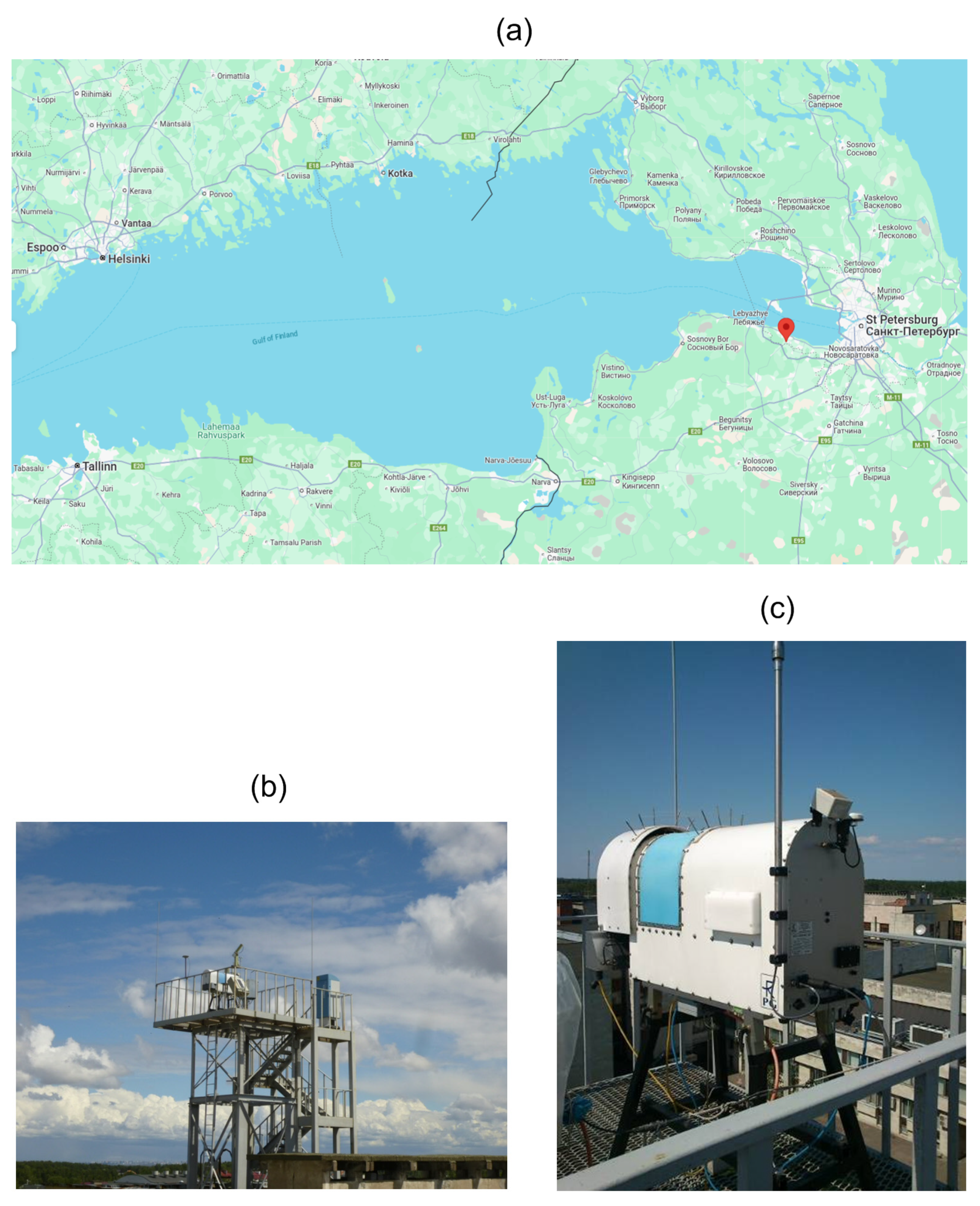
The 14-channel microwave radiometer HATPRO, generation G3 (Figure 1c) is installed on the metal platform on the roof of the building of the Research Institute of Physics, St. Petersburg State University (Figure 1b). The geographical coordinates of the instrument location are 59.88107° N, 29.82597° E (Figure 1a). The altitude of the instrument above sea level is 56 m. Two types of viewing geometry are used: zenith direction and angular scanning. For angular scanning, the instrument is facing north. The integration time for a single measurement is 1 s, and the sampling interval between single measurements is 1–2 s. The instrument performs continuous observations in unattended mode. Periods of rain events are excluded from analysis since the data during these periods are erroneous due to two reasons: first, the radome of the instrument is wet, and second, the microwave radiative transfer model, which is used, does not account for scattering on large rain drops. The device is regularly calibrated using liquid nitrogen. The experimental setup and the measurement routine are described in detail in the papers by Kostsov et al. [19,20].

The raw data are the brightness temperature values registered in 14 spectral channels. Seven channels located in the water vapour line with the central wavelength of 1.35 cm and in the window of transparency near 0.8 cm are sensitive to the atmospheric humidity profile and to the cloud liquid water path. Seven channels in the 0.5 cm oxygen absorption band are sensitive to the temperature profile. The manufacturer of the radiometer has provided the built-in retrieval algorithm based on the linear regression technique; however, we used the original so-called “physical” retrieval algorithm. In this physical algorithm, the inverse problem has been formulated on the basis of the linearised radiative transfer equation:

$$y-y_0=A(x-x_0)$$

(1)

where the components of vector y are the values of the brightness temperature in 14 spectral channels, A is the matrix of the “forward” operator, and vector x is the combined vector of the vertical profiles of temperature, pressure, absolute humidity, and cloud liquid water density. The subscript “0” denotes reference values used for the calculations of variations of enumerated quantities. Equation (1) is the classical equation of the ill-posed problem of atmospheric remote sensing. It is solved by the iterative optimal estimation algorithm accounting for additional a priori information and constraints. In particular, we used the hydrostatic equilibrium constraint for coupling the temperature and pressure profiles and additional direct in situ measurements of the temperature and relative humidity near the surface provided by built-in sensors in the HATPRO instrument. The details of the multi-parameter retrieval algorithm accounting for different types of a priori information and constraints are described in [21], and its application to the processing of microwave measurements is described in [19,20,22]. In the present study, the target parameter is the LWP; therefore, we do not discuss here the retrievals of the temperature and humidity profiles and the integrated water vapour.

It should be noted that the LWP values have been obtained by integration of the cloud liquid water density profile. Since ground-based microwave measurements are largely insensitive to the spatial distribution of the cloud liquid water density, we do not consider and analyse the cloud liquid water density profiles. The accuracy of the LWP retrievals has been estimated using measurements under clear-sky conditions. Additionally, for each individual retrieval result, the accuracy has been calculated from the error matrix of the optimal estimation method for a specific atmospheric situation during retrieval. In the warm season, the range of error values is 0.002–0.008 kg m⁻², and in the cold season, it is 0.002–0.005 kg m⁻². The corresponding mean error values are 0.004 kg m⁻² and 0.003 kg m⁻². The data quality control procedure included the calculation and analysis of the spectral residual, analysis of the convergence of the iteration process, and several other steps. All data that did not pass one or more control tests were excluded from consideration.

3. Data Series Overview

The total amount of individual results of LWP retrieval is quite large since routine measurements were made every 1–2 s. For analysis, we selected measurements with a sampling interval equal to 20 s. At the first step of data processing, all results with an LWP larger than 0.4 kg m⁻² have been filtered out since the value of 0.4 kg m⁻² has been reported earlier as a threshold LWP between non-rainy and rainy atmospheres [23]. At the second step of data processing, we used measurements under clear-sky conditions to obtain the estimates of the LWP bias (0.008 kg m⁻²) and of the standard deviation of the LWP (0.002 kg m⁻²). This is a well-established procedure that is described, for example, in previous papers [20,24,25]. After that, all data have been divided into two classes—“clouds” and “clear sky”. The following algorithm has been used:

−

If LWP ≤ 0.012 kg m⁻², then the LWP is assigned a zero value (LWP = 0), and the considered measurement is classified as “clear sky”;

−

If LWP > 0.012 kg m⁻², then the bias is removed (LWP = LWP−0.008 kg m⁻²), and the considered measurement is classified as “clouds”.

Here, the value 0.012 kg m⁻² is the LWP bias plus double the standard deviation. As a result of this procedure, we obtained the data without bias and also a clear distinction between measurements under cloudy and clear-sky conditions. After that, we created six subsets of data, which are described in

Table 1. Description of the data subsets (SZA—solar zenith angle).

Data Subset	Elements Included in a Subset and Data Selection Criterion	Description
A0	LWP > 0, unlimited SZA range	All-hour measurements, cloudy cases only, true LWP
AD	LWP > 0, SZA < 90°	Daytime measurements, cloudy cases only, true LWP
AN	LWP > 0, SZA ≥ 90°	Night-time measurements, cloudy cases only, true LWP
B0	LWP ≥ 0, unlimited SZA range	All-hour measurements, mixed cloudy and clear-sky cases, virtual LWP
BD	LWP ≥ 0, SZA < 90°	Daytime measurements, mixed cloudy and clear-sky cases, virtual LWP
BN	LWP ≥ 0, SZA ≥ 90°	Night-time measurements, mixed cloudy and clear-sky cases, virtual LWP

. There were two reasons for classifying the data into these subsets:

(1)

Subsets of type “A” contain measurements under cloudy conditions only, and so they provide the opportunity to investigate the so-called “intrinsic” properties of clouds. Therefore, we use the term “true LWP” for the LWP in these subsets. Subsets of type “B” are used to study the properties of the atmosphere “as a whole”, and they contain mixed clear-sky measurements and measurements under cloudy conditions. Since we assign a zero LWP to clear-sky measurements, we use the term “virtual LWP” for the LWP in “B” subsets.

(2)

Additional sorting of the data depending on the solar zenith angle gives the opportunity to study the diurnal features of the LWP. The symbols “0”, “D”, and “N” in the data subset designations correspond to all-hour, daytime, and night-time measurements.

For statistical analysis, the following quantities have been calculated for each data subset:

$$\mathrm{Diurnal} \mathrm{mean}:\begin{array}{cc}& \end{array}LW{P}_d={\displaystyle \sum _{0-24hr}LW{P}_i}$$

(2)

$$\mathrm{Monthly} \mathrm{mean}:\begin{array}{cc}& \end{array}LW{P}_m={\displaystyle \sum _{1-31Days}LW{P}_i}$$

(3)

$$\mathrm{Seasonal} \mathrm{mean}:\begin{array}{cc}& \end{array}LW{P}_s={\displaystyle \sum _{Months}LW{P}_i}$$

(4)

where LWP_i denotes an individual measurement, and “Months” denote selected months for specific season. The annual mean values have been calculated using the diurnal mean values rather than individual measurements:

$$\mathrm{Annual} \mathrm{mean}:\begin{array}{cc}& \end{array}LW{P}_y={\displaystyle \sum _{1-366days}LW{P}_d}$$

(5)

This is deliberately carried out in order not to produce misleading results because of the variable duration of the sun illumination period. The observational site is located at a relatively high latitude. As a result, the daytime measurements are prevailing in the summer due to the long sun illumination period, and the night-time measurements are prevailing in the winter. Obviously, seasonal and diurnal variations of the LWP can interfere with each other. If the daytime and night-time measurements have equal weights when the data are averaged, then misleading results can be obtained. Formula (5) helps to avoid such a situation.

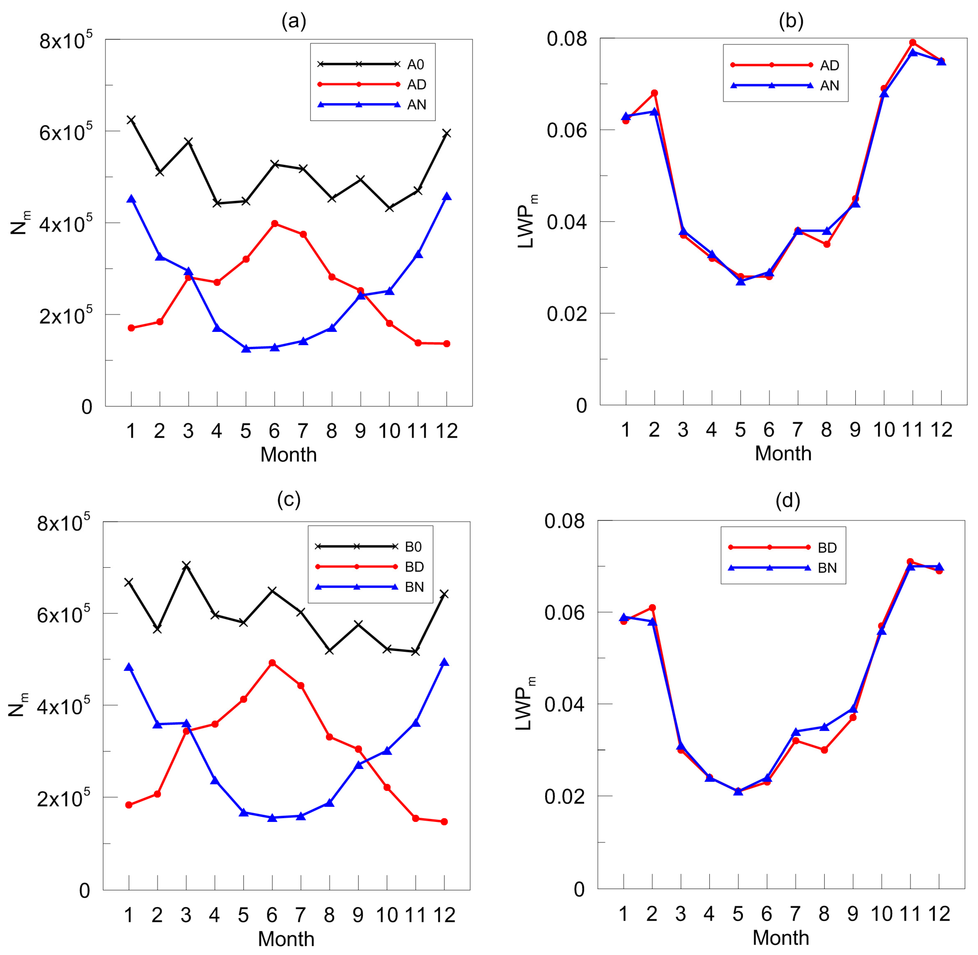
Figure 2a,c demonstrates the seasonal behaviour of the average number of measurements per month N_m in different data subsets. One can see the evident seasonal variability of N_m for the daytime and for the night-time measurements for subsets of the “A” type and of the “B” type. The total number of measurements per month does not vary considerably within a year. Figure 2b,d shows the average seasonal behaviour of the monthly mean LWP values calculated for daytime and night-time subsets. First, we note that the monthly mean daytime and night-time LWP values averaged over the whole period of 2013–2024 are very similar for all months except August. Second, we observe a pronounced seasonal variation of the monthly mean LWP values, with minimal values in May and June and maximal values in January, February, October, November, and December.

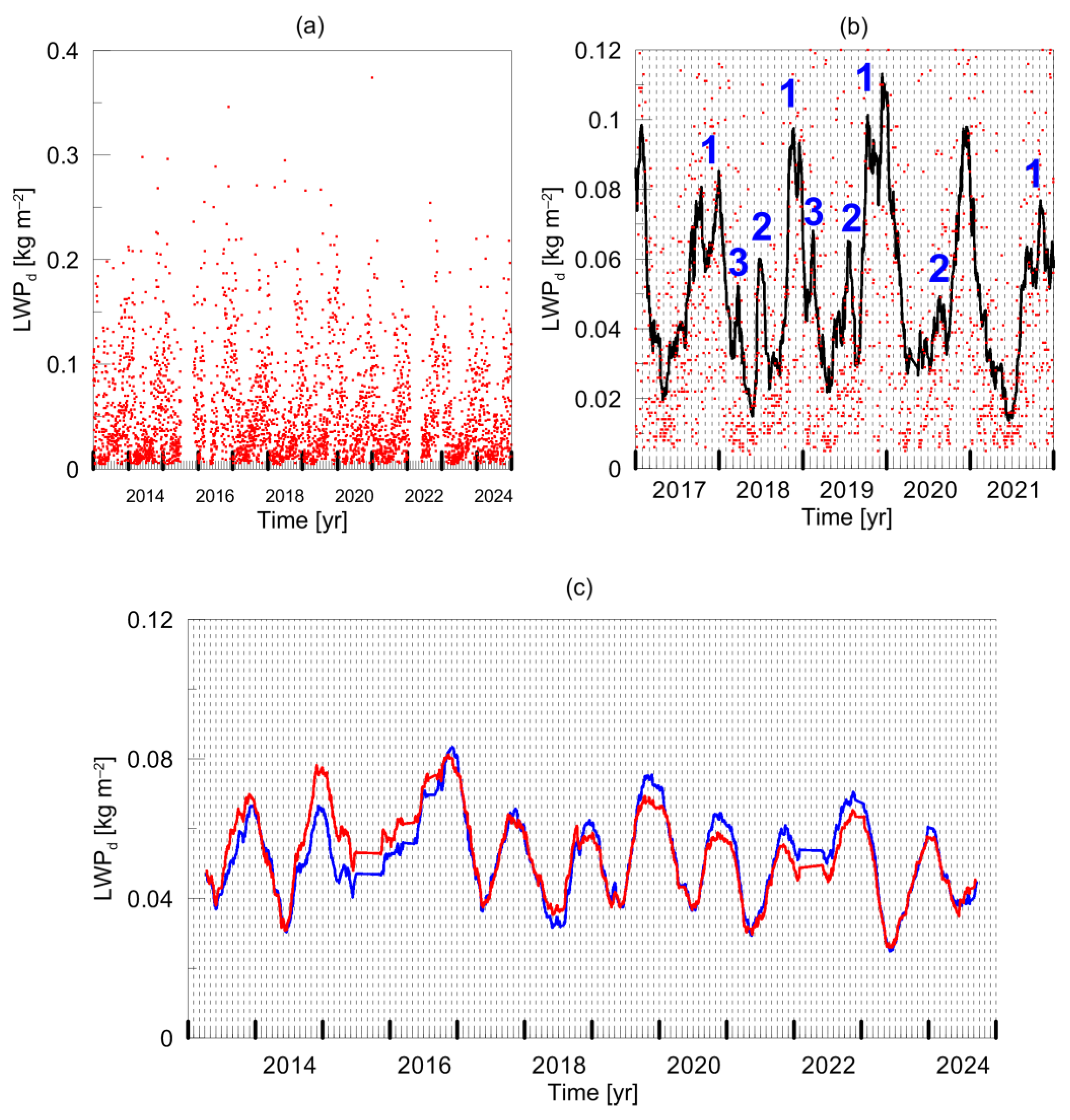
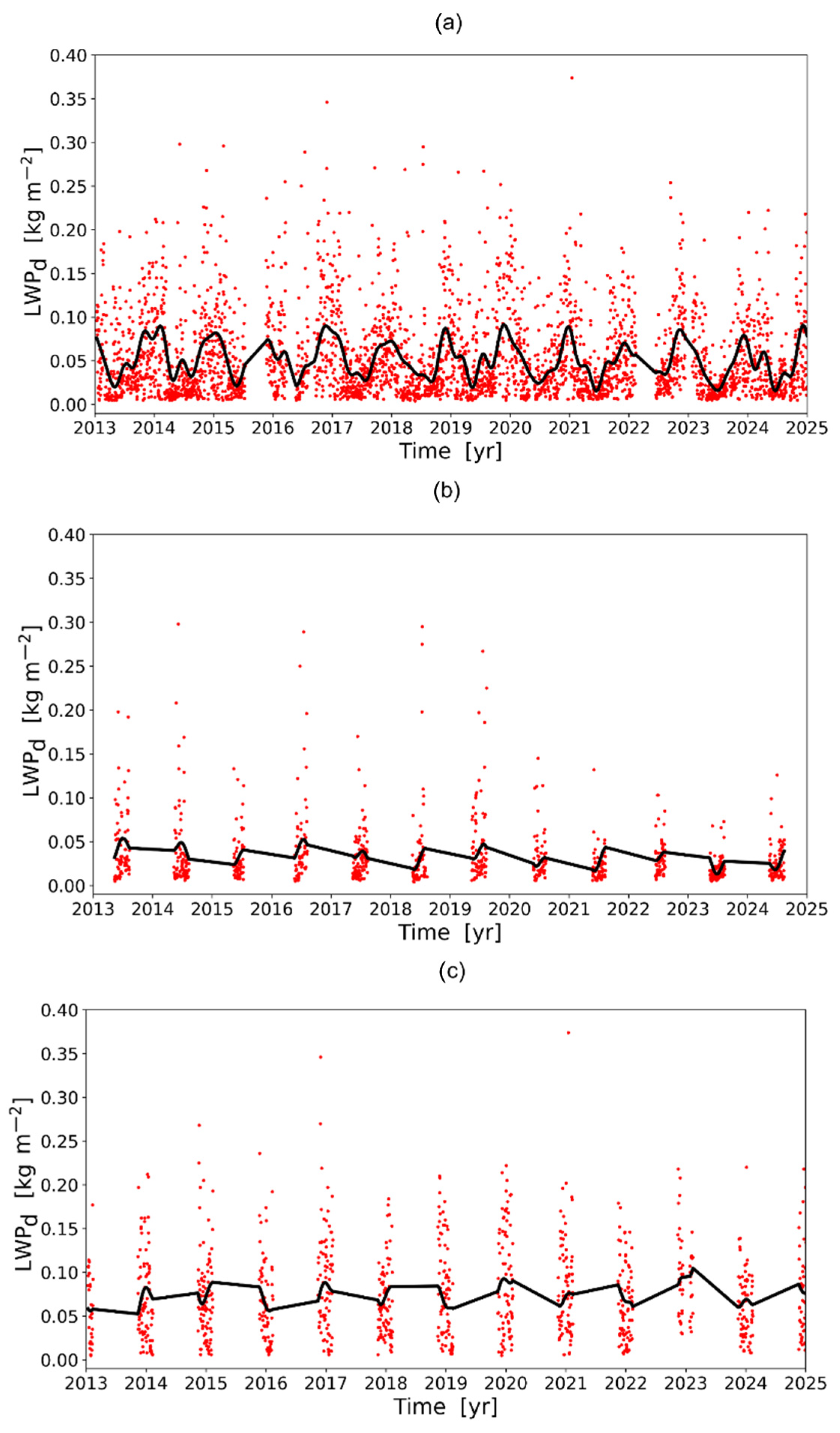
Figure 3a presents the diurnal mean LWP values for the period 2013–2024. One can see that the majority of the data do not exceed 0.2 kg m⁻². One can also notice periodical annual signatures in the data series and two relatively large data gaps in the second half of 2015 and in the first half of 2022. Figure 3b shows the diurnal mean LWP values for the 5-year period without data gaps (2017–2021) and the corresponding running average values where averaging has been performed over 31 days. The following characteristic repeating signatures are marked in the figure as well: (1) several major LWP maxima in late autumn and winter; (2) summer local LWP maximum; and (3) LWP maximum in February-March. Figure 3c gives an impression of the day–night LWP difference by showing the running average of the daytime and the night-time mean values (averaging over 183 days) for the whole considered time period. One can see that from approximately 2013 to 2016, the daytime LWP values are higher than the night-time LWP values, while from 2019 to 2022, the situation is opposite and the night-time LWP values are higher than the daytime LWP values. This feature refers to the diurnal variability, and therefore, it is unlikely a reflection of some long-term instrumental drift. We would like to note that we used running average quantities in order to better detect and identify all specific features of the LWP inter-annual and seasonal behaviour.

4. Trend Assessment on the Basis of Linear Regression and Correlation Coefficient Analysis

The first approach to trend assessment is based on the following simple linear approximation of the annual mean quantities:

$$F(t)=a+bt$$

(6)

where F is the linear approximation function, t is time, and a and b are coefficients that are obtained by the least squares method. The statistical significance of this approximation is determined by the statistical significance of the correlation coefficient. In the case of a relatively large number of samples, the standard deviation of the correlation coefficient can be estimated using the following formula [26]:

$${\sigma }_r\approx {\displaystyle \frac{1-r^2}{\sqrt{n}}}$$

(7)

where r is the correlation coefficient, and n is the number of samples. The correlation relationships between variables and the linear regression coefficient are considered to be statistically significant with confidence levels of 68%, 95%, and 99% when the following corresponding relationships are valid:

$$\left|r\right|\ge {\sigma }_r,\hspace{1em}\left|r\right|\ge 2{\sigma }_r,\hspace{1em}\left|r\right|\ge 3{\sigma }_r$$

(8)

Using expressions (7) and (8), it is easy to construct three quadratic equations and then to derive the minimal correlation coefficients that satisfy the mathematical inequalities (8):

$$r_{68}={\displaystyle \frac{\sqrt{n+4}-\sqrt{n}}{2}};\begin{array}{cc}& \end{array}{r}_{95}={\displaystyle \frac{\sqrt{n+16}-\sqrt{n}}{4}};\begin{array}{cc}& \end{array}{r}_{99}={\displaystyle \frac{\sqrt{n+36}-\sqrt{n}}{6}}$$

(9)

where the subscripts of r denote the confidence level. So, criterion No. 1 for statistical significance of the linear trend with specific confidence levels can be formulated as follows:

$$\left|r\right|\ge r_{68}\hspace{1em}\mathrm{or}\hspace{1em}\left|r\right|\ge r_{95}\hspace{1em}\mathrm{or}\hspace{1em}\left|r\right|\ge r_{99}$$

(10)

For data arrays with small numbers of samples, one might need a stronger criterion. Such a criterion was proposed by Bolshakov [27]. In order to estimate the robustness of a correlation coefficient for a number of data points less than 50, one can use the following function:

$$z={\displaystyle \frac{1}{2}}\left[ln\left(1+r\right)-ln\left(1-r\right)\right]$$

(11)

The values of z are normally distributed with the standard deviation:

$${\sigma }_z={\displaystyle \frac{1}{\sqrt{n-3}}}$$

(12)

For a given value of r, one can calculate the corresponding value of z using Equation (11). Then, the values of the correlation coefficient that correspond to the values z − σ_z and z + σ_z can be obtained by inverting Equation (11):

$$r_1={\displaystyle \frac{exp\left(2(z-{\sigma }_z)\right)-1}{exp\left(2(z-{\sigma }_z)\right)+1}}$$

(13)

$$r_2={\displaystyle \frac{exp\left(2(z+{\sigma }_z)\right)-1}{exp\left(2(z+{\sigma }_z)\right)+1}}$$

(14)

In such a way, the limits of uncertainty of the correlation coefficient r can be estimated:

$$r_1\le r\le r_2$$

(15)

As a result, criterion No. 2 for statistical significance of the linear trend with specific confidence levels can be formulated as follows:

$$r_1\ge r_{68}\hspace{1em}\mathrm{or}\hspace{1em}{r}_1\ge r_{95}\hspace{1em}\mathrm{or}\hspace{1em}{r}_1\ge r_{99}$$

(16)

These relationships are valid for a positive correlation coefficient r₁. For a negative r₁, the minimal absolute value among r₁ and r₂ should be taken instead of r₁. One can see that criterion No. 2 differs from criterion No. 1 by using a smaller value of the correlation coefficient for comparison with the threshold values r₆₈, r₉₅, and r₉₉.

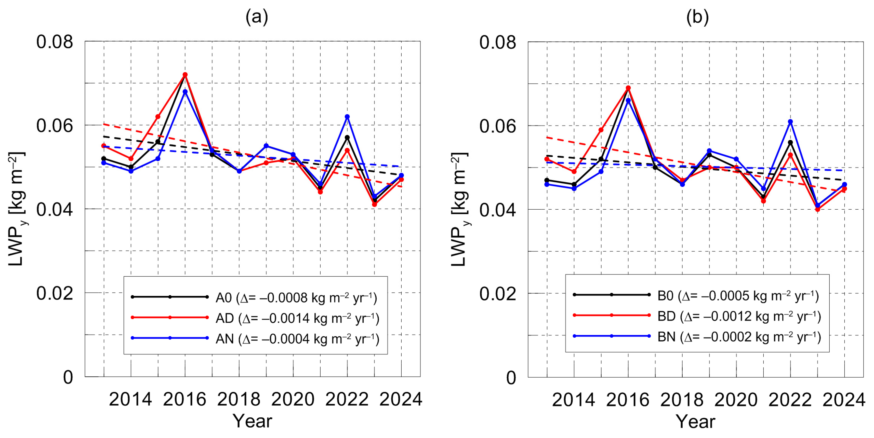
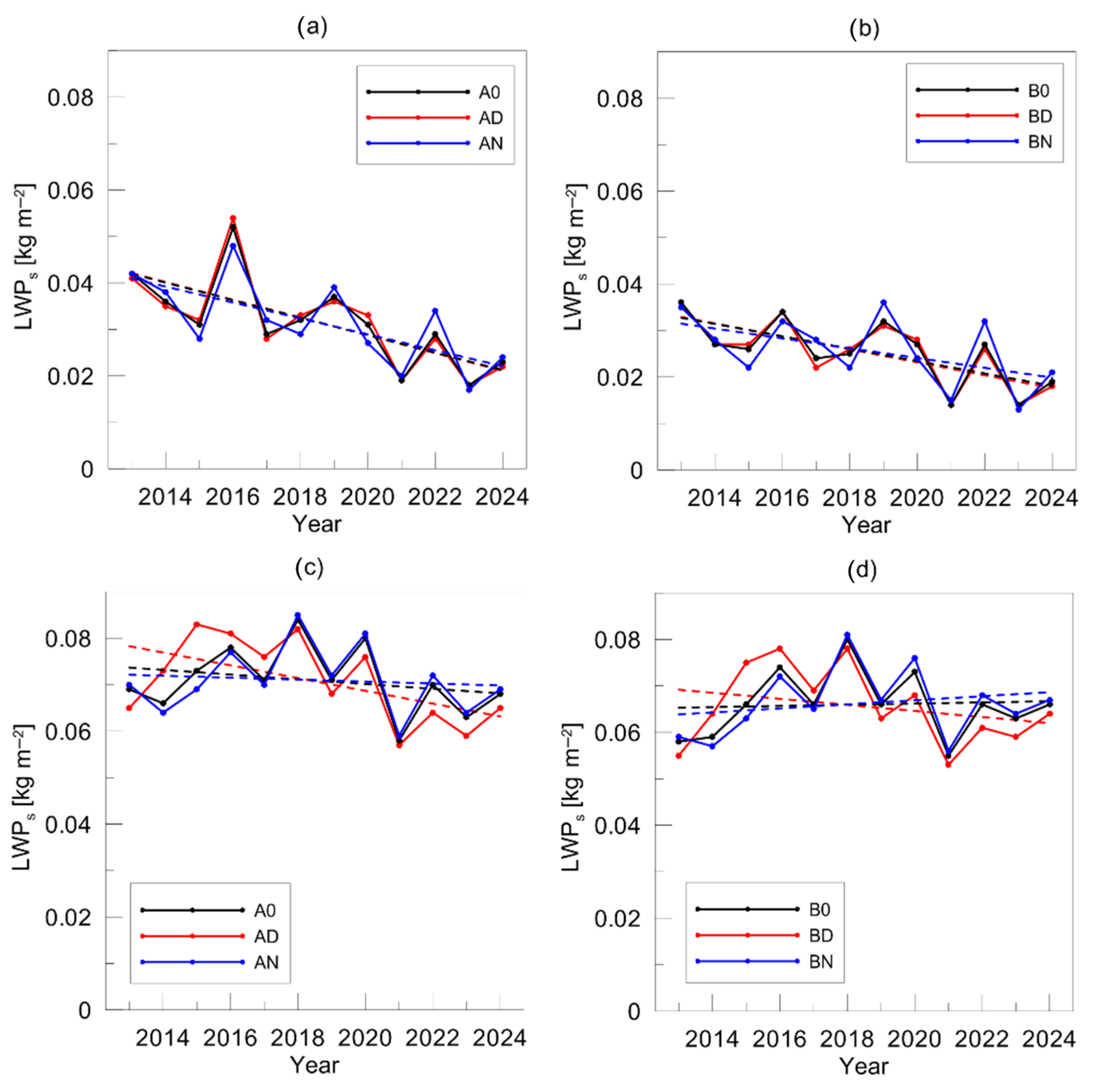
Figure 4 shows the annual mean values of the LWP for the period 2013–2024 calculated for arrays AD, A0, AN, BD, BN, and B0 together with the linear trends that have been obtained by the least squares method. The magnitudes of these trends are presented in the plot legend. As one can see, the daytime values demonstrate maximal absolute values of the trend magnitude: −0.0014 kg m⁻² yr⁻¹ for subset AD and −0.0012 kg m⁻² yr⁻¹ for subset BD. The trend magnitudes for all subsets containing the virtual LWP are smaller than the corresponding trend magnitudes for the true LWP. This fact indicates that the number of clear-sky measurements decreased within the considered period of time. The statistical significance of these trends has been estimated on the basis of correlation coefficient analysis using the two abovementioned criteria. The results of these estimations are presented in

Table 2. Results of assessment of statistical significance of linear trends of annual mean LWP values for the 2013–2024 period (see Figure 4).

Data Subset	Parameter
	n	r68	r95	r99	r	r1	r2	Is Trend Significant?
								Criterion 1	Criterion 2
A0	12	0.27	0.45	0.58	−0.40	−0.64	−0.09	yes, 68%	no
AD					−0.60	−0.77	−0.34	yes, 99%	yes, 68%
AN					−0.23	−0.51	−0.10	no	no
B0					−0.26	−0.54	0.07	no	no
BD					−0.55	−0.74	−0.28	yes, 95%	yes, 68%
BN					−0.09	−0.40	0.24	no	no

. Both criteria confirmed the statistical significance of the linear trends for subsets AD and BD, though with different confidence levels. The trend for A0 is significant according to criterion No. 1. For the night-time true and virtual LWPs and for the all-hour virtual LWP, the trends were not confirmed either by criterion No. 1 or by criterion No. 2.

For the derivation of seasonal trends, we have chosen a three-month period corresponding to a warm season (May, June, July) and a three-month period corresponding to a cold season (November, December, January). Accordingly, trends have been estimated using the three-month mean LWP values calculated for each year within the period 2013–2024. The magnitudes of these trends are given in

Table 3. Magnitudes of all-season general trend and the trends for three-month seasonal LWP values.

Data Subset	Magnitude of the LWP Trend [kg m−2 yr−1]
	All-Season General Trend	Warm Season	Cold Season
A0	−0.0008	−0.0019	−0.00051
AD	−0.0014	−0.0019	−0.0014
AN	−0.0004	−0.0017	−0.00021
B0	−0.0005	−0.0013	0.00013
BD	−0.0012	−0.0014	−0.00065
BN	−0.0002	−0.0011	0.00044

together with the magnitudes of the all-season general trend. The results of the estimations of statistical significance are presented in

Table 4. Results of assessment of statistical significance of linear trends of LWP values for a warm season during the 2013–2024 period (see Table 3).

Data Subset	Parameter
	n	r68	r95	r99	r	r1	r2	Is Trend Significant?
								Criterion 1	Criterion 2
A0	12	0.27	0.45	0.58	−0.71	−0.84	−0.50	yes, 99%	yes, 95%
AD					−0.69	−0.83	−0.48	yes, 99%	yes, 95%
AN					−0.67	−0.82	−0.45	yes, 99%	yes, 95%
B0					−0.68	−0.82	−0.47	yes, 99%	yes, 95%
BD					−0.71	−0.84	−0.50	yes, 99%	yes, 95%
BN					−0.51	−0.72	−0.23	yes, 95%	no

and

Table 5. Results of assessment of statistical significance of linear trends of LWP values for a cold season during the 2013–2024 period (see Table 3).

Data Subset	Parameter
	n	r68	r95	r99	r	r1	r2	Is Trend Significant?
								Criterion 1	Criterion 2
A0	12	0.27	0.45	0.58	−0.25	−0.53	0.07	no	no
AD					−0.55	−0.74	−0.28	yes, 95%	yes, 68%
AN					−0.10	−0.41	0.23	no	no
B0					0.06	−0.26	0.38	no	no
BD					−0.28	−0.55	0.04	yes, 68%	no
BN					0.21	−0.12	0.50	no	no

. One can see the evident differences between the results for a warm and for a cold period for most data subsets. The absolute values of the magnitudes of trends for a warm period are much larger than for a cold period. Thus, Table 3 shows that the trend values for subset B0 and different seasons differ by one order of magnitude. Moreover, the trend for B0 and a cold season is positive (0.00013 kg m⁻² yr⁻¹), while the trend for a warm season is negative (−0.0013 kg m⁻² yr⁻¹). For other data subsets, except AD, the absolute values of the trend magnitudes differ by factors from 2 to 8. Therefore, for a cold period, there is only one subset—AD—for which the trend can be called noticeable (−0.0014 kg m⁻² yr⁻¹) and comparable to the trend for a warm season (−0.0019 kg m⁻² yr⁻¹), while for other subsets, the absolute values of the trend magnitudes for a cold season are negligibly small. A comparison of Table 4 and Table 5 shows that the number of statistically significant trends for a warm season is much larger than for a cold season. This is the result of the differences between the values of the correlation coefficients for a warm and for a cold season. For a warm season, the correlation coefficients r are in the range from −0.71 to −0.51, while for a cold season, the correlation coefficients r are in the range from −0.55 to 0.06. As can also be seen from Table 4, the trends corresponding to a warm season are statistically significant according to both criteria for all subsets except subset BN. For subset BN, the stronger criterion No. 2 has not been satisfied. In contrast to a warm season, the trends for a cold season are significant only for two data subsets: AD and BD (see Table 5). However, it should be emphasised that for subset BN, the confidence level is low: only 68%.

Concluding this section, we present the plot that illustrates the differences between the trends of the LWP for a warm and for a cold season. Figure 5 shows the 3-month mean values of the LWP for a warm period and for a cold period as defined above and calculated for each year within the time interval 2013–2024. The mean values are shown for data subsets AD, A0, AN, BD, BN, and B0 together with the linear trends that have been obtained by the least squares method. The magnitudes of these trends are given in Table 3 and have been already discussed. We would just like to add that similar to the results of the assessment of the general trends shown above, smaller seasonal trends are detected for all subsets containing the virtual LWP (mixed clear-sky and cloudy cases) if compared to true LWP seasonal trends. This fact indicates that the number of clear-sky measurements during both seasons decreased within the considered period of time.

5. Trend Assessment on the Basis of the Lomb–Scargle Method with Cross-Validation and Bootstrapping Techniques

The second approach to trend assessment that we used in the present study is mainly based on the Lomb–Scargle analysis. It is a modification of Fourier analysis for uneven time series [28,29,30]. A cross-validation technique provides the opportunity to check whether the chosen fitting model is optimal. The reliability of the obtained long-term trends is evaluated by the so-called “statistical bootstrapping”. The description of this original combined approach can be found in the study by Makarova et al. [31] in which the trends of several important greenhouse gases in the atmosphere have been obtained from the 14-year series of ground-based remote spectroscopic measurements. Here, we briefly present the main steps and ideas of the combined approach. At the initial step, the assumption is made that the data series can be approximated by a model function F(t):

$$F(t)=a+bt+{\displaystyle \sum _{i=1}^N{c}_{i}Cos({\alpha }_{i}t+{\varphi }_i)}$$

(17)

where t is time; N is the number of harmonic functions; and a, b, c_i, α_i, and φ_i are the coefficients to be determined. This assumption is typical and widely used for the analysis of time series of atmospheric trace gases [32]. Obviously, the long-term trend of the analysed quantity is equal to the coefficient b, which characterises the slope of the linear function. In order to obtain statistical characteristics (the mean value of b, the confidence levels, and the uncertainty of b), we performed the following steps:

(1)

Preliminary detrending of data series has been achieved using simple linear regression.

(2)

After detrending, the Lomb-Scargle method is applied to the data. The outcome is a set of n periods/frequencies having peaks (maxima) of spectral density in a periodogram.

(3)

An optimal subset of N harmonic functions is derived from the full set of n functions. To achieve this goal, we applied the cross-validation technique. The relevant procedure involves dividing the available time series into multiple subsets, using one of these subsets as a validation set, and training the model on the remaining subsets (https://www.geeksforgeeks.org/cross-validation-machine-learning/). We made this analysis multiple times, including i most significant harmonic functions at each step (starting from i = 1 and ending with i = n). For each step, we determined the root mean square (RMS) value of the discrepancy between the validation set and the model function F(t). The optimal number N provides minimum value of the RMS discrepancy between the model and the validation set.

(4)

At the final step, the mean value of a trend (coefficient b) and its confidence intervals and uncertainty are evaluated. For this purpose, the bootstrapping approach was implemented [32,33], with a bootstrap population of ~400 (a further increase in this number does not lead to any noticeable changes in the results).

At all stages, the data fitting was performed by the least squares method. As a result, we obtained the optimal number of harmonics N and the minimal (S_min), maximal (S_max), and mean (S_mean) values of the trend magnitude and its standard deviation (σ_s). These quantities are derived from an ensemble of trend magnitudes that is constructed during the bootstrapping procedure. The statistical significance of a trend is estimated by comparing the quantities S_mean and σ_s. A trend is considered to be statistically significant with confidence levels of 68%, 95%, and 99% when the following corresponding relationships are valid:

$$\left|S_{mean}\right|\ge {\sigma }_s\begin{array}{cc},& \end{array}\left|S_{mean}\right|\ge 2{\sigma }_s\begin{array}{cc},& \end{array}\left|S_{mean}\right|\ge 3{\sigma }_s$$

(18)

The Lomb–Scargle combined method has been applied to the diurnal mean LWP time series.

Table 6. Magnitudes of linear trends and corresponding standard deviations obtained for full time series (all seasons) for subsets A0, AD, AN, B0, BD, and BN.

Data Subset	Number of Harmonics	Magnitude of the Trend [kg m−2 yr−1]			Standard Deviation [kg m−2 yr−1]	Is Trend Significant?
		Min	Max	Mean
A0	3	−0.0013	−0.00041	−0.00064	0.00015	yes, 99%
AD	2	−0.0017	−0.00082	−0.0011	0.00015	yes, 99%
AN	3	−0.00088	−0.000014	−0.00032	0.00015	yes, 95%
B0	3	−0.0011	−0.00019	−0.00042	0.00017	yes, 95%
BD	2	−0.0015	−0.00064	−0.00094	0.00014	yes, 99%
BN	2	−0.00082	0.00020	−0.00015	0.00018	no

presents the estimation of the trend magnitudes for different subsets of full time series. The trends are statistically significant for all subsets with confidence levels higher than 95% except for subset BN. For subset BN, the trend is not significant even at the lowest confidence level of 68%.

Table 7. Magnitudes of linear trends and corresponding standard deviations obtained for a warm season for subsets A0, AD, AN, B0, BD, and BN.

Data Subset	Number of Harmonics	Magnitude of the Trend [kg m−2 yr−1]			Standard Deviation [kg m−2 yr−1]	Is Trend Significant?
		Min	Max	Mean
A0	3	−0.0017	−0.0010	−0.0013	0.00012	yes, 99%
AD	2	−0.0020	−0.00091	−0.0014	0.00015	yes, 99%
AN	3	−0.0017	−0.00091	−0.0012	0.00012	yes, 99%
B0	3	−0.0014	−0.00076	−0.0011	0.00013	yes, 99%
BD	2	−0.0017	−0.00058	−0.00095	0.00022	yes, 99%
BN	2	−0.0015	−0.00063	−0.00099	0.00013	yes, 99%

and

Table 8. Magnitudes of linear trends and corresponding standard deviations obtained for a cold season for subsets A0, AD, AN, B0, BD, and BN.

Data Subset	Number of Harmonics	Magnitude of the Trend [kg m−2 yr−1]			Standard Deviation [kg m−2 yr−1]	Is Trend Significant?
		Min	Max	Mean
A0	3	−0.000088	0.0014	0.00062	0.00023	yes, 95%
AD	2	−0.0012	−0.000097	−0.00064	0.00026	yes, 95%
AN	3	−0.00026	0.0017	0.00073	0.00037	yes, 68%
B0	3	−0.00016	0.0014	0.00079	0.00030	yes, 95%
BD	2	−0.00075	0.00059	0.000068	0.00026	yes, 95%
BN	2	0.000024	0.0017	0.00098	0.00033	yes, 95%

present the trend magnitudes for a warm season and for a cold season. For a warm season, all trends are negative, and all of them are statistically significant with a confidence level of 99%. In contrast, for a cold season, only one of the trends is negative (subset AD). The trends for other data subsets for a cold season are positive. It should be emphasised that the absolute values of the trend magnitudes for a cold season are noticeably smaller than for a warm season. All trends for a cold season, however, are statistically significant with a confidence level of 68–95%. A comparison of the trend magnitudes obtained in the present study by the two approaches is presented below in the Section 6.

Finally, as an illustration of the processing of the data series by the Lomb–Scargle combined method, we present Figure 6. In this figure, the time series of the diurnal LWP (subsets A0) are shown together with the corresponding approximations by Equation (16). The plots in this figure are vivid examples how the combined approach works for time series with data gaps of different sizes. The all-season series has only two noticeable data gaps in 2015 and 2022 lasting for several months. Seasonal time series are characterised by periodical gaps of nine months every year. Nevertheless, there is good agreement between the trends for all seasons and for specific seasons. The largest and the smallest trends are observed for a warm and for a cold season, respectively, and the all-season trend is of medium magnitude. This agreement has already been demonstrated by the results obtained by the first approach to trend assessment.

6. Discussion

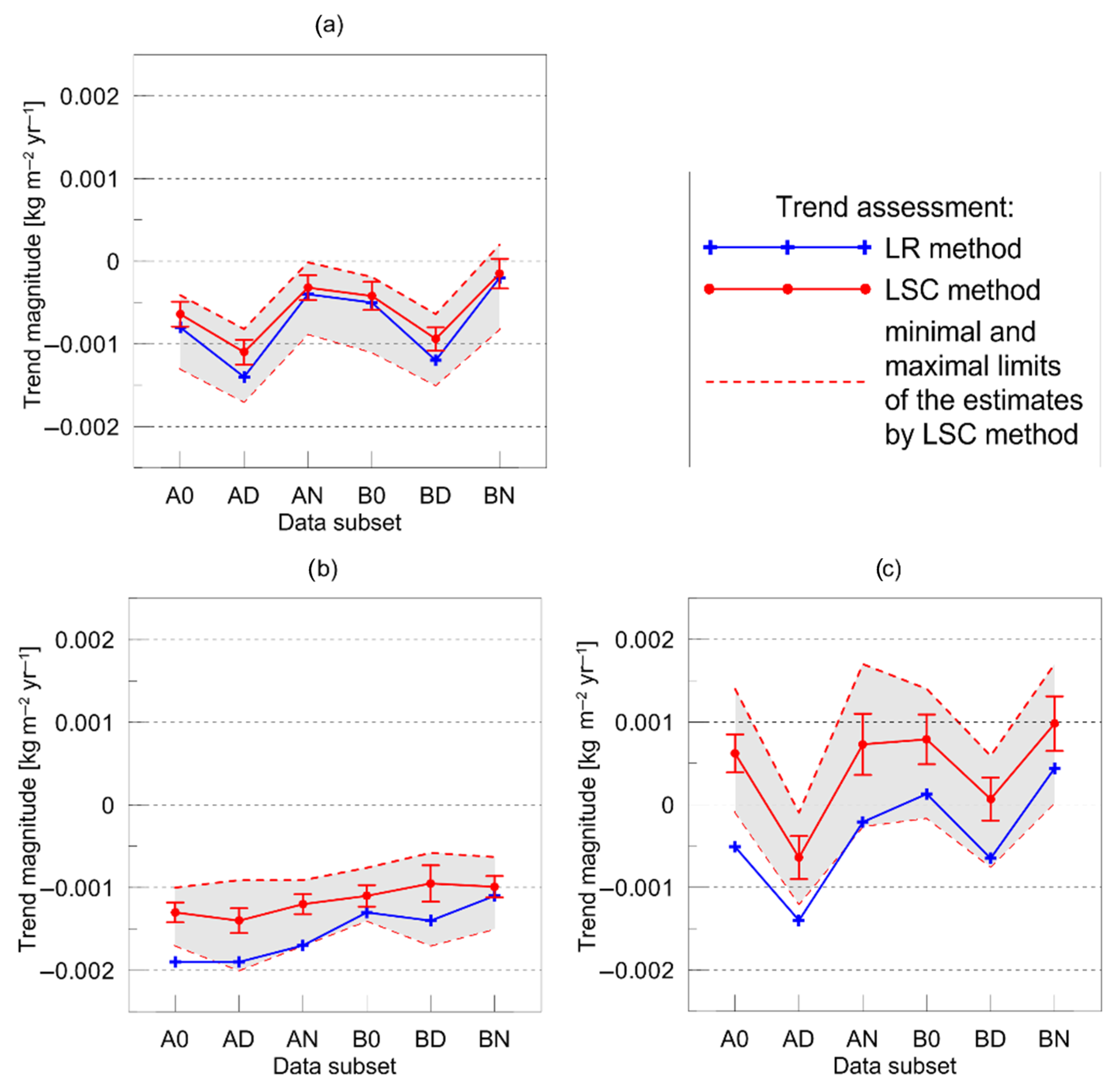
Figure 7 illustrates the comparison of the trend magnitudes obtained in the present study by two different methods. For convenience, we will use the abbreviation LR for the linear regression and correlation analysis method and the abbreviation LSC for the Lomb–Scargle combined method. The comparison has been made for all data subsets and for three time series corresponding to all seasons, to a warm season, and to a cold season. The LSC method provides the estimates of the standard deviation σ_s of the trends, and these estimates are shown in Figure 7 as error bars. It should be noted that the range of 3σ_s coincides well with the shaded areas that designate the range between the minimum and maximum trend estimates obtained by the LSC method.

First of all, we note an excellent agreement of the results obtained by the two methods for the all-season time series. For all subsets, the differences between the trend magnitudes obtained by the LR and LSC methods do not exceed σ_s or 2σ_s. Both methods revealed maximal absolute values of trend magnitudes for subsets AD and BD and minimal values for subsets AN and BN. If we compare the subset pairs A0-B0, AD-BD, and AN-BN, we notice that both methods demonstrate the same feature: the absolute values of the trend magnitudes for the B-subsets are smaller than for the A-subsets. This is a very important result that points at the decrease in the number of clear-sky measurements within the period 2013–2024. It should be noted that the absolute values of the trend magnitudes derived by the LR method are systematically higher than the ones derived by the LSC method.

Both methods show that the maximal absolute values of the trend magnitudes are observed for a warm season time series (Figure 7b). For a warm season, the agreement between the results obtained by the two methods for B-subsets is within the range of σ_s or 2σ_s. The agreement for A-subsets is within the range of 3σ_s. The absolute values of the trend magnitudes derived by the LR method are systematically higher than the ones derived by the LSC method, and this systematic difference for a warm season time series is noticeably larger than the difference for the all-season time series.

The largest discrepancies between the results obtained by the two methods as well as the largest standard deviations σ_s are detected for a cold season time series. Nevertheless, the results agree within the range of 3σ_s. It should be emphasised that for this time series, the trend magnitudes are closer to zero, and the trends for different data subsets differ by sign. One can come to the conclusion that for a cold season time series, the trends are very uncertain despite the fact that the LSC method has confirmed their statistical significance.

So, the obtained above results point at significant negative cloud LWP trends in the vicinity of the Gulf of Finland within the period 2013–2024. First of all, it should be emphasised that these trends are the intrinsic features of clouds, since the largest trends are detected for true LWP data subsets (A-subsets), which do not contain clear-sky measurements. Moreover, the smaller trends for virtual LWP subsets (B-subsets), which contain cloudy and clear-sky LWP measurements together, are an indication of the fact that the number of clear-sky cases decreases in the course of the 2013–2024 period of time. We are reminded that the virtual LWP characterises the atmosphere as a whole, i.e., as a system with or without clouds. The second important finding is the strong seasonal dependence of the trends: one can see that the all-season trends are stipulated mainly by warm season trends, while the cold season trends are small, have a changing sign, and are much more uncertain.

We do not have at our disposal any independent estimates of LWP trends in the vicinity of the Gulf of Finland for the period 2013–2024 to compare with our results. Therefore, we outline only some general considerations relevant to the observed LWP trend magnitudes and the seasonal dependences of trends over the globe and over Europe. The LWP trends on the global scale over oceans and other water bodies have been derived in studies by Manaster et al. [18] and Elsaesser et al. [17] for the time period 1988–2014 (2016) from satellite microwave observations. Global maps of these trends demonstrate a considerable variability in sign and in magnitude depending on geographic location. The trend magnitudes vary from −10 g m⁻² decade⁻¹ to 10 g m⁻² decade⁻¹ (using our notation: from −0.001 kg m⁻² yr⁻¹ to 0.001 kg m⁻² yr⁻¹). One can see that these estimations agree very well with our results for the all-season data subsets and for the cold season data subsets.

The results of the study by Devasthale et al. [34] showed a strong correlation of the surface incoming solar radiation (SIS) with the daytime cloud fraction and with the liquid cloud optical thickness (COT). However, one should keep in mind that there is a strong spatio-temporal variability in these correlations. Since the COT is linked to the LWP, one can expect a strong correlation between the SIS and LWP. So, there is the possibility of indirectly assessing the LWP trends on the basis of the observed SIS trends. Devasthale et al. [34] examined the recent trends in SIS (1988–2020) and cloud properties and found a large-scale increase in the SIS over much of Europe during the spring and early summer. They have shown that this SIS increase is accompanied by large-scale decreases in the daytime cloud fraction and cloud opacity. The most striking increases in the SIS over Central and Eastern Europe reaching more than 6 W/m²/decade over southern Scandinavia, Germany, Switzerland, Italy, Belarus, Ukraine, and western Russia are detected in June. These findings are in good agreement with the results of the present study, which point to the warm season (May–July) as the season of maximal (by absolute value) negative trends. However, the comparison of the true LWP and virtual LWP trends in our study leads to the conclusion that the contribution of clear-sky episodes (in other words, the contribution of the cloud fraction) to the trends is much smaller than the contribution of the direct decrease in the cloud water content (in other words, the decrease in COT). This conclusion is based on the fact that the difference between the trend magnitudes of the true and virtual LWPs is not large. Moreover, if we take into account that the trends of the true and virtual LWPs are similar and negative but the trend magnitude of the virtual LWP is less (by absolute value) than the trend magnitude of the true LWP, we can conclude that the number of clear-sky cases has been decreasing within the analysed period of time. Obviously, clear-sky cases modify the LWP trend. Let us consider a simple example when the true LWP trend is equal to zero. If the number of clear-sky cases increases/decreases in time, then we will obtain the negative/positive virtual LWP trend while there will be no true LWP trend. 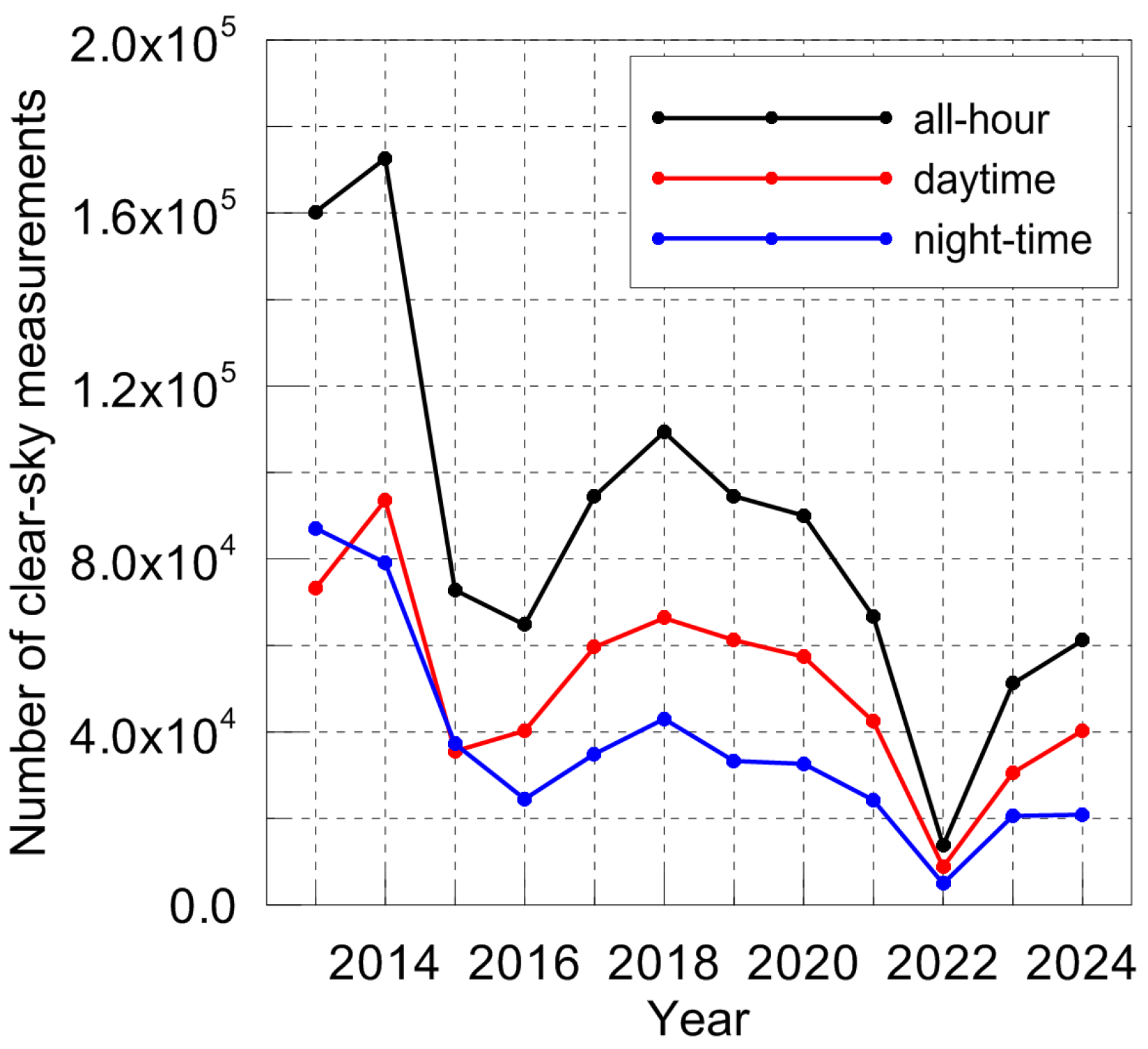Figure 8 shows the total number of clear-sky measurements per year within the considered period of time. One can see that the number of clear-sky measurements decreased approximately by a factor of 4 if the years 2013 and 2024 are compared. This reduction resulted in a larger relative number of cloudy cases, which produced a weaker trend of the virtual LWP if compared to the trend of the real LWP. An interesting feature is the larger number of clear-sky measurements in the daytime than at night practically for all years of observations except 2013–2015 when these quantities are close to each other.

Since we used two different methods for LWP trend assessment, it is necessary to choose which results can be considered as the final results of this study. Both methods are rigorous and reliable, but in our opinion, the Lomb–Scargle combined method provides more information for comprehensive analysis, including direct estimations of the standard deviation of the trend magnitude. Moreover, one must take into account the fact that the results of the LR method are based on a relatively small number of sample data. Therefore, in our conclusions, we present the results of the LSC method as the basic and final ones.

Concluding this section, we would like to note that to the best of our knowledge, our study is the first one to present the analysis of long-term, high-accuracy, ground-based measurements of the cloud LWP by the microwave method in Northern Europe. The high accuracy of the initial data should be especially emphasised. Satellite measurements of the LWP contain larger errors, and it is well-known that ground-based microwave measurements of the LWP are taken as a reference in many studies relevant to the validation of satellite data. We believe that our results may be valuable for the validation of long-term trends derived from the satellite data. Furthermore, there is still the problem of modelling the LWP trends: as an example, we point out the study by Manaster et al. [18] in which it has been shown that for many regions over oceans, the LWP trend magnitudes observed from space by passive microwave sounders can be up to four times larger than the corresponding model mean trend magnitudes. We present this general example since we are not aware of any studies focusing on the LWP trend analysis in the very geographical area that is considered in our work. We believe that the trends obtained in our study may be useful for the development of regional climate models in Northern Europe.

7. Summary and Conclusions

In the present study, the linear trends of the cloud liquid water path are assessed on the basis of the 12-year (2013–2024) time series of LWP values obtained from the microwave observations by the RPG-HATPRO radiometer located at about 2.5 km from the coastline of the Gulf of Finland (59.88107° N, 29.82597° E). All estimations have been conducted for LWP values smaller than 0.4 kg m⁻² since this value has been reported earlier as a threshold LWP between non-rainy and rainy atmospheres. The two major types of data subsets are “A”, which contain measurements under cloudy conditions only, and “B”, which contain mixed clear-sky measurements and measurements under cloudy conditions. We use the term “true LWP” for the LWP in “A”-subsets and the term “virtual LWP” for the LWP in “B”-subsets, since we assign a zero LWP value to clear-sky measurements. “A”-subsets describe the intrinsic properties of clouds, while “B”-subsets describe the atmosphere with and without clouds “as a whole”. Additional sorting of the data has been performed depending on the solar zenith angle in order to study the diurnal features of the LWP (all-hour, daytime, and night-time).

Two approaches have been used for trend assessment. The first approach is based on the linear regression and correlation coefficient analysis (LR method), and it is used for processing annual mean quantities. The second approach is based on the combination of the Lomb–Scargle method with the cross-validation and bootstrapping techniques (LSC method), and it is used for processing the time series of diurnal mean quantities. Both methods provide the trend magnitude and the level of its statistical significance. In addition, the LSC method provides the standard deviation of the trend magnitude. A comparison of the results of the trend magnitude estimations obtained by the two methods has shown good agreement within the error limits. The results of the LSC method are adopted as the basic and final ones due to two reasons: first, the LSC method provides more information for comprehensive analysis, and second, the results of the LR method are based on a relatively small number of sample data.

In the course of this study, the following main results of the LWP trend assessment for the period 2013–2024 have been obtained:

(1)

The trends for all subsets of data are statistically significant except for the general (all-season) night-time trend of the virtual LWP. The level of significance is higher than 95% for all subsets except the subset containing the true night-time LWP (68%).

(2)

The most pronounced general trend of the LWP over the period 2013–2024 has been detected for the daytime true LWP, and it constitutes −0.0011 ± 0.00015 kg m⁻² yr⁻¹. This trend is driven mainly by the daytime true LWP trend for a warm season (May-July, −0.0014 ± 0.00015 kg m⁻² yr⁻¹), which is considerably larger than the daytime trend for a cold season (November-January, −0.00064 ± 0.00026 kg m⁻² yr⁻¹).

(3)

Comparison of the true and virtual LWP trends points to a decrease in the number of clear-sky measurements over the period 2013–2024. The analysis has shown that the number of clear-sky measurements decreased approximately by a factor of 4 if years 2013 and 2024 are compared. Additionally, our study has revealed that the contribution of clear-sky episodes to the trends of the virtual LWP is much smaller than the contribution of the direct decrease in the cloud water content.

(4)

The LWP trend magnitudes obtained in the present study are in good agreement with the global-wide estimations of the range of LWP trends, which are from −0.001 kg m⁻² yr⁻¹ to 0.001 kg m⁻² yr⁻¹. Furthermore, the results of the present study point at the warm season (May-July) as the season with the maximal (by absolute value) negative trends of the LWP. This finding is in a good agreement with a report by Devasthale et al. [34] showing a striking increase in surface incoming solar radiation over Central and Eastern Europe detected in June.