Aerosol, Clouds and Radiation Interactions in the NCEP Unified Forecast Systems

Abstract

In this study, we evaluate aerosol, cloud, and radiation interactions in GFS.V17.p8 (Global Forecast System System Version 17 prototype 8). Two experiments were conducted for the summer of 2020. In the control experiment (EXP CTL), aerosols interact with radiation only, incorporating direct and semi-direct aerosol effects. The sensitivity experiment (EXP ACI) couples aerosols with both radiation and Thompson microphysics, accounting for aerosol indirect effects and fully interactive aerosol–cloud dynamics. Introducing aerosol and cloud interactions results in net cooling at the top of the atmosphere (TOA). Further analysis shows that the EXP ACI produces more liquid water at lower levels and less ice water at higher levels compared to the EXP CTL. The aerosol optical depth (AOD) shows a good linear relationship with cloud droplet number concentration, similar to other climate models, though with larger standard deviations. Including aerosol and cloud interactions generally enhances simulations of the Indian Summer Monsoon, stratocumulus, and diurnal cycles. Additionally, the study evaluates the impacts of aerosols on deep convection and cloud life cycles.

1. Introduction

Aerosols—such as dust, carbon, sulfate, and sea salt—significantly impact net radiation both at the top and bottom of the atmosphere and influence cloud–radiation interactions. One key effect of the aerosol–radiation interaction is the aerosol direct effect (ADE, e.g., [1,2]. ADE involves the scattering or reflection of solar radiation by aerosols, leading to reduced solar radiation reaching the ground (known as dimming effects). This typically results in cooling of the atmosphere and Earth system. The dimming effects can cause surface cooling, reduced latent and sensible heat fluxes, and decreased global precipitation. Conversely, the semi-direct effect arises when aerosols, such as black carbon, absorb solar radiation, which can increase the temperature of the system e.g., [3]. In numerical models, it is essential to couple aerosols with radiation to accurately represent the ADE.

Another key effect of aerosol–cloud–radiation interactions is the aerosol indirect effect (AIE, [4]). AIE involves aerosols altering cloud properties by modifying the number of cloud droplets or particles, their effective radius (Re), and cloud water content through the activation of cloud condensation nuclei (CCN) and ice nuclei (IN). To accurately represent AIE in numerical models, it is essential to couple aerosols with microphysics. AIE is typically categorized into two types: the first indirect effect and the second indirect effect. The first indirect effect occurs when increased aerosol concentration leads to a higher number of cloud and ice water droplets, enhancing cloud albedo. The second indirect effect results from the reduction in cloud droplet or particle size, which affects precipitation efficiency and cloud lifetime e.g., [5].

Although observations are subject to measurement uncertainty and model studies are constrained by computational resources and the limits of fundamental physical process parameterizations, both models (e.g., [6,7,8,9,10,11]) and observations (e.g., [12]) have provided insights into deep convection invigoration by aerosol loading. Increased aerosol concentrations can lead to smaller but more numerous cloud droplets and ice crystals through cloud and ice nucleation processes. This, in turn, affects the cloud’s horizontal and vertical extent, optical depth, liquid water path, and even lightning activity when coupled with dynamic processes. The effects of aerosols on surface precipitation and cloud system life cycles are complex and may show a negative correlation with precipitation and cloud system lifespan. Aerosols can suppress warm-rain processes, enhance supercooled droplet formation aloft, increase glaciation from supercooled droplets, and promote graupel and hail production through riming processes, which release additional latent heat. Consequently, there is often little or no invigoration in warm clouds.

Some studies present contrary findings to aerosol invigoration of cloud systems (e.g., [13,14]) or suggest a neutral effect (e.g., [15,16,17,18]). Khain (2009) [16] and Altaratz et al. (2014) [15] provide a comprehensive summary of this apparent confusion and the conflicting effects, which stem from the use of an “ideal” invigoration cloud system. Typically, this system is characterized by deep convection in relatively highly unstable and humid environments with little to no vertical wind shear.

The effects of aerosols on atmospheric temperature and climate over South Asia are increasingly being studied through both regional and global climate models and observations. The elevated heat pump (EHP) effect, proposed by Lau et al. (2008) [19], suggests that the heating effects of black carbon and dust over the southern slopes of the Tibetan Plateau create a positive temperature anomaly in the mid- to upper-troposphere relative to the region to the south. This temperature anomaly drives hot air upward, drawing in additional warm and moist air over the Indian Peninsula and strengthening the circulation that leads to the early onset and intensification of the Indian monsoon. However, Guo et al. (2016) [18] noted significant uncertainties related to black carbon (BC) emissions, which need to be scaled up to accurately assess the associated rainfall increases over northern India. Evidence from Ramanathan et al. (2001) [20] and Bollasina et al. (2011) [21] highlights how aerosols influence regional climate changes, including reductions in cloudiness (e.g., [22]) and alterations in precipitation patterns (e.g., [23]), through their direct, semi-direct, and indirect effects on the hydrological cycle and tropical meridional overturning circulation.

There is relatively limited research on aerosol, radiation, and cloud interactions using operational numerical weather prediction (NWP) models. NWPs typically have horizontal grid spacings around 10 km, placing them in the gray zone where interactions between aerosols and clouds may be less parameterized compared to climate models. Additionally, NWPs are heavily tuned for optimal forecasting performance, which means aerosol loading in the default settings may reflect current real-world conditions, leading to further complexities in studying aerosol–cloud interactions (ACIs) in these models.

The Copernicus Atmosphere Monitoring Service (CAMS) integrated into the ECMWF Integrated Forecasting System (IFS) has shown that the more reflective dust from CAMS affects the northeast branch of the Indian monsoon by altering the temperature gradient. This improvement in the temperature, zonal wind, and precipitation over the Indian Ocean and western India results in about a 30% reduction in model errors ([24]). Using the Global Forecast System (GFS) of the Unified Forecast System (UFS), Cheng and Yang (2023) [25] found that aerosol radiative forcing over the Arabian and Indian Peninsulas causes cooling in the lower troposphere (dimming effects) and warming in the upper troposphere (absorbing effects). They found that replacing the default aerosol dataset with MERRA2 data slightly strengthens the northward monsoonal flow over the western and southern Indian subcontinent. Similar work has been conducted using forecasted aerosols with a low-resolution GFS by Zhang et al. (2022) [26]. An interesting finding is that comparable aerosol–radiation interaction (ARI) effects and model performance were observed on weekly and monthly scales, aligning with the results of Cheng and Yang (2023) [25]. Mulcahy et al. (2014) [27] included indirect aerosol effects from prognostic aerosols and found that changes in cloud droplet number concentration (CDNC) dominate in South Asia, rather than direct absorption by aerosols. This finding contrasts with [19], suggesting that missing aerosol sources or an underestimation of absorbing aerosol optical properties may be contributing factors, warranting further investigation.

In this study, we first investigate aerosol, cloud, and radiation interactions in the UFS model and compare these interactions with available satellite observations and other models. We examine the regional impacts of aerosol effects on circulation within the Indian monsoon region and conduct a series of single column model (SCM) experiments to assess aerosol indirect effects. The use of SCM is motivated by its ability to replay the online UFS simulations, which simplifies the analysis and enhances our understanding of the physical processes involved. The Common Community Physics Package-SCM (CCPP-SCM) shares the same code as GFS.V17.p8 and is synchronized with the latest GFS updates. This ensures that all physics processes, including radiation and cloud dynamics, are consistent with GFS.V17.p8. Moreover, the CCPP-SCM used in this study can reproduce GFS.V17.p8 results byte-for-byte by utilizing initial conditions and forcing derived output from GFS.V17.p8. Additionally, we study the influence of aerosols on stratocumulus clouds and the diurnal cycle using the CCPP-SCM. To isolate the effects of aerosols on storm system life cycles and aerosol invigoration, we have selected a site with minimal horizontal advection.

The remainder of the paper is structured as follows: Section 2 outlines the experimental design, followed by the presentation of results in Section 3. Finally, Section 4 provides a summary and conclusions.

2. Experimental Design and Model Description

For this study, we utilize the GFS version 17 prototype 8 (GFS.V17.p8) [28], which features a horizontal resolution of approximately 13 km and 127 vertical levels extending to the mesopause (C768L128 GFS). Additionally, data from specific locations extracted from the GFS are used to drive the CCPP Single Column Model (SCM). The operational implementation of GFS.V17 is scheduled for March 2025. This version employs Thompson microphysics ([29,30]) and the Rapid Radiation Transfer Model for GCM [31,32,33].

The Modern-Era Retrospective analysis for Research and Applications, Version 2 (MERRA2; [34,35]) aerosol climatology was employed to drive radiation processes [25] and was coupled with Thompson microphysics in all experiments. The study incorporates five bins each for dust and sea salt, two bins for black carbon and organic carbon, and one bin for sulfate aerosols. Secondary aerosol formation is excluded from this setup.

Thompson microphysics, a double-moment scheme, predicts and advects both the mixing ratios and number concentrations of condensates and hydrometeors. However, for computational efficiency, the version used in this study does not predict the number concentrations of snow and graupel. The activation of ice nuclei (IN) and cloud condensation nuclei (CCN) depends on the Number concentrations of Ice-Friendly Aerosols (NIFA, [36]) and Water-Friendly Aerosols (NWFA, Thompson and Eidhammer, 2014), respectively. A look-up table is employed for CCN activation, based on NWFA, vertical velocity (w), temperature (T), mean aerosol radius, and hygroscopic parameters (details are provided in the Appendix A). This table was generated using Köhler activation theory within a parcel model by Feingold and Heymsfield (1992) [37], explicitly considering these five variables. NIFA and NWFA are calculated as below:

$$\mathrm{N}\mathrm{I}\mathrm{F}\mathrm{A}={\displaystyle \frac{m{r}_{du1}}{m_{du1}}}+{\displaystyle \frac{{mr}_{du2}}{m_{du2}}}+{\displaystyle \frac{{mr}_{du3}}{m_{du3}}}+{\displaystyle \frac{m{r}_{du4}}{m_{du4}}}+{\displaystyle \frac{m{r}_{du5}}{m_{du5}}}$$

where mr is the mixing ratio for each dust bin, subscript du1 represents dust bin 1, and m is the mass for each particle in the bin. $m={\displaystyle \frac{4}{3}}\pi r^3\rho$. $\rho$ is the density and r is the medium radius of the particle. For example, for dust bin1 with $\rho =2500$ kg m⁻³ and r = 0.73 µm, $m_{du1}=4.0737762\times {10}^{-15}$ kg.

$$\mathrm{N}\mathrm{W}\mathrm{F}\mathrm{A}={\alpha }_1\left({\displaystyle \frac{m{r}_{ss1}}{m_{ss1}}}+{\displaystyle \frac{{mr}_{ss2}}{m_{ss2}}}+{\displaystyle \frac{m{r}_{ss3}}{m_{ss3}}}+{\displaystyle \frac{{mr}_{ss4}}{m_{ss4}}}+{\displaystyle \frac{m{r}_{ss5}}{m_{ss5}}}\right)+{\alpha }_2{\displaystyle \frac{m{r}_{su}}{m_{su}}}+{\alpha }_3{\displaystyle \frac{{mr}_{oc}}{m_{oc}}}$$

where ${\alpha }_1=9, {\alpha }_2=5$, and ${\alpha }_3=9$ are tunable constants. Subscript ss represents sea salt, su sulfate, and oc organic carbon, respectively.

To evaluate the interactions among aerosols, clouds, and radiation in the GFS and their impacts on local circulations and global forecast skill, a control experiment (EXP CTL) was conducted without accounting for aerosol IN/CCN activation but included aerosol effects on radiation. In the EXP CTL, CCN activation is not required because the liquid water number concentration is fixed at 10⁸ m⁻³. The IN activation depends solely on temperature ([38] details provided in Appendix A). A sensitivity experiment, which incorporates the activation of IN and CCN using NIFA and NWFA, was also performed to study Aerosol and Cloud Interactions (EXP ACI). Both experiments span the period from 1 June 2020 to 1 September 2020. Each experiment is initialized using GFS.V17 initial conditions at the 00Z cycle, with runs performed every three days throughout the summer season. Each run integrates/forecasts ten days.

The CCPP-SCM, configured with 127 levels matching those used in GFS.V17.p8, was employed to further investigate aerosol–cloud interactions. Initial conditions and forcing data for the ASTEX and TWPICE cases are derived from their respective Intensive Observation Periods (IOPs), while data for the Indian monsoon and Pacific warm pool regions are extracted from GFS.V17 outputs. The ASTEX case focuses on studying aerosol effects on coastal stratocumulus clouds in the UFS, while the TWPICE case examines impacts on the diurnal cycle. Given that advection effects on moisture and temperature are relatively minor, the Pacific warm pool case is used to analyze the influence of aerosols on the life cycle of cloud systems. These sites are indicated by white solid circles and green solid circles in the left and right columns of Figure 1, respectively.

3. Results

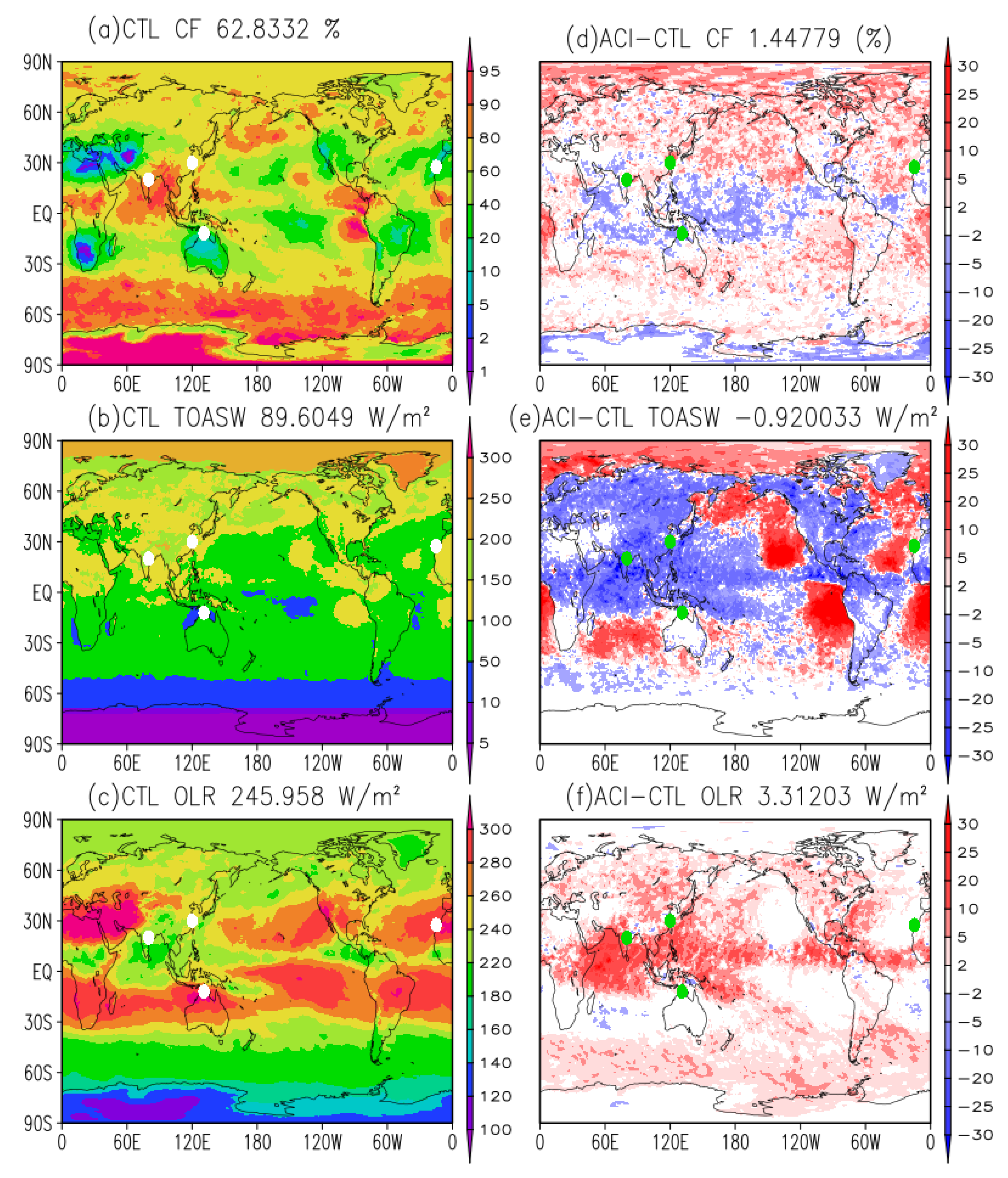
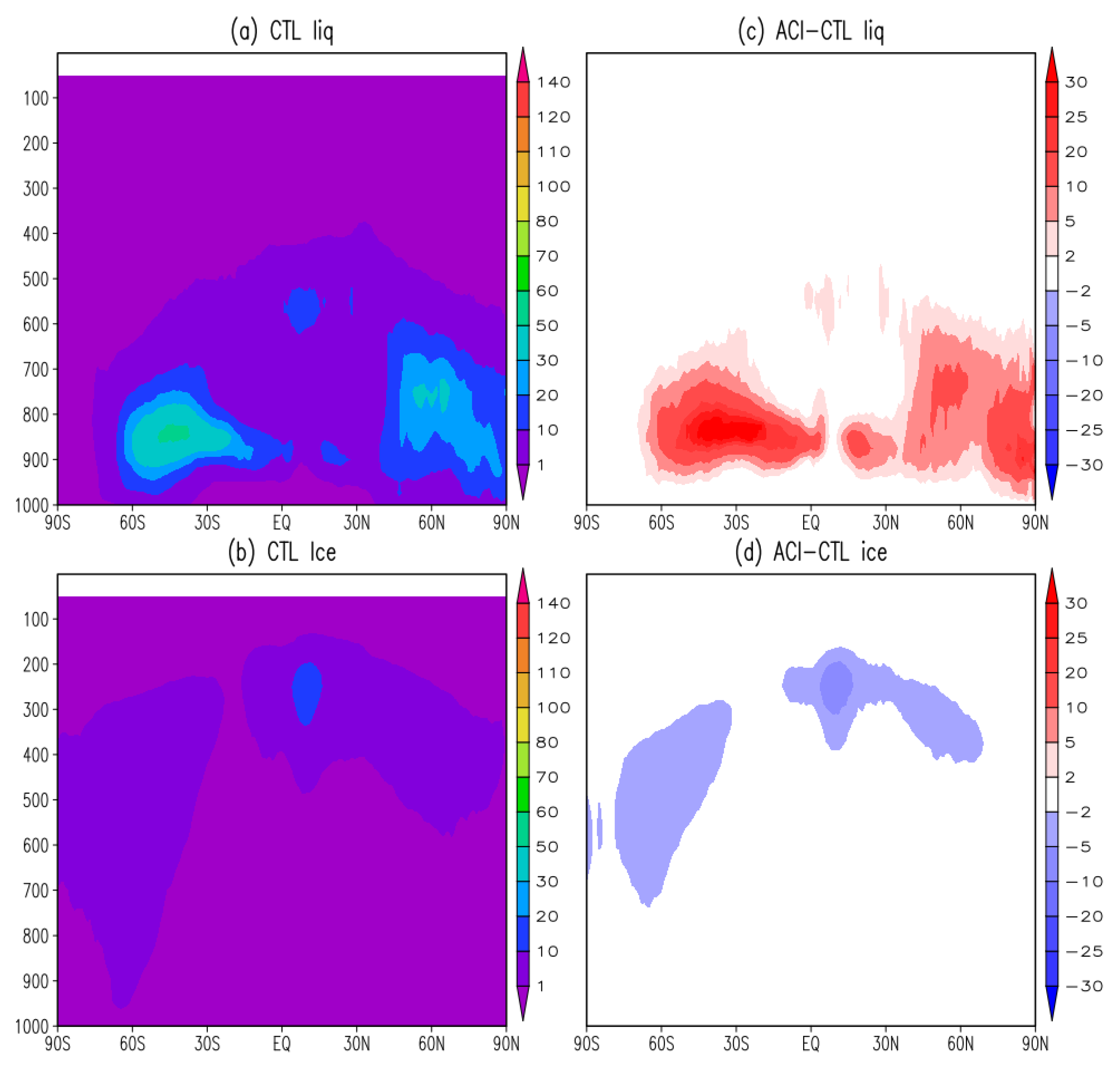
3.1. Global Distribution of Cloud Fractions and Radiation Fluxes

In this section, we examine the aerosol indirect effects by comparing the global distributions of cloud fractions and top-of-atmosphere (TOA) radiation, including longwave (LW) and shortwave (SW) fluxes, between the EXP CTL and EXP ACI. The left three panels of Figure 1 display the global distributions of cloud fraction (a), TOA SW (b), and outgoing longwave radiation (OLR, c) at forecast day 5, averaged for the summer of 2020. Day 5 was selected for analysis as it represents a time with reduced influence from initial conditions while maintaining good forecast skill. For comparison, day 3 exhibits more influence from initial conditions, whereas day 10 demonstrates reduced forecast skill. Nevertheless, results from these days are qualitatively similar. The differences between the EXP CTL and the EXP ACI are shown in the right three panels. The global mean values from the EXP CTL for cloud fraction, TOA SW, and OLR are 62.8%, 89.6 W m⁻², and 246 W m⁻², respectively. The differences between the EXP ACI and CTL are 1.5%, −0.9 W m⁻², and 3.3 W m⁻², respectively. Since positive TOA SW and OLR values represent upward fluxes, the net effect of aerosol–cloud results in a cooling of 2.4 W m⁻².

According to the IPCC Fifth Assessment Report (AR5, [39]), the total Effective Radiative Forcing (ERF) due to aerosols—excluding the effects of absorbing aerosols on snow and ice—ranges from −1.9 to −0.1 W m⁻² with medium confidence. It is important to note that the IPCC’s definition of ERF differs slightly from the net effects of ACI in this study. The IPCC’s ERF primarily focuses on anthropogenic aerosols, such as sulfate, whereas the ACI effects here include contributions from all aerosols, and both experiments use the same MERRA2 climatology to study ACI. Additionally, the EXP CTL predicts and advects ice water number concentrations, and aerosol activation is temperature dependent. As we will show later in the paper, the highly tuned EXP CTL sometimes produces higher ice number concentrations than EXP ACI.

There are good correlations between variations in cloud fraction and TOA radiation fluxes in the EXP ACI relative to the CTL. Increased cloud fractions near the west coasts of North and South America, Africa, and Australia are associated with greater TOA shortwave (SW) radiation reflected and scattered into space in the EXP ACI, resulting in a cooling effect. These regions are predominantly characterized by low-level stratocumulus and shallow cumulus clouds (Figure 1d, [40]. The EXP CTL produces liquid and ice water in clouds, with most liquid water (Figure 2a) and ice water (Figure 2b) located in the Intertropical Convergence Zone (ITCZ) and storm track regions. Additionally, the EXP ACI generates more liquid water in these areas where low clouds dominate (Figure 2c) due to the higher concentration of liquid resulting from water-friendly aerosol activation, as will be discussed later in the paper using results from CCPP-SCM.

In the ITCZ regions and storm track areas of both the northern and southern hemispheres, the EXP ACI shows reduced cloud fractions, leading to greater outgoing longwave radiation (OLR) emitted from these regions (Figure 1f). The clouds in these areas are predominantly deep convective clouds, suggesting that the cloud top temperature in the EXP ACI might be higher, and the cloud tops themselves might be lower. Consistent with this, the ice cloud content in the EXP ACI is significantly lower compared to the EXP CTL (Figure 2d), which can be attributed to the reduced ice number concentration from ice-friendly aerosols.

There are generally positive correlations between low-level cloud fraction and TOA shortwave radiation (SW), and negative correlations between deep cloud fraction and outgoing longwave radiation (OLR). Huang et al. (2019) [41] observed a positive correlation between high-level clouds and TOA SW, and a negative correlation between high-level clouds and OLR using an earlier version of the GFS with a modified single-moment microphysics scheme, incorporating simplified aerosol and radiation interactions. The positive correlation between cloud fraction (whether low- or high-level) and TOA SW is attributed to the reflective and scattering properties of clouds, while the negative correlation between cloud fraction and OLR results from low-level clouds trapping longwave radiation and high-level or deep clouds emitting less longwave radiation.

The relationship between AOD and cloud droplet number concentration (CDNC) is crucial for understanding aerosol–cloud interactions and has been used to reduce uncertainty in numerical models [42]. Since both AOD and CDNC can be observed by satellites and interact directly with aerosols and clouds, they are valuable for both purposes. CDNC is used as an alternative measure to assess the effects of CCN, representing the number of droplets per unit volume at the cloud base. As shown in Figure 3a, AOD and CDNC are strongly correlated in the UFS model, though there is significant variability, as indicated by the large standard deviation. The slope and magnitude of this correlation are comparable to the two global climate models (GCMs) used by Quaas et al. (2005) [42]. Large variability in CDNC highlights uncertainties in factors such as temperature, vertical velocity, aerosol radius, and hygroscopicity during CCN activation.

There are statistically significant positive correlations between AOD and total cloud fraction, likely because clouds form more easily when aerosols act as IN or CCN under conditions of lower moisture. This positive relationship between total cloud fraction and AOD is not only simulated by general circulation models but also observed in satellite data (e.g., [42]). However, the relationship between AOD and TOA radiation fluxes (Figure 3b,c) is more complex. Both TOA SW and outgoing longwave radiation (OLR) show good correlation with AOD when AOD is below 0.1, corresponding to an effective radius of less than 8.2 µm (Figure 3d). These small cloud droplets or ice crystals effectively reflect and scatter shortwave radiation while allowing longwave radiation emitted from the warm surface to pass through. Among these particles, those with an effective radius smaller than 1 µm originate from aerosols in the accumulation mode (a dry radius between 0.1 and 0.5 μm, [43]). These particles exhibit the highest mass extinction efficiency and have the longest atmospheric lifetime ([34]).

When AOD exceeds 0.1, the relationship between AOD and TOA SW and OLR becomes weaker and more uncertain due to additional physical processes like precipitation. In fact, the OLR and AOD even show a negative correlation in some cases, likely because clouds with high AOD can effectively block longwave radiation from the surface (Figure 1f). Notably, the trend of the effective radius is similar to those of TOA SW and OLR, highlighting the significant role of effective radius in determining TOA radiative forcings.

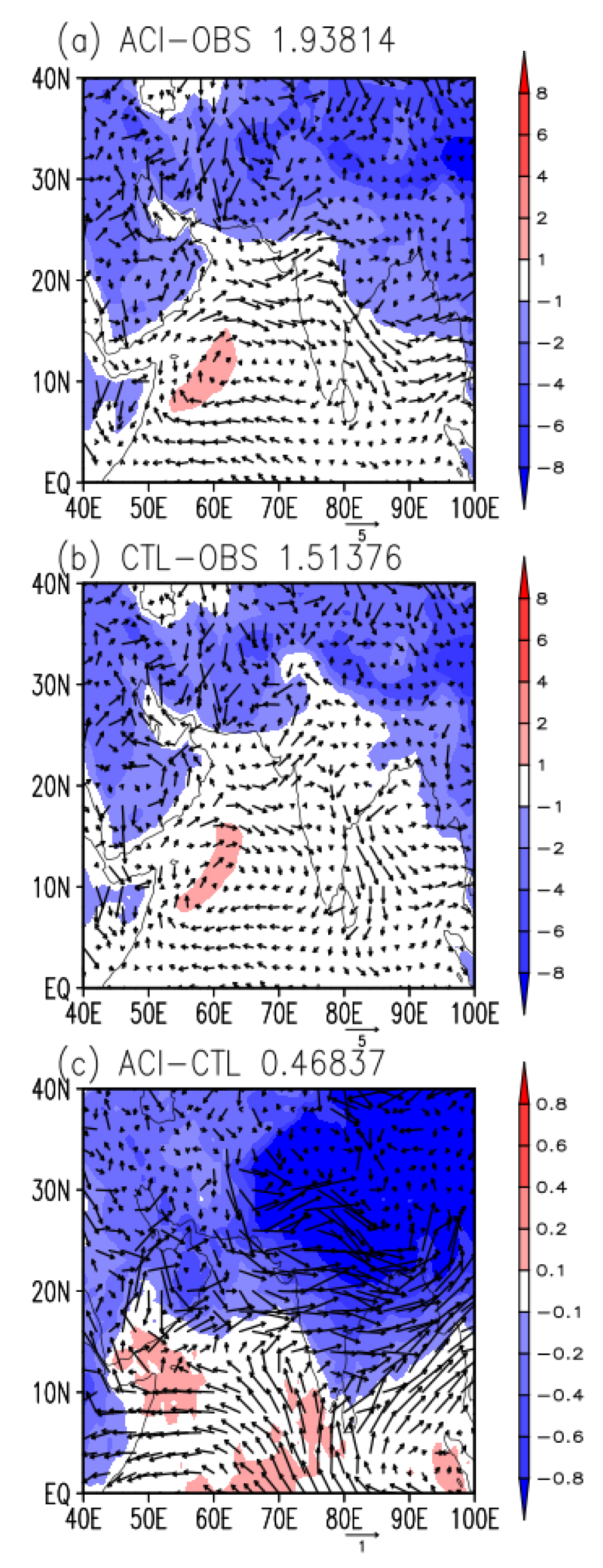
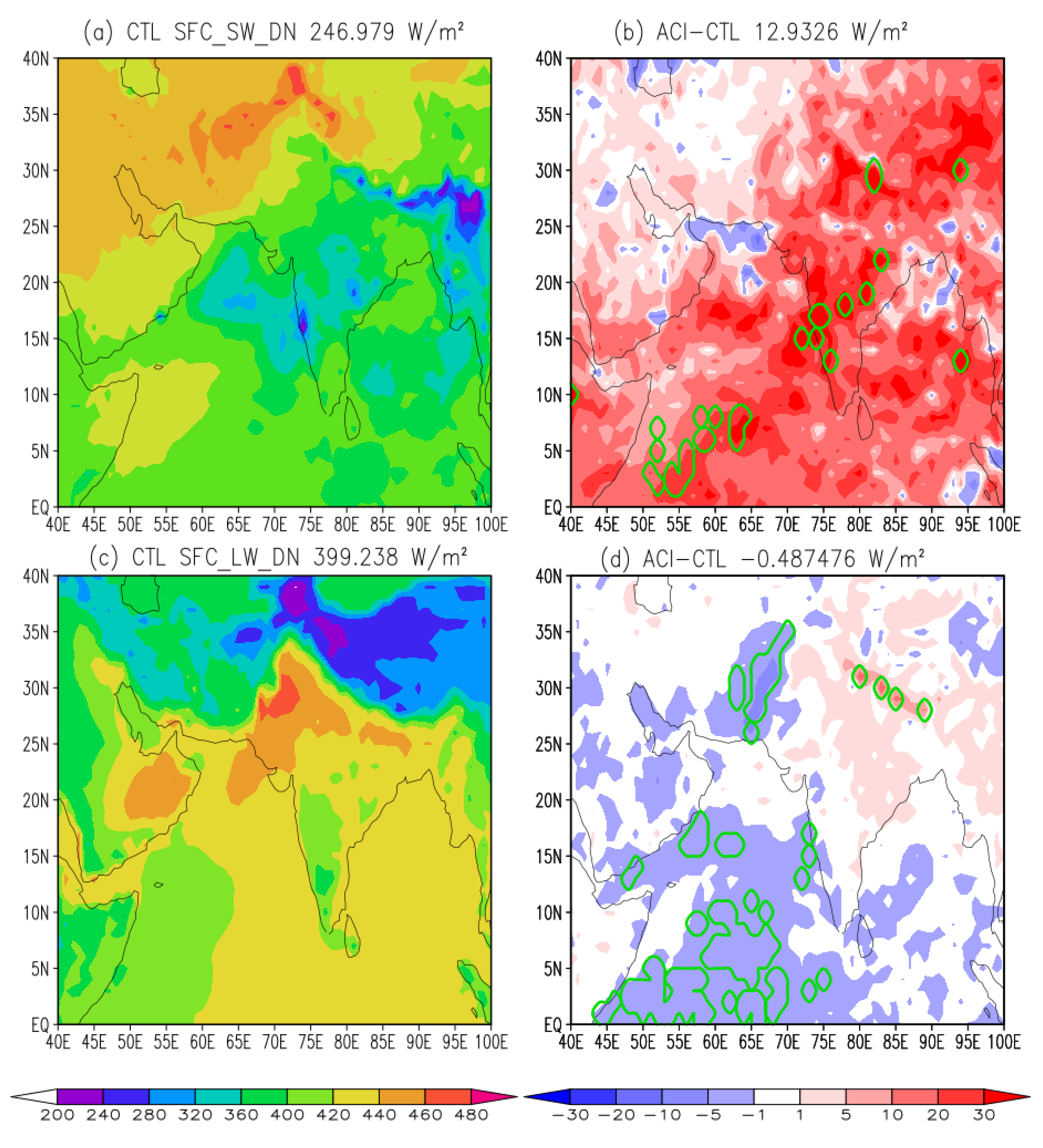
3.2. Impact on India Monsoon

Figure 4a–c display the monsoon circulation, represented by the 850 hPa wind and surface pressure differences for the summer of 2020, EXP ACI subtracting OBS, EXP CTL subtracting OBS, and ACI subtracting CTL, respectively. Both experiments (Figure 4a,b) reveal an anomalous anticyclonic circulation over the Indian Ocean. A southward monsoon flow bias is observed south of 20° N and between 60° E and 90° E in both experiments, though this bias is reduced in the EXP ACI (Figure 4c). The stronger northward flow in the EXP ACI suggests a more robust monsoon circulation compared to the CTL, aligning with findings from Mulcahy et al. (2014) [27]. Both experiments underestimate surface pressure over land while slightly overestimating sea level pressure (SLP) over the ocean.

The regional mean surface latent heat flux (93.6 W m⁻², Figure 5a) is about three times higher than the regional sensible heat flux (36.7 W m⁻², Figure 5c) for EXP CTL. Latent heat fluxes are generally larger over oceans, where moisture is abundant, while sensible heat fluxes are more prominent over land. The differences in both latent and sensible fluxes between the two experiments are consistently positive over land, with the largest values near the southern side of the Tibetan Plateau (Figure 5b,d). In the EXP ACI, both types of fluxes contribute to upward motion, which supports the development of monsoon cloud systems in the region.

To better understand the differences in latent and sensible heat fluxes between the two experiments, surface downward shortwave and longwave radiative fluxes from the EXP CTL, as well as the differences between the EXP ACI and the EXP CTL, are shown in Figure 6. Since clouds scatter, reflect, and block shortwave radiation while emitting longwave radiation, the patterns in Figure 6a,c are similar but with opposite signs. The shortwave radiation difference between the ACI and the CTL is mostly positive over the monsoon region, with a regional mean of about 12.9 W m⁻². Positive anomalies in both shortwave and longwave radiation are found in the Indian Peninsula, and the Tibetan Plateau (Figure 6b,d). These radiative fluxes from the EXP ACI over the monsoon region warm the surface, increasing near-surface temperatures and enhancing surface heating, which leads to higher latent and sensible fluxes.

To investigate what types of clouds contribute to the increased downward longwave and shortwave radiative fluxes, it is important to note that clouds usually block shortwave radiation and emit longwave radiation. A typical point located at 80° E and 20° N in the Indian monsoon region was selected, and the CCPP-SCM was used to simulate the scenario using forcing data derived from GFS outputs. The study site was carefully selected based on its representativeness: a cloud fraction of 80%, TOA upward shortwave radiation of 120 W m⁻², and OLR of 200 Wm⁻² (Figure 1). Surface latent and sensible heat fluxes (Figure 5), as well as surface downward shortwave and longwave radiation (Figure 6), fall within the region of interest. This selection may also explain why the EXP ACI produces more liquid water and low-level clouds (Figure 1d and Figure 2c). The forecasts began on 2020/06/01/00 UTC and ran for ten days. The mean ice water number concentration for the last five days (Figure 7a), ice mixing ratio (Figure 7b), liquid water number concentration (Figure 7c), and liquid water mixing ratio (Figure 7d) are plotted. The EXP CTL produces higher ice water number concentration, more ice, and more high-level clouds. This is expected because GFS has been calibrated to predict current weather conditions, and the temperature-dependent ice number concentration has been tuned to generate reasonable high-level clouds, ensuring outgoing longwave and shortwave radiation matches satellite observations. The other reason is that the EXP CTL uses the same aerosol climatology as the EXP ACI, not like the IPCC control runs that used the pre-industrial aerosols. The EXP ACI, which also uses climatological aerosol data, generates fewer high clouds, allowing more shortwave radiation to pass through. On the other hand, the EXP ACI produces a higher liquid water number concentration compared to the EXP CTL, which uses a fixed value of 10⁸ m⁻³. Consequently, the EXP ACI forms more liquid and low-level clouds. These low-level clouds are warmer and tend to emit more longwave radiation back toward the surface.

3.3. Stratocumulus Clouds

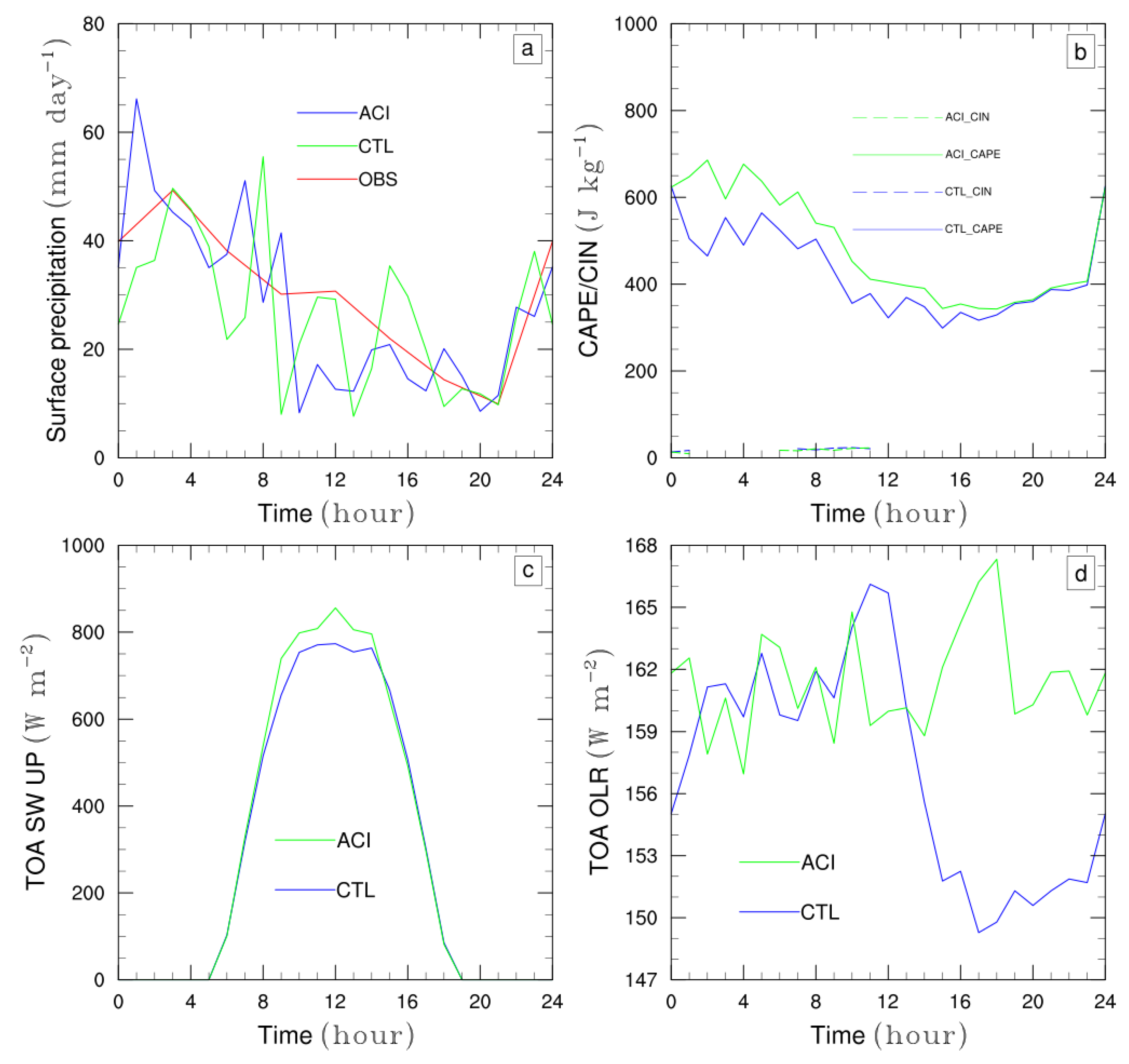
Stratocumulus clouds are typically found along the western coasts of subtropical continents and in the descending branches of large-scale circulations. Although these clouds have a limited impact on outgoing longwave radiation (OLR) due to the minimal temperature difference between the cloud tops and the surface, they significantly contribute to reflecting shortwave radiation. Stratocumulus clouds are influenced not only by large-scale meteorological conditions (e.g., [40,45]) but also by aerosol particles emitted from land and ocean. Generally, an increase in aerosols leads to the formation of smaller but more cloud droplets, which in turn results in larger cloud coverage, increased liquid water path, higher cloud albedo, and reduced precipitation (e.g., [46,47]).

The Atlantic Stratocumulus Transition Experiment (ASTEX) was conducted over the northeast Atlantic Ocean to study stratocumulus clouds and their transition to subtropical trade cumulus regimes using aircraft, ship, and satellite observations [48]. In this study, the CCPP-SCM was used to investigate the aerosol indirect effects for ASTEX. Initial conditions and forcing data were taken from large eddy simulation (LES) intercomparison studies, based on the second (A209) and third flight (RF06) of ASTEX’s first Lagrangian ([49,50]). The SCM was run for 40 h to reach a steady state. Without aerosol effects, the CTL experiment underestimates the liquid water mixing ratio (Figure 8). The EXP ACI, which uses a constant liquid water number concentration as specified by the LES intercomparison study, tends to produce smaller but more cloud droplets than the EXP CTL, where the liquid water mixing ratio depends solely on temperature. The liquid water mixing ratio in the EXP ACI increases and aligns more closely with LES results. To further explore the effects of aerosols, liquid water number concentration was forecasted, and cloud condensation nuclei (CCN) activation was turned on using aerosol data from the MERRA2 climatology. In this case, the liquid water number concentration was no longer constant, reaching its highest values near the surface and decreasing toward zero near the cloud top (Figure 9a, green line). Note that the liquid water number concentration increases due to the air density decreasing, although it is prescribed as 10⁸ m⁻³ for the EXP CTL (Figure 9a, red line and black line are overlapped). Larger liquid water amounts near the surface were produced, as well as a decrease in drizzle, which contributes to liquid water (Figure 9b, green line). This was also observed in other stratocumulus studies (e.g., [51]) and might be another reason that the EXP ACI produces more liquid water and low-level clouds as shown in Figure 1d and Figure 2c.

3.4. Diurnal Cycle

An important aspect of weather systems is the diurnal cycle. Many processes control this cycle, including precipitation, large-scale meteorological conditions, and aerosol–cloud–radiation interactions. While much research has focused on the influence of large-scale forcing and convection on the diurnal cycle of aerosols (e.g., [52,53,54]), fewer studies have examined the impact of aerosols on the diurnal cycle of cloud systems [55]. Using LESs of pristine and polluted stratocumulus clouds, Sandu et al. (2008) [55] found that an increase in droplet concentration caused by aerosols can either increase or decrease liquid water, depending on factors such as cloud top entrainment, drizzle evaporation, and surface latent and sensible heat fluxes. In this study, we selected a more comprehensive cumulus case from the Tropical Warm Pool International Cloud Experiment (TWPICE; [56]).

The TWPICE took place in January–February 2006 in Darwin during the northern Australian monsoon season. A comprehensive dataset was provided to study the structure and evolution of deep tropical convection, shallow cumulus clouds, high-level cirrus clouds, and radiation using a variety of instruments. A major Madden–Julian oscillation (MJO) event influenced the region, and various tropical convective systems originating from the ocean, land, and islands were observed during the TWPICE.

The CCPP-SCM was used to study the diurnal cycle of the TWPICE case. Although tropical precipitation tends to peak in the afternoon over land due to boundary layer destabilization (e.g., [57]), precipitation over islands and oceans peaks around 03 Local Sidereal Time (LST), reflecting the nocturnal life cycle of mesoscale convective systems (Figure 10a). The EXP ACI accurately captures the early morning peak, while the EXP CTL’s peak occurs at 01 LST, two hours earlier. Both experiments underestimate precipitation between 08 LST and 20 LST, but the EXP ACI is closer to observations. Convective precipitation accounts for about three-quarters of the total precipitation, with the rest attributed to large-scale processes. CAPE (convective available potential energy) is closely correlated with precipitation (Figure 10b), peaking at 03 LST and decreasing through 20 LST. The EXP ACI consistently generates higher CAPE than the EXP CTL, which helps explain the higher precipitation in the EXP ACI between 08 LST and 20 LST. Convective inhibition (CIN) is shown in Figure 10b, with values much smaller than the CAPE for both experiments. CIN exhibits some effects during midnight and early morning, but its magnitude is consistently close for the two experiments. Additionally, the EXP ACI produces larger TOA upward shortwave radiation flux between 06 LST and 16 LST, while its outgoing longwave radiation is higher between 13 LST and 02 LST. These two effects contribute to cooling the atmospheric column, which may enhance instability and increase CAPE.

To better understand the effects of aerosols, clouds, and radiation on the diurnal cycle of CAPE and surface precipitation, the diurnal cycle of shortwave, longwave, and total radiative heating rates is shown in Figure 11. Shortwave radiative heating primarily warms the layer between 700 hPa and 100 hPa during the daytime, with the EXP ACI showing a larger magnitude (Figure 11a,b). This heating corresponds to a larger ice number concentration (Figure 12c,d), with peaks in the ice mixing ratio lagging by a few hours (Figure 12a,b). The liquid water number concentration is fixed at 10⁸ m⁻³ for the EXP CTL, so it is not plotted. Shortwave heating stabilizes the atmosphere by warming the upper troposphere, which is one factor contributing to the reduced surface precipitation and CAPE during the day, along with the release of CAPE by early morning convective activity.

Conversely, longwave radiative heating cools the upper troposphere and warms the lower troposphere (Figure 11c,d), helping generate CAPE. The combined effect of radiative heating is that shortwave heating reduces CAPE during the day, while longwave heating increases CAPE starting at 16 LST, with CAPE reaching its maximum in the early morning, initiating strong convective activity. Both shortwave and longwave heating are more intense in the EXP ACI, likely due to the higher aerosol concentration, which results in smaller but more ice crystals. These ice crystals absorb shortwave radiation, warming the atmosphere, and emit longwave radiation, cooling it.

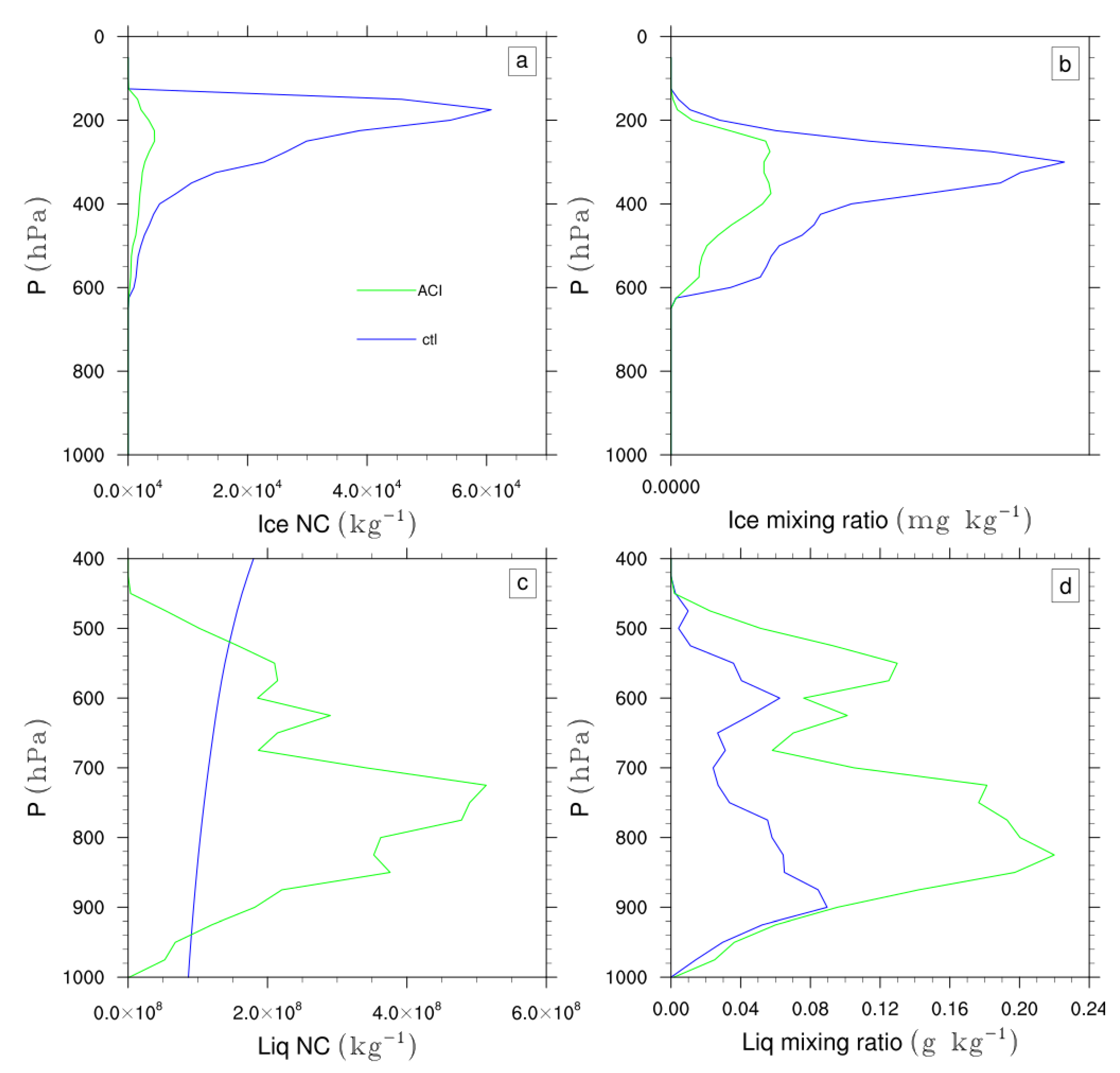
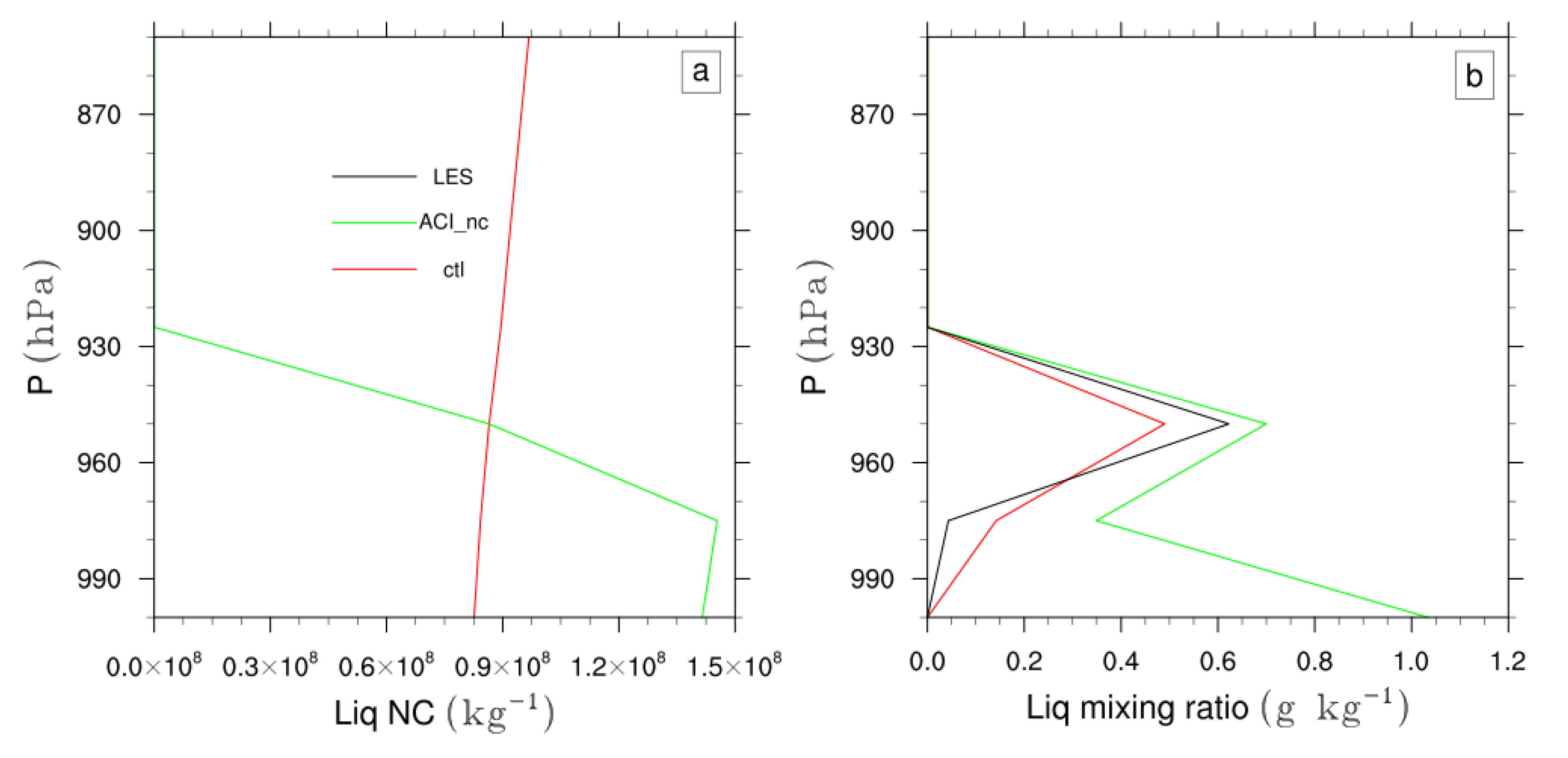
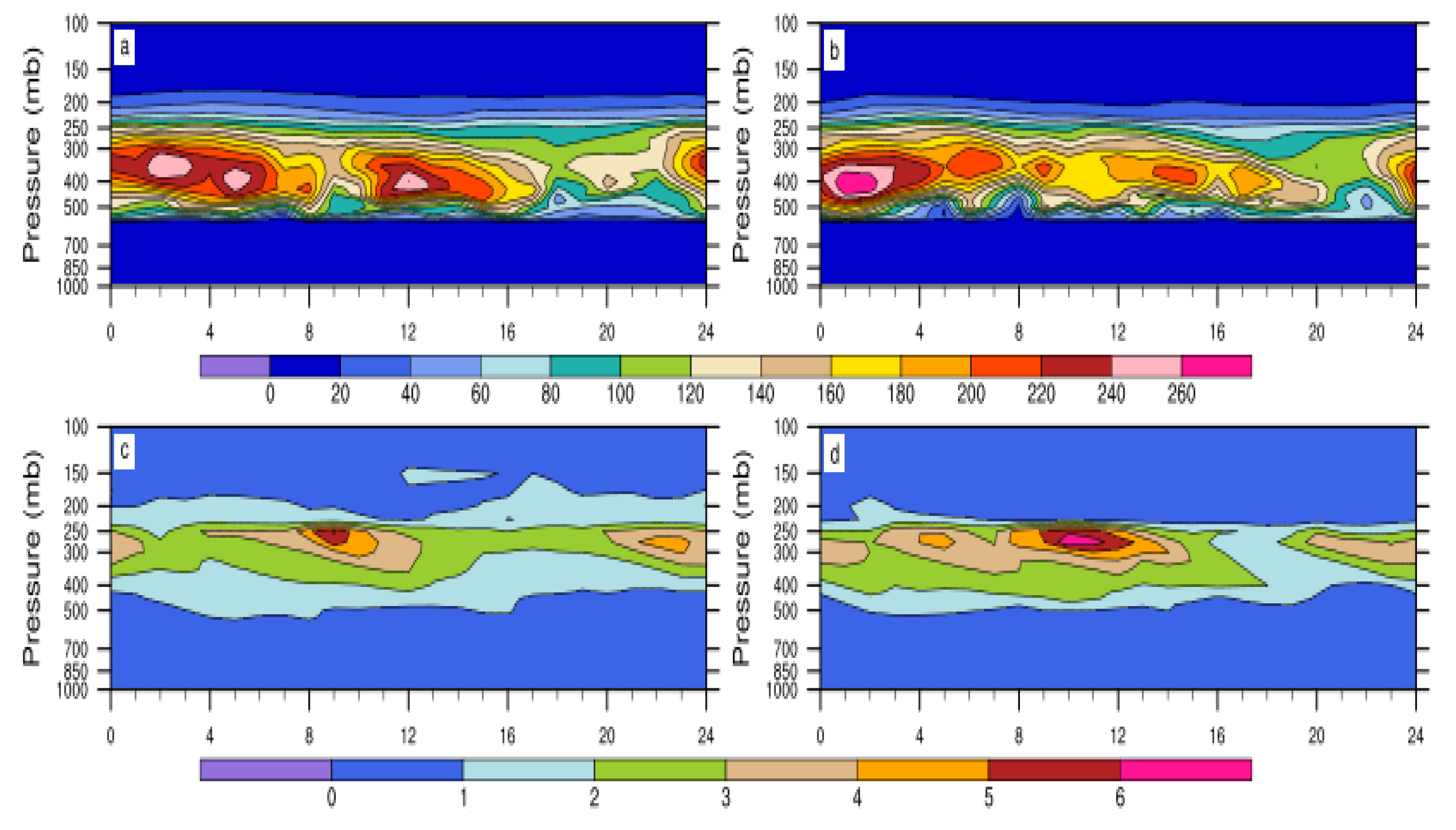
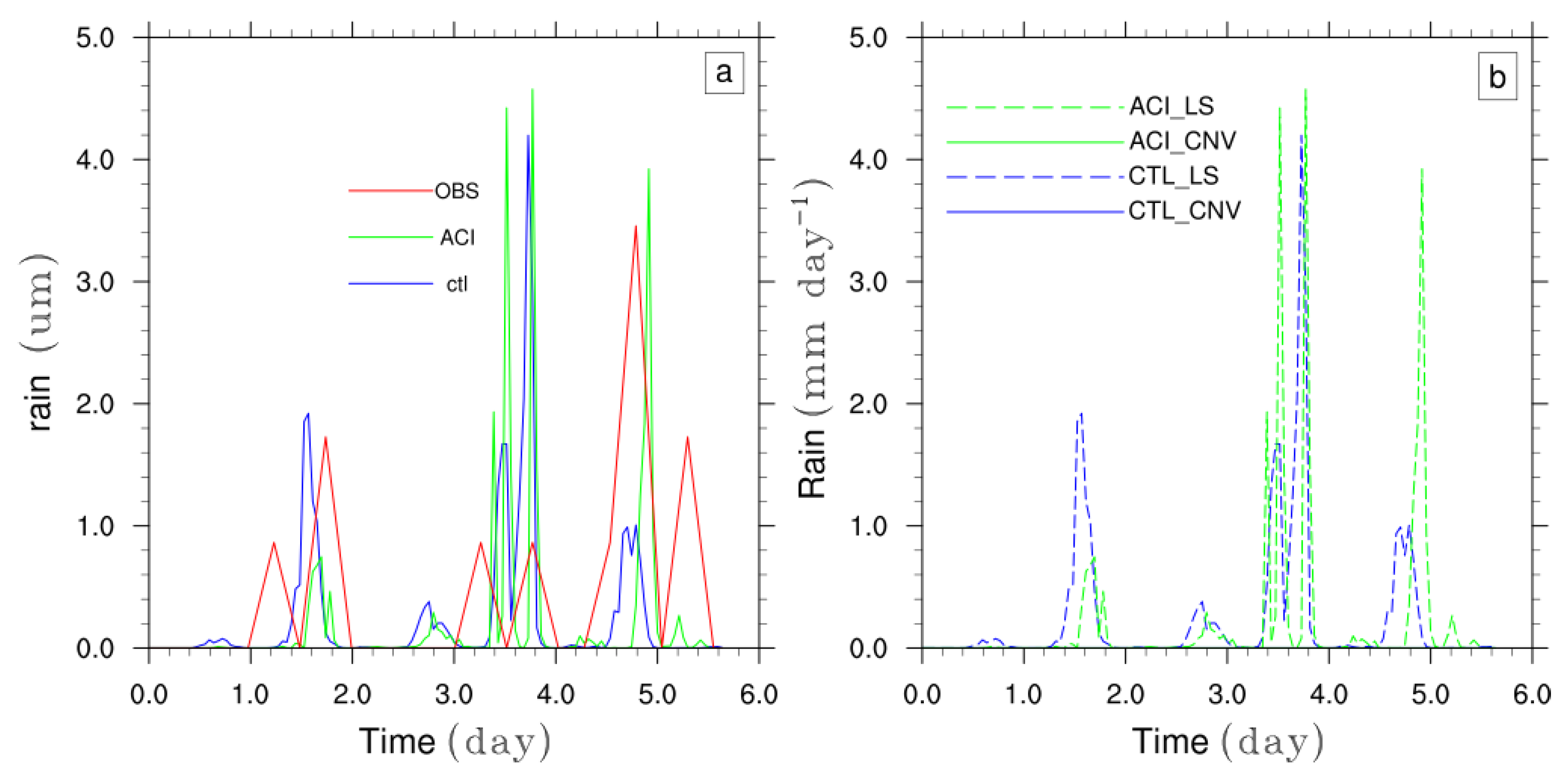
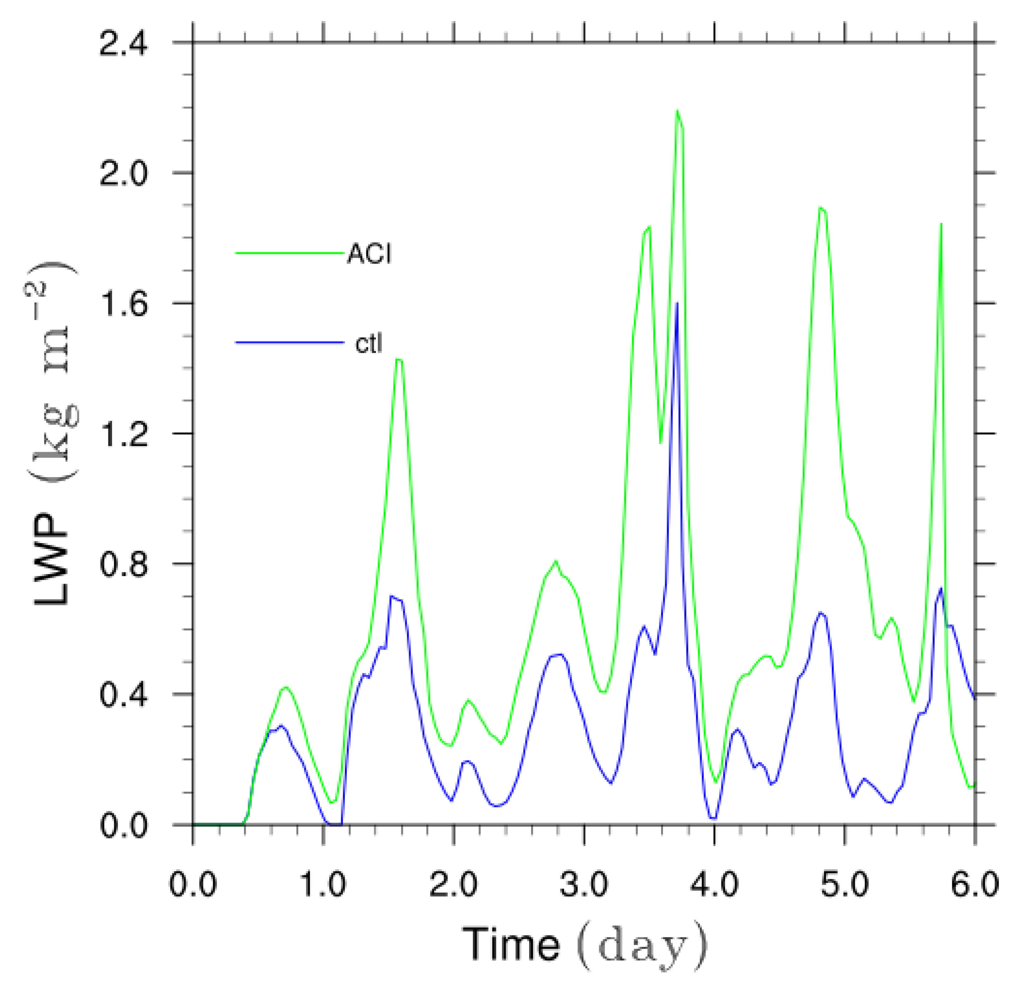
3.5. Deep Convection Invigoration and Cloud System Life Cycle

A deep convective system located in the warm pool at 15° N and 120° E, starting on 1 June 2020, at 00 UTC, was chosen to study the effects of aerosols on deep convection invigoration. The study location was chosen for its proximity to Asia, which exposes it to continental aerosol influences, and its closeness to the warm pool, minimizing horizontal advection effects. The environmental relative humidity is around 70%, and the vertical wind shear is weak. Horizontal advection of moisture and temperature is minimal, making the system relatively stationary. To confirm this, an SCM run was performed without horizontal advection, yielding results similar to those with horizontal advection.

There are several precipitation episodes during the 6 h free forecasts (Figure 13a). The results indicate that large-scale precipitation dominates during the six-hour forecasts, with aerosol impacts seen in the delayed precipitation in the EXP ACI, due to smaller but more numerous liquid and ice particles. The last two precipitation episodes may be related to aerosol invigoration in the EXP ACI. While there is no clear evidence of an increased precipitation life cycle, the liquid water path (LWP, Figure 14) suggests a longer cloud system life span. The increased LWP could have a significant impact on radiation fluxes, making it important for the energy budget of climate systems.

To further investigate aerosol invigoration effects on precipitation cloud systems, we analyzed the liquid water number concentration and mixing ratio, averaged between hours 4 and 5.5 (Figure 15a,b). The experimental period was selected for two reasons: (1) aerosol loading in the EXP ACI resulted in prolonged events (Figure 14), and (2) aerosol invigoration suppressed warm-cloud precipitation, enhancing supercooled water transport to higher altitudes, which formed ice clouds, as shown in the EXP ACI (shown later). In the EXP ACI, both the liquid water number concentration and mixing ratio are significantly larger, with distinct peaks at 850 hPa and 600 hPa. The cloud top in the EXP ACI is also slightly higher than in the EXP CTL. Additionally, ice clouds are present near 250 hPa in the EXP ACI (Figure 16a,b), whereas no ice clouds are observed in the EXP CTL. These ice clouds may release more latent heat, indicating a stronger cloud system in the EXP ACI.

The microphysical heating rates for both experiments are shown in Figure 17. While the heating rate in the EXP ACI is smaller below 500 hPa, it is larger above this level. The clouds at 600 hPa in the EXP ACI are in a mixed phase, and the heating rates in this region could suppress warm cloud precipitation, enhancing supercooled water that is transported upward to form ice clouds, as shown in Figure 16. This process is another mechanism of aerosol invigoration, as reported by Khain (2009) [16] and Altaratz et al. (2014) [15].

4. Discussion and Conclusions

In this study, interactions between aerosols, clouds, and radiation in the GFS.V17.p8 are evaluated. Two experiments were conducted for the summer of 2020. In the control experiment (EXP CTL), aerosols are coupled only with radiation, including direct and semi-direct aerosol effects. In the sensitivity experiment (EXP ACI), aerosols are coupled with both radiation and Thompson microphysics, allowing for full interaction between aerosols and clouds, including indirect aerosol effects. MERRA2 climatological aerosols are used to diagnose NIFA and NWFA, which activate ice nuclei (IN) and cloud condensation nuclei (CCN). Introducing aerosol–cloud interactions results in a net cooling of 2.4 W/m² at the top of the atmosphere (TOA). Further analysis reveals that the EXP ACI produces more liquid water at lower levels and less ice water at higher levels compared to the EXP CTL, with TOA cooling driven by increased outgoing longwave radiation (OLR) from low-level clouds. AOD (Aerosol Optical Depth) shows a strong linear relationship with cloud droplet number concentration (CDNC), similar to other climate models, though with large standard deviations. However, AOD correlates well with effective radius, TOA shortwave radiation, and OLR only when AOD is below 0.1, possibly due to the complexity introduced by additional processes such as precipitation and collision–coalescence when AOD is larger than 0.1.

The impact of aerosol–cloud interactions on the Indian Summer Monsoon was also examined. In the EXP ACI, fewer high clouds are produced, and they tend to form at lower altitudes compared to the highly tuned control experiment (EXP CTL). This results in greater transparency to shortwave radiation and increased downward shortwave flux at the surface. However, the liquid water number concentration is generally higher in the EXP ACI, leading to the formation of more liquid and low-level clouds. These low-level liquid water clouds are relatively warm, emitting more longwave radiation back to the surface. The combination of increased downward shortwave and longwave fluxes contributes to surface warming and moistening, especially given the high moisture levels in the Indian monsoon region. As a result, surface sensible and latent heat fluxes increase over the land, driving a northward flow south of 20° N between 60° E and 90° E in the EXP ACI. This reduces the southward bias and suggests a stronger Indian Summer Monsoon.

In a stratocumulus case study (ASTEX), the liquid water mixing ratio increases in the EXP ACI due to the formation of smaller cloud droplets from the higher aerosol concentration. This result aligns more closely with those from large eddy simulations (LES). Additionally, cloud-base evaporation from drizzle enhances near-surface liquid water in this case.

The TWPICE was selected to study the influence of aerosols on diurnal cycles. In the control experiment (EXP CTL), the peak precipitation occurs two hours earlier than observed, while the EXP ACI captures the timing of the peak more accurately. This improvement is likely to be due to the presence of smaller but more numerous cloud droplets and ice crystals in the EXP ACI, which delays the peak precipitation. Another notable difference between the two experiments is that the EXP CTL underestimates late afternoon precipitation more significantly. Further analysis shows that CAPE (Convective Available Potential Energy) correlates well with precipitation in both experiments. The shortwave and longwave heating are stronger in the EXP ACI due to the higher aerosol concentrations, which produce smaller but more abundant ice crystals. These ice crystals may absorb shortwave radiation, warming the lower to middle troposphere, while emitting longwave radiation that cools the upper troposphere, contributing to greater CAPE. Notably, aerosol concentrations are higher in the EXP ACI compared to the Indian monsoon case.

The effects of aerosols on deep convection and cloud system lifespan were also analyzed in a warm pool region case. In this humid environment, characterized by weak vertical wind shear and minimal horizontal advection of moisture and temperature, warm rain processes may be suppressed by heating in mixed-phase clouds. This, in turn, enhances supercooled water, which is transported upward to form more ice clouds. While no direct evidence of an extended precipitation life cycle was found, the EXP ACI produced more precipitation, and an increase in cloud system lifespan was observed in the liquid water path.

References

1. Haywood, J.; Boucher, O. Estimates of the direct and indirect radiative forcing due to tropospheric aerosols: A review. Rev. Geophys. 2000, 38, 513–543. [Google Scholar] [CrossRef]
2. Myhre, G. Consistency Between Satellite-Derived and Modeled Estimates of the Direct Aerosol Effect. Science 2009, 325, 187–190. [Google Scholar] [CrossRef] [PubMed]
3. Koch, D.; Del Genio, A.D. Black carbon absorption effects on cloud cover: Review and synthesis. Atmos. Chem. Phys. 2010, 10, 7685–7696. [Google Scholar] [CrossRef]
4. Twomey, S. The influence of pollution on the shortwave albedo of clouds. J. Atmos. Sci. 1977, 34, 1149–1152. [Google Scholar] [CrossRef]
5. Penner, J.E.; Andreae, M.; Annegarn, H.; Barrie, L.; Feichter, J.; Hegg, D.; Jayaraman Leaitch, R.; Murphy, D.; Nganga, J.; Pitari, G. Aerosols, Their Direct and Indirect Effects7, in Climate Change 2001: The Scientific Basis, Contribution of Working Group I to the Third Assessment Report of the Intergovernmental Panel on Climate Change; Houghton, J.T., Ding, Y., Griggs, D.J., Noguer, M., Van der Linden, P.J., Dai, X., Maskell, K., Johnson, C.A., Eds.; Cambridge University Press: New York, NY, USA, 2001; p. 881. [Google Scholar]
6. Fan, J.; Yuan, T.; Comstock, J.M.; Ghan, S.; Khain, A.; Leung, L.R.; Li, Z.; Martins, V.J.; Ovchinnikov, M. Dominant role by vertical wind shear in regulating aerosol effects on deep convective clouds. J. Geophys. Res. Atmos. 2009, 114, D22206. [Google Scholar] [CrossRef]
7. Fan, J.; Wang, Y.; Rosenfeld, D.; Liu, X. Review of aerosol–cloud interactions: Mechanisms, significance, and challenges. J. Atmos. Sci. 2016, 73, 4221–4252. [Google Scholar] [CrossRef]
8. Khain, A.; Rosenfeld, D.; Pokrovsky, A. Aerosol impact on the dynamics and microphysics of deep convective clouds. Q. J. R. Meteorol. Soc. 2005, 131, 2639–2663. [Google Scholar] [CrossRef]
9. Li, Z.; Niu, F.; Fan, J.; Liu, Y.; Rosenfeld, D.; Ding, Y. Long-term impacts of aerosols on the vertical development of clouds and precipitation. Nat. Geosci. 2011, 4, 888–894. [Google Scholar] [CrossRef]
10. Hoeve, J.E.T.; Jacobson, M.Z.; Remer, L.A. Comparing results from a physical model with satellite and in situ observations to determine whether biomass burning aerosols over the Amazon brighten or burn off clouds. J. Geophys. Res. Atmos. 2012, 117, D08203. [Google Scholar] [CrossRef]
11. Heever, S.C.V.D.; Carrió, G.G.; Cotton, W.R.; DeMott, P.J.; Prenni, A.J. Impacts of Nucleating Aerosol on Florida Storms. Part I: Mesoscale Simulations. J. Atmos. Sci. 2006, 63, 1752–1775. [Google Scholar] [CrossRef]
12. Devasthale, A.; Kruger, O.; Grassl, H. Change in Cloud-Top Temperatures Over Europe. IEEE Geosci. Remote Sens. Lett. 2005, 2, 333–336. [Google Scholar] [CrossRef]
13. Jiang, H.; Feingold, G. Effect of aerosol on warm convective clouds: Aerosol-cloud-surface flux feedbacks in a new coupled large eddy model. J. Geophys. Res. Atmos. 2006, 111, D1. [Google Scholar] [CrossRef]
14. Xue, H.; Feingold, G.; Stevens, B. Aerosol Effects on Clouds, Precipitation, and the Organization of Shallow Cumulus Convection. J. Atmos. Sci. 2008, 65, 392–406. [Google Scholar] [CrossRef]
15. Altaratz, O.; Koren, I.; Remer, L.; Hirsch, E. Review: Cloud invigoration by aerosols—Coupling between microphysics and dynamics. Atmos. Res. 2014, 140–141, 38–60. [Google Scholar] [CrossRef]
16. Khain, A.P. Notes on state-of-the-art investigations of aerosol effects on precipitation: A critical review. Environ. Res. Lett. 2009, 4, 015004. [Google Scholar] [CrossRef]
17. Morrison, H.; Grabowski, W.W. Response of Tropical Deep Convection to Localized Heating Perturbations: Implications for Aerosol-Induced Convective Invigoration. J. Atmos. Sci. 2013, 70, 3533–3555. [Google Scholar] [CrossRef]
18. Guo, L.; Turner, A.G.; Highwood, E.J. Local and Remote Impacts of Aerosol Species on Indian Summer Monsoon Rainfall in a GCM. J. Clim. 2016, 29, 6937–6955. [Google Scholar] [CrossRef]
19. Lau, K.-M.; Ramanathan, V.; Wu, G.-X.; Li, Z.; Tsay, S.C.; Hsu, C.; Sikka, R.; Holben, B.; Lu, D.; Tartari, G.; et al. The Joint Aerosol–Monsoon Experiment: A New Challenge for Monsoon Climate Research. Bull. Am. Meteorol. Soc. 2008, 89, 369–384. [Google Scholar] [CrossRef]
20. Ramanathan, V.; Crutzen, P.J.; Lelieveld, J.; Mitra, A.P.; Althausen, D.; Anderson, J.; Andreae, M.O.; Cantrell, W.; Cass, G.R.; Chung, C.E.; et al. Indian Ocean Experiment: An integrated analysis of the climate forcing and effects of the great Indo-Asian haze. J. Geophys. Res. Atmos. 2001, 106, 28371–28398. [Google Scholar] [CrossRef]
21. Bollasina, M.A.; Ming, Y.; Ramaswamy, V. Anthropogenic Aerosols and the Weakening of the South Asian Summer Monsoon. Science 2011, 334, 502–505. [Google Scholar] [CrossRef]
22. Ackerman, A.S.; Toon, O.B.; Stevens, D.E.; Heymsfield, A.J.; Ramanathan, V.; Welton, E.J. Reduction of Tropical Cloudiness by Soot. Science 2000, 288, 1042–1047. [Google Scholar] [CrossRef] [PubMed]
23. Chung, C.E.; Ramanathan, V.; Kiehl, J.T. Effects of the South Asian Absorbing Haze on the Northeast Monsoon and Surface–Air Heat Exchange. J. Clim. 2002, 15, 2462–2476. [Google Scholar] [CrossRef]
24. Bozzo, A.; Remy, S.; Benedetti, A.; Flemming, J.; Bechtold, P.; Rodwell, M.J.; Morcrette, J.-J. Implementation of a CAMS-Based Aerosol Climatology in the IFS; ECMWF Technical Memoranda; ECMWF: Reading, UK, 2017; Volume 801, 33p. [Google Scholar]
25. Cheng, A.; Yang, F. Direct radiative effects of aerosols on numerical weather forecast—A comparison of two aerosol datasets in the NCEP GFS. Weather Forecast. 2023, 38, 753–772. [Google Scholar] [CrossRef]
26. Zhang, L.; Montuoro, R.; McKeen, S.A.; Baker, B.; Bhattacharjee, P.S.; Grell, G.A.; Henderson, J.; Pan, L.; Frost, G.J.; McQueen, J.; et al. Development and evaluation of the Aerosol Forecast Member in the National Center for Environment Prediction (NCEP)’s Global Ensemble Forecast System (GEFS-Aerosols v1). Geosci. Model Dev. 2022, 15, 5337–5369. [Google Scholar] [CrossRef]
27. Mulcahy, J.P.; Walters, D.N.; Bellouin, N.; Milton, S.F. Impacts of increasing the aerosol complexity in the Met Office global numerical weather prediction model. Atmos. Chem. Phys. 2014, 14, 4749–4778. [Google Scholar] [CrossRef]
28. Yang, F.; Tallapragada, V.; Kain, J.; Wei, H.; Yang, R.; Yudin, A.V.; Moorthi, S.; Han, J.; Hou, Y.-T.; Wang, J.; et al. Model Upgrade Plan and Initial Results from a Prototype NCEP Global Forecast System Version 16. In Proceedings of the 10th Conference on Transition of Research to Operations, 100th AMS Annual Meeting, Boston, MA, USA, 12–16 January 2020; Available online: https://ams.confex.com/ams/2020Annual/meetingapp.cgi/Paper/362797 (accessed on 1 February 2020).
29. Thompson, G.; Field, P.R.; Rasmussen, R.M.; Hall, W.D. Explicit Forecasts of Winter Precipitation Using an Improved Bulk Microphysics Scheme. Part II: Implementation of a New Snow Parameterization. Mon. Weather Rev. 2008, 136, 5095–5115. [Google Scholar] [CrossRef]
30. Thompson, G.; Rasmussen, R.M.; Manning, K.W. Explicit forecasts of winter precipitation using an improved bulk microphysics scheme. Part I: Description and sensitivity analysis. Mon. Wea. Rev. 2004, 132, 519–542. [Google Scholar] [CrossRef]
31. Mlawer, E.J.; Taubman, S.J.; Brown, P.D.; Iacono, M.J.; Clough, S.A. Radiative transfer for inhomogeneous atmospheres: RRTM, a validated correlated-k model for the longwave. J. Geophys. Res. 1997, 102, 16663–16682. [Google Scholar] [CrossRef]
32. Mlawer, E.J.; Clough, S.A. Shortwave and longwave enhancements in the rapid radiative transfer model. In Proceedings of the Seventh Atmospheric Radiation Measurement (ARM) Science Team Meeting, San Antonio, TX, USA, 3–7 March 1997; United States Department of Energy: Washington, DC, USA, 1998; pp. 409–413. [Google Scholar]
33. Mlawer, E.J.; Iacono, M.J.; Pincus, R.; Barker, H.W.; Oreopoulos, L.; Mitchell, D.L. Contributions of the ARM Program to Radiative Transfer Modeling for Climate and Weather Applications. Meteorol. Monogr. 2016, 57, 15.1-15.19. [Google Scholar] [CrossRef]
34. Buchard, V.; Randles, C.A.; da Silva, A.M.; Darmenov, A.; Colarco, P.R.; Govindaraju, R.; Ferrare, R.; Hair, J.; Beyersdorf, A.J.; Ziemba, L.D.; et al. The MERRA-2 Aerosol Reanalysis, 1980-Onward, Part II: Evaluation and Case Studies. J. Clim. 2017, 30, 6851–6872. [Google Scholar] [CrossRef]
35. Randles, C.A.; Da Silva, A.M.; Buchard, V.; Colarco, P.R.; Darmenov, A.; Govindaraju, R.; Smirnov, A.; Holben, B.; Ferrare, R.; Hair, J.; et al. The MERRA-2 Aerosol Reanalysis, 1980 Onward. Part I: System Description and Data Assimilation Evaluation. J. Clim. 2017, 30, 6823–6850. [Google Scholar] [CrossRef] [PubMed]
36. DeMott, P.J.; Prenni, A.J.; Rogers, D.C. Predicting global atmospheric ice nuclei distributions and their impacts on climate. Proc. Natl. Acad. Sci. USA 2010, 107, 11217–11222. [Google Scholar] [CrossRef] [PubMed]
37. Feingold, G.; Heymsfield, A.J. Parameterizations of Condensational Growth of Droplets for Use in General Circulation Models. J. Atmos. Sci. 1992, 49, 2325–2342. [Google Scholar] [CrossRef]
38. Cooper, W.A. Ice Initiation in Natural Clouds. Meteorol. Monogr. 1986, 43, 29–32. [Google Scholar] [CrossRef]
39. Boucher, O.; Randall, D.; Artaxo, P.; Bretherton, C.; Feingold, G.; Forster, P.; Kerminen, V.-M.; Kondo, Y.; Liao, H.; Lohmann, U.; et al. Clouds and Aerosols. In Climate Change 2013: The Physical Science Basis. Contribution of Working Group I to the Fifth Assessment Report of the Intergovernmental Panel on Climate Change; Stocker, T.F., Qin, D., Plattner, G.-K., Tignor, M., Allen, S.K., Boschung, J., Nauels, A., Xia, Y., Bex, V., Midgley, P.M., Eds.; Cambridge University Press: Cambridge, UK; New York, NY, USA, 2013. [Google Scholar]
40. Wood, R. Stratocumulus clouds. Mon. Weather Rev. 2012, 140, 2373–2423. [Google Scholar] [CrossRef]
41. Huang, H.; Gu, Y.; Xue, Y.; Jiang, J.; Zhao, B. Assessing aerosol indirect effect on clouds and regional climate of East/South Asia and West Africa using NCEP GFS. Clim. Dyn. 2019, 52, 5759–5774. [Google Scholar] [CrossRef]
42. Quaas, J.; Boucher, O. Constraining the first aerosol indirect radiative forcing in the LMDZ GCM using POLDER and MODIS satellite data. Geophys. Res. Lett. 2005, 32, L17814. [Google Scholar] [CrossRef]
43. Schwartz, S.E. The whitehouse effect—Shortwave radiative forcing of climate by anthropogenic aerosols: An overview. J. Aerosol. Sci. 1996, 27, 359–382. [Google Scholar] [CrossRef]
44. Kanamitsu, M.; Ebisuzaki, W.; Woollen, J.; Yang, S.-K.; Hnilo, J.J.; Fiorino, M.; Potter, G.L. NCEP-DOE AMIP-II Reanalysis (R-2). Bull. Am. Meteor. Soc. 2002, 83, 1631–1643. [Google Scholar] [CrossRef]
45. Klein, S.A.; Hartmann, D.L. The Seasonal Cycle of Low Stratiform Clouds. J. Clim. 1993, 6, 1587–1606. [Google Scholar] [CrossRef]
46. Albrecht, B.A. Aerosols, Cloud Microphysics, and Fractional Cloudiness. Science 1989, 245, 1227–1230. [Google Scholar] [CrossRef] [PubMed]
47. Zuidema, P.; Westwater, E.R.; Fairall, C.; Hazen, D. Ship-based liquid water path estimates in marine stratocumulus. J. Geophys. Res. Atmos. 2005, 110, D20206. [Google Scholar] [CrossRef]
48. Albrecht, B.A.; Bretherton, C.S.; Johnson, D.; Scubert, W.H.; Frisch, A.S. The Atlantic Stratocumulus Transition Experiment—ASTEX. Bull. Am. Meteor. Soc. 1995, 76, 889–904. [Google Scholar] [CrossRef]
49. Chlond, A.; Wolkau, A. Large-Eddy Simulation of a Nocturnal Stratocumulus-Topped Marine Atmospheric Boundary Layer: An Uncertainty Analysis. Bound. Layer Meteorol. 2000, 95, 31–55. [Google Scholar] [CrossRef]
50. Duynkerke, P.G.; Jonker, P.J.; Chlond, A.; Van Zanten, M.C.; Cuxart, J.; Clark, P.; Sanchez, E.; Martin, G.; Lenderink, G.; Teixeira, J. Intercomparison of Three- and one-Dimensional Model Simulations and Aircraft Observations of Stratocumulus. Bound. Layer Meteorol. 1999, 92, 453–487. [Google Scholar] [CrossRef]
51. Wood, R. Drizzle in stratiform boundary layer clouds. Part I: Vertical and horizontal structure. J. Atmos. Sci. 2005, 62, 3011–3033. [Google Scholar] [CrossRef]
52. Painemal, D.; Xu, K.-M.; Cheng, A.; Minnis, P.; Palikonda, R. Mean Structure and Diurnal Cycle of Southeast Atlantic Boundary Layer Clouds: Insights from Satellite Observations and Multiscale Modeling Framework Simulations. J. Clim. 2015, 28, 324–341. [Google Scholar] [CrossRef]
53. Stevens, B.; Graham, F. Untangling aerosol effects on clouds and precipitation in a buffered system. Nature 2009, 461, 1476–4687. [Google Scholar] [CrossRef]
54. Xie, S.; Hume, T.; Jakob, C.; Klein, S.; McCoy, R.; Zhang, M. Observed large-scale conditions and diabatic heating and drying profiles during TWP-ICE. J. Clim. 2010, 23, 57–79. [Google Scholar] [CrossRef]
55. Sandu, I.; Brenguier, J.-L.; Geoffroy, O.; Thouron, O.; Masson, V. Aerosol Impacts on the Diurnal Cycle of Marine Stratocumulus. J. Atmos. Sci. 2008, 65, 2705–2718. [Google Scholar] [CrossRef]
56. May, P.T.; Mather, J.H.; Vaughan, G.; Jakob, C.; McFarquhar, G.M.; Bower, K.N.; Mace, G.G. The Tropical Warm Pool International Cloud Experiment. Bull. Am. Meteorol. Soc. 2008, 89, 629–646. [Google Scholar] [CrossRef]
57. Nesbitt, S.W.; Zipser, E.J. The diurnal cycle of rainfall and convective intensity according to three years of TRMM measurements. J. Clim. 2003, 16, 1456–1475. [Google Scholar] [CrossRef]
58. Thompson, G.; Eidhammer, T. A Study of Aerosol Impacts on Clouds and Precipitation Development in a Large Winter Cyclone. J. Atmos. Sci. 2014, 71, 3636–3658. [Google Scholar] [CrossRef]
Figure 1. Global distributions of cloud fraction (a), top-of-atmosphere shortwave radiation (TOA SW) (b), and outgoing longwave radiation (OLR, c) at forecast day 5, averaged over the summer of 2020 from the EXP CTL. Panels (df) show the differences between ACI and CTL. The solid white circles in the left panels and the green solid circles on the right indicate the sites selected for the CCPP-SCM simulations. These sites are located in the Indian monsoon region, ASTEX, TWICE, and the Pacific warm pool.
Meteorology 04 00014 g001
Figure 2. Zonal cross sections of cloud liquid water (a, mg kg−1, rain not included) and cloud ice (b, mg kg−1, snow and graupel not included) on day 5 of the forecasts, averaged over the summer of 2020. Panels (c,d) show the differences between the ACI and CTL experiments.
Meteorology 04 00014 g002
Figure 3. Relationships between aerosol optical depth (AOD) and cloud droplet number concentration (CDNC, a), between AOD and TOA SW (b), between AOD and OLR (c), and between effective radius and OLR (d) for EXP ACI.
Meteorology 04 00014 g003
Figure 4. Distributions of sea level pressure differences (SLP, hPa, shaded), overlaid with 850 hPa vector wind differences (m s−1), between the EXP ACI on day 5 of the forecast, averaged for the summer of 2020, and the NCEP reanalysis (OBS, [44]) over the Asian monsoon region in (a); differences between the EXP CTL and the NCEP reanalysis in (b); and differences between the EXP ACI and the CTL in (c). The numbers at the top of each panel represent regional mean SLP differences.
Meteorology 04 00014 g004
Figure 5. Global distribution of surface latent heat flux (LHF) on day 5 of the forecast, averaged for the summer of 2020, from the EXP CTL (W m−2, a); the difference in surface LHF between the EXP ACI and the CTL (b); surface sensible heat flux (SHF) from the EXP CTL (c); and the difference in surface SHF between the EXP ACI and the CTL (d). The areas enclosed by the thick green lines are where the mean differences in the differences of surface fluxes between the two experiments are statistically significant at the 95% confidence level from the student’s t-test from the 120 members.
Meteorology 04 00014 g005
Figure 6. Global distribution of surface downward shortwave radiation on forecast day 5, averaged for the summer of 2020, from the EXP CTL (W m−2, a); the difference in surface downward shortwave radiation between the EXP ACI and the CTL (b); surface downward longwave radiation from the EXP CTL (c); and the difference in surface downward longwave radiation between the EXP ACI and the CTL (d).
Meteorology 04 00014 g006
Figure 7. Last five-day mean vertical profiles of ice water number concentration (kg−1, a), ice mixing ratio (g kg−1, b), liquid water number concentration (kg−1, c), and liquid water mixing ratio (g kg−1, d), from the CCPP-SCM simulation of a typical site located on the Indian Peninsula (green solid circle in Figure 1).
Meteorology 04 00014 g007
Figure 8. The last 20 h mean liquid water mixing ratio (a, g kg−1) from the LES, CTL, and ACI experiments. Both the LES and ACI used a constant liquid water number concentration of 108 m−3.
Meteorology 04 00014 g008
Figure 9. Same as Figure 7, except that the ACI experiment forecasted liquid water number concentration ((a) for liquid water number concentration with unit kg−1 and (b) for liquid water mixing ratio with unit g kg−1), with CCN activated using aerosol data from the MERRA2 climatology.
Meteorology 04 00014 g009
Figure 10. Diurnal cycle of (a) surface precipitation (mm day−1), (b) CAPE and CIN (J kg−1), (c) TOA upward shortwave flux (W m−2), and (d) TOA outgoing longwave radiation (W m−2) from CTL (blue lines), ACI (green lines), and OBS (red lines).
Meteorology 04 00014 g010
Figure 11. Illustrates the diurnal cycle of radiative heating rates for the two experiments, the EXP CTL and EXP ACI. The left column (a,c,e) corresponds to the EXP CTL, while the right column (b,d,f) represents the EXP ACI. Top row is the SW heating, middle row is the longwave cooling, and bottom row is the sum of top and bottom rows. The units for the heating rates are in K day−1.
Meteorology 04 00014 g011
Figure 12. Compares the diurnal cycle of cloud ice properties between the EXP CTL and the EXP ACI, showing both the cloud ice mixing ratio and the ice water number concentration. The left column (a,c) corresponds to the EXP CTL, while the right column (b,d) represents the EXP ACI. Top row is the cloud ice mixing ratio and bottom is ice number concentration. The ice mixing ratio is given in mg kg−1, and the ice water number concentration is shown in 106 kg−1.
Meteorology 04 00014 g012
Figure 13. Shows the time evolution of total surface precipitation from the NCEP reanalysis (OBS), the EXP CTL, and the EXP ACI. Panel (a) displays the total precipitation, while panel (b) shows large-scale precipitation (dotted lines) and convective precipitation (solid lines) for the EXP CTL and the EXP ACI.
Meteorology 04 00014 g013
Figure 14. The time evolution of the liquid water path (LWP, kg m−2) from the EXP CTL, and AIE.
Meteorology 04 00014 g014
Figure 15. Hours 4–6 mean vertical profile of liquid water number concentration ((a) with unit kg−1) and mixing ratio ((b) with unit g kg−1).
Meteorology 04 00014 g015
Figure 16. Same as Figure 15 except for cloud ice number concentration ((a) with unit kg−1) and ice mixing ratio ((b) with unit mg kg−1).
Meteorology 04 00014 g016
Figure 17. Hours 4–6 mean microphysical heating (K day−1) from EXP CTL and AIE, respectively.
Meteorology 04 00014 g017
Disclaimer/Publisher’s Note: The statements, opinions and data contained in all publications are solely those of the individual author(s) and contributor(s) and not of MDPI and/or the editor(s). MDPI and/or the editor(s) disclaim responsibility for any injury to people or property resulting from any ideas, methods, instructions or products referred to in the content.