A Lagrange–Laplace Integration Scheme for Weather Prediction and Climate Modelling

Abstract

A time integration scheme based on semi-Lagrangian advection and Laplace transform adjustment has been implemented in a baroclinic primitive equation model. The semi-Lagrangian scheme makes it possible to use large time steps. However, errors arising from the semi-implicit scheme increase with the time step size. In contrast, the errors using the Laplace transform adjustment remain relatively small for typical time steps used with semi-Lagrangian advection. Numerical experiments confirm the superior performance of the Laplace transform scheme relative to the semi-implicit reference model. The algorithmic complexity of the scheme is comparable to the reference model, making it computationally competitive, and indicating its potential for integrating weather and climate prediction models.

1. Introduction

The accuracy and efficiency of weather and climate models has been greatly enhanced by the introduction of better numerical algorithms for the solution of the equations of motion. Two of the most notable advances were the development of the semi-implicit (SI) scheme for treating the gravity-wave adjustment process and the semi-Lagrangian scheme for the advection processes. For a general review of semi-Lagrangian schemes, see [1,2]; for a review of recent and emerging time integration schemes, see [3].

Many modern operational NWP models use a semi-implicit scheme for time integration, increasing efficiency by enabling the use of a larger time step. However, this comes at a price: while stabilisation is achieved by slowing down the high-frequency gravity waves, the meteorologically significant components of the flow are also distorted by the time averaging of the SI scheme. For models that use a semi-Lagrangian advection scheme, the problem is magnified, as further increases in the time step result in greater errors.

It was pointed out in Lynch and Clancy [4] that the Laplace transform (LT) method with analytic inversion gives an exact treatment of the linear modes. This is due to the fact that the LT scheme does not involve time-averaging of the linear terms. Harney and Lynch [5] described a Laplace transform integration scheme in an Eulerian baroclinic model and showed that it yields more accurate forecasts than SI.

In this paper, we describe the implementation and performance of an integration scheme based on semi-Lagrangian advection and Laplace transform adjustment. The new scheme is incorporated in a spectral baroclinic atmospheric model Peak, described in Ehrendorfer’s book [6]. It is validated by comparison with a semi-Lagrangian semi-implicit scheme. Both schemes have been comprehensively verified against the Eulerian semi-implicit scheme originally implemented in the model and fully documented in [6].

Table 1. Four numerical schemes for Peak. The Eulerian schemes, EuSI and EuLT, are described in earlier work, [5,6]. The Lagrangian schemes, LaSI and LaLT, are described in this paper.

	$\begin{array}{c}\mathbf{Semi}-\mathbf{Implicit}\\ \mathbf{Adjustment}\end{array}$	$\begin{array}{c}\mathbf{Laplace}\mathbf{Transform}\\ \mathbf{Adjustment}\end{array}$
$\begin{array}{c}\mathrm{Eulerian}\\ \mathrm{advection}\end{array}$	$\begin{array}{c}\mathbf{EuSI}\\ \left(\mathrm{Eh}12\right)\end{array}$	$\begin{array}{c}\mathbf{EuLT}\\ \left(\mathrm{HL}19\right)\end{array}$
$\begin{array}{c}\mathrm{Lagrangian}\\ \mathrm{advection}\end{array}$	$\begin{array}{c}\mathbf{LaSI}\\ \left(\mathrm{here}\right)\end{array}$	$\begin{array}{c}\mathbf{LaLT}\\ \left(\mathrm{here}\right)\end{array}$

shows four integration schemes. EuSI is the original Eulerian semi-implicit scheme described in [6]. EuLT is the Eulerian Laplace transform scheme described in Harney and Lynch, 2019 [5]. The two Lagrangian schemes are denoted LaSI and LaLT.

Numerical tests were carried out to confirm the correctness of the model implementations. A comparison of their performance in simulating a growing baroclinically unstable disturbance is described in Section 4.1. The four simulations are quite similar, confirming the integrity of the codes.

The goal of this study is to demonstrate that Laplace transform adjustment outperforms the semi-implicit scheme for time steps typically used for semi-Lagrangian advection, and provides a means of producing more accurate weather forecasts and climate simulations. In Section 2, we review the semi-implicit semi-Lagrangian schemes and outline the Laplace transform adjustment scheme. We perform a simple analysis to compare the accuracy of the two adjustment schemes. In Section 3, we apply the Laplace transform scheme to the Peak model equations. Treatment of orography and of diffusion are given particular attention. In Section 4, a series of tests comparing simulations using the LaLT scheme and the semi-implicit scheme are described. Conclusions are presented in Section 5. Two appendices are included, one on the calculation of the commutator, and one relating the Laplace transform scheme to exponential integration schemes.

2. Outline of the Semi-Implicit and Laplace Transform Schemes

Before considering the details of the Peak model, we describe the general approach to integration using the LaSI and LaLT schemes. The original EuSI scheme is comprehensively documented by Ehrendorfer [6] and the EuLT scheme by Harney and Lynch [5].

2.1. Outline of the LaSI Scheme

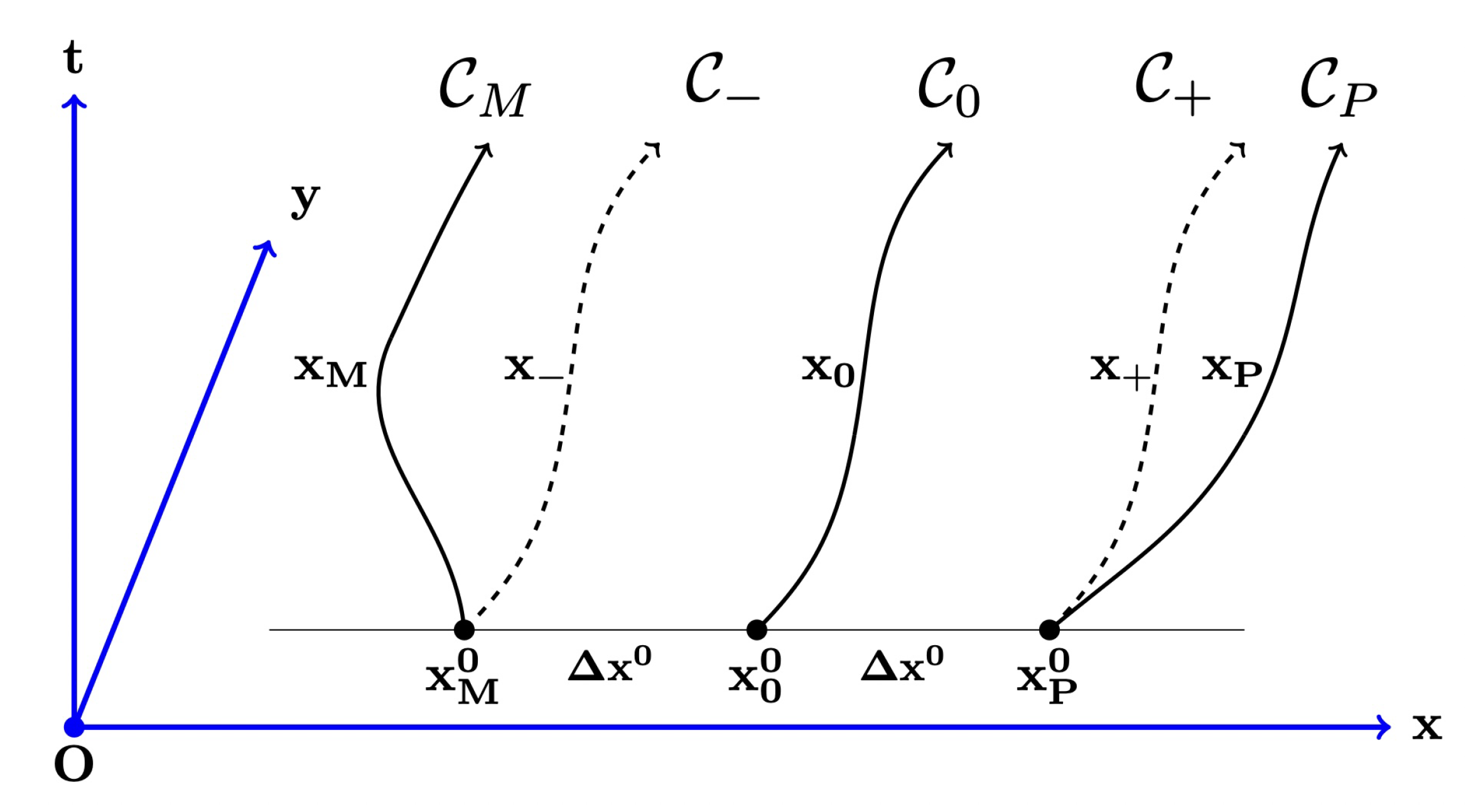
We consider a general equation written in Lagrangian form

$$\frac{\mathrm{d}\mathit{X}}{\mathrm{d}t}+\mathit{L}\mathit{X}+\mathit{N}\left(\mathit{X}\right)=0$$

(1)

where $\mathit{L}\mathit{X}$ are the linear terms and $\mathit{N}\left(\mathit{X}\right)$ are the nonlinear terms. Before we convert this grid-point equation to the spectral domain, we discretise it in time using a three time-level Lagrangian scheme. For a trajectory from departure point D at time $(n-1)\Delta t$ through arrival point A at $(n+1)\Delta t$, the equations are

$$\frac{{\mathit{X}}_A^{+}-{\mathit{X}}_D^{-}}{2\Delta t}+\mathit{L}\frac{{\mathit{X}}_A^{+}+{\mathit{X}}_D^{-}}{2}+{\mathit{N}}_M^0=0$$

where nonlinear terms are evaluated at the midpoint M and superscripts −, 0 and + denote values at times $(n-1)\Delta t$, $n\Delta t$ and $(n+1)\Delta t$. We can write the solution at the advanced time as

$${\mathit{X}}_A^{+}={[\mathit{I}+\Delta t\mathit{L}]}^{-1}\left\{(\mathit{I}-\Delta t\mathit{L}){\mathit{X}}_D^{-}-2\Delta t{\mathit{N}}_M^0\right\},$$

(2)

where the right hand side may be computed from known quantities. We now convert Equation (2) to spectral form, multiplying by ${\mathit{Y}}_n^m(\lambda ,\varphi )$ and integrating over the sphere to get

$${\mathit{x}}^{+}={(\mathit{I}+\Delta t\mathit{L})}^{-1}\left\{(\mathit{I}-\Delta t\mathit{L}){\mathit{x}}_D^{-}-2\Delta t{\mathit{n}}_M^0\right\},$$

where $\mathit{x}={\mathit{x}}_n^m$ is the vector of spherical harmonic coefficients of $\mathit{X}$, and $\mathit{n}={\mathit{n}}_n^m$ is similarly related to $\mathit{N}$. The right hand side may be computed from known quantities. We note that the linear operator $\mathit{L}$ commutes with the spectral transform.

2.2. Outline of the LaLT Scheme

We consider again the general equation in Lagrangian form (1). Before converting this grid-point equation to the spectral domain, we take the Laplace transform $\mathcal{L}$ along the trajectory starting from the departure point D at time $(n-1)\Delta t$:

$$s\widehat{\mathit{X}}-{\mathit{X}}_D^{-}+\widehat{\mathit{L}\mathit{X}}+\frac{{\mathit{N}}_M^0}{s}=0,$$

where s is the complex variable conjugate to t and $\widehat{\mathit{X}}:=\mathcal{L}\mathit{X}$. As for the LaSI scheme, we assume that the nonlinear term varies slowly, and approximate it by its value at the mid-point of the trajectory from $(D,(n-1)\Delta t)$ to $(A,(n+1)\Delta t)$.

To get an equation for $\widehat{\mathit{X}}$ we have to change the order of the Laplace transform and the linear operator $\mathit{L}$; in general, these do not commute. We define the commutator

$$\mathbf{\Gamma }:=[\mathcal{L},\mathit{L}]=\mathcal{L}\mathit{L}-\mathit{L}\mathcal{L}$$

so that the term $\widehat{\mathit{L}\mathit{X}}=\mathcal{L}\left\{\mathit{L}\mathit{X}\right\}$ becomes $\mathit{L}\widehat{\mathit{X}}+\mathbf{\Gamma }\left(\mathit{X}\right)$, and write the transformed equation

$$s\widehat{\mathit{X}}-{\mathit{X}}_D^{-}+\mathit{L}\widehat{\mathit{X}}+{\mathbf{\Gamma }}_M^0+\frac{{\mathit{N}}_M^0}{s}=0.$$

For computation of the commutator, see Appendix A.

We now convert to spectral form, integrating over the sphere, to get

$$s\widehat{\mathit{x}}-{\mathit{x}}_D^{-}+\mathit{L}\widehat{\mathit{x}}+{\gamma }_M^0+\frac{{\mathit{n}}_M^0}{s}=0,$$

where $\widehat{\mathit{x}}={\widehat{\mathit{x}}}_n^m$ is the vector of spherical harmonic coefficients of $\widehat{\mathit{X}}$, ${\mathit{x}}_D^{-}$ are the coefficients of ${\mathit{X}}_D^{-}$, and $\gamma ={\gamma }_n^m$ and $\mathit{n}={\mathit{n}}_n^m$ are the coefficients of $\mathbf{\Gamma }$ and $\mathit{N}$. The solution may be written

$$\widehat{\mathit{x}}={(s\mathit{I}+\mathit{L})}^{-1}\left({\mathit{x}}_D^{-}-{\gamma }_M^0-\frac{{\mathit{n}}_M^0}{s}\right)$$

where, after inverse transformation to the time domain, the right hand side may be computed from known quantities.

2.3. Accuracy Analysis

An accuracy analysis of the Laplace transform (LT) and semi-implicit (SI) schemes was presented in [5]. The main conclusions are reviewed here. Considering a simple oscillation equation

$$\frac{\partial X}{\partial t}=i\omega X+N\left(X\right)$$

(3)

that represents a component of the full system used in numerical weather prediction, the analysis showed that LT is more accurate than SI for both the linear and nonlinear terms. Assuming that the nonlinear term varies slowly, we take it to be a constant $\overline{N}$. The exact solution of (3) at time $(n+1)\Delta t$ is then

$$X^{+}=\left[exp(2i\omega \Delta t)\right]X^{-}+\left[\frac{exp(2i\omega \Delta t)-1}{i\omega }\right]\overline{N}$$

(4)

where $X^{-}$ is the solution at time $(n-1)\Delta t$.

The SI approximation to (3) is

$$\frac{X^{+}-X^{-}}{2\Delta t}=i\omega \frac{X^{+}+X^{-}}{2}+\overline{N}$$

Solving for the new value $X^{+}$, we have

$$X^{+}=\left(\frac{1+i\omega \Delta t}{1-i\omega \Delta t}\right)X^{-}+\left(\frac{1}{1-i\omega \Delta t}\right)2\Delta t\overline{N}$$

(5)

Comparing this with the exact solution (4), we find that both the linear and nonlinear components of the solution are misrepresented. For the exact solution (4), $X^{-}$ is multiplied by $exp(2i\omega \Delta t)$, while for the SI solution (5) the multiplier is

$$\rho =\left[\frac{1+i\omega \Delta t}{1-i\omega \Delta t}\right].$$

Thus, although there is no amplification, the phase error increases with $\omega \Delta t$. For the nonlinear term, the SI scheme has both modulus and phase errors; for details, see Section 2 in [5]. The errors in the SI scheme are significant when the time step is large.

We now apply the Laplace Transform $\mathcal{L}$ to Equation (3), taking the origin of time to be $(n-1)\Delta t$. The transform of (3) is

$$s\widehat{X}-X^{-}=i\omega \widehat{X}+\frac{\overline{N}}{s}.$$

The solution for $\widehat{X}$ follows immediately:

$$\widehat{X}=\frac{X^{-}}{s-i\omega }+\frac{\overline{N}}{s(s-i\omega )}.$$

(6)

The inverse Laplace transform ${\mathcal{L}}^{-1}$ with time set to $2\Delta t$ yields $X^{+}$ equal to the exact solution (4) at time $(n+1)\Delta t$. Thus, to the extent that the nonlinear term can be regarded as constant, the LT scheme is free from error.

2.4. Filtering with the LT Scheme

The LT scheme filters high frequency components by using a modified inversion operator ${\mathcal{L}}^{*}$: this can be done numerically by distorting the Bromwich contour for the inversion integral to a closed curve excluding poles associated with the high frequencies, as in [7,8,9,10,11]. In the present study, as in those of Lynch and Clancy [4] and Harney and Lynch [5], we invert the transform analytically, explicitly eliminating components with frequency greater than a specified cut-off frequency ${\omega }_c$.

Filtering may be done with a sharp cut-off at ${\omega }_c$, or with a smooth function such as a Butterworth filter having frequency response function

$$\mathcal{H}\left(\omega \right)=\frac{1}{1+{(\omega /{\omega }_c)}^L}.$$

(7)

Formally, we can define the modified inversion operator as the composition of the filter and the inverse Laplace transform: ${\mathcal{L}}^{*}={\mathcal{L}}^{-1}\circ \mathcal{H}$. In the numerical tests reported in Section 4 we set $L=16$ and choose the cut-off period ${\tau }_c=1$ h and ${\omega }_c=2\pi /{\tau }_c$. These values were chosen on the basis of many tests which showed that they yielded the best results for the given model resolution. Assuming that $\left|\omega \right|\ll {\omega }_c$, the inverse Laplace transform of (6) at time $(n+1)\Delta t$ gives

$$X^{+}=\left[exp(2i\omega \Delta t)\right]X^{-}+\left[\frac{exp(2i\omega \Delta t)-1}{i\omega }\right]\overline{N}.$$

(8)

This agrees with the exact analytic result (4) for both the linear and nonlinear terms.

Equation (8) is formally identical to Equation (4) in Cox and Matthews [12], for which the local truncation error is $\frac{1}{2}\Delta t^2{(\mathrm{d}N/\mathrm{d}t)}_n$. Assuming that the nonlinear term varies slowly, we have $\mathrm{d}N/\mathrm{d}t=O(\Delta t)$, and the local truncation error is third order in time. We note that (8) is also equivalent to a component of the vector Equation (2) in Clancy and Pudykiewicz [13]. For the relationship between Laplace transform integration and exponential integrators, see Appendix B.

3. Laplace Transforming the Peak Equations

We now describe the application of the Laplace transform scheme to the Peak model equations. We begin with Equations (9.38)–(9.41) in Section 9.3 of Ehrendorfer [6], but written in Lagrangian form:

$$\begin{array}{ccc}\hfill \frac{\mathrm{d}\mathit{\zeta }}{\mathrm{d}t}& =& {\mathit{F}}_{\mathit{\zeta }}-\varsigma \mathit{\zeta }\hfill \end{array}$$

(9)

$$\begin{array}{ccc}\hfill \frac{\mathrm{d}\mathit{\delta }}{\mathrm{d}t}& =& {\mathit{F}}_{\mathit{\delta }}-{\mathbf{\nabla }}_{\sigma }^2(R\overline{\mathit{T}}\pi +{\mathsf{\Phi }}_{\mathrm{S}}+\mathsf{G}\mathit{T})-\varsigma \mathit{\delta }\hfill \end{array}$$

(10)

$$\begin{array}{ccc}\hfill \frac{\mathrm{d}\mathit{T}}{\mathrm{d}t}& =& {\mathit{F}}_{\mathit{T}}-\mathsf{H}\mathit{\delta }-\varsigma \mathit{T}\hfill \end{array}$$

(11)

$$\begin{array}{ccc}\hfill {\mathit{p}}^{\mathrm{T}}\frac{\mathrm{d}\mathbf{\Pi }}{\mathrm{d}t}& =& -{\mathit{p}}^{\mathrm{T}}\mathit{\delta }\hfill \end{array}$$

(12)

The notation is generally conventional and equations similar to these have appeared frequently, going back to Hoskins and Simmons [14]. The dependent variables are vorticity ($\mathit{\zeta }$), divergence ($\mathit{\delta }$), temperature ($\mathit{T}$) and log surface pressure $\pi =log(p_{\mathrm{S}}/p_{00}$), where $p_{00}={10}^5$ Pa is the reference pressure. All variables are in the spectral domain but, for compactness, we suppress the spectral indices so that, for example, ${\mathit{\zeta }}_{\ell }^m$ is written simply as $\mathit{\zeta }$. Bold-face variables are vectors with values at all $\mathcal{M}$ model levels, which are equally spaced in $\sigma$-coordinates. The explicit expressions for the matrices $\mathsf{G}$ and $\mathsf{H}$ are given in Ehrendorfer [6] and vectors are defined as follows: ${\mathit{p}}^{\mathrm{T}}=(\Delta {\sigma }_1,\Delta {\sigma }_2,\cdots \Delta {\sigma }_{\mathcal{M}})$, $\mathbf{\Pi }=(\pi ,\pi ,\cdots ,\pi )$ and $\overline{\mathit{T}}=(\overline{T},\overline{T},\cdots ,\overline{T})$. Linear damping with coefficient $\varsigma$ may be applied to all variables except the surface pressure. The surface orography is represented by ${\mathsf{\Phi }}_{\mathrm{S}}$.

Diffusion is generally required to control spurious oscillations. Explicit diffusion schemes may become unstable for large time steps. To avoid this problem, we may use a scheme that is fully implicit. However, when combined with the Laplace transform scheme, this leads to additional complications. To circumvent these, we employ an operator splitting method. In the first stage, the inviscid Equations (9)–(12) with $\varsigma =0$, are advanced to time $(n+1)\Delta t$. This is then followed by a second stage in which the damping terms are integrated analytically (see Section 3.8).

3.1. Lagrangian Departure Points and Values

The Cartesian coordinates of a grid point at latitude $\varphi$ and longitude $\lambda$ are

$$X_A=rcos\lambda cos\varphi ,Y_A=rsin\lambda cos\varphi ,Z_A=rsin\varphi .$$

(13)

We compute $(X_A,Y_A,Z_A)$ for each grid-point and store them; they are independent of the model level. We use a method described by McGregor [15] to determine the departure points $(X_D,Y_D,Z_D)$. The inverse transformation is

$$r=\sqrt{X_D^2+Y_D^2+Z_D^2},\varphi =arcsin{Z}_D/r,\lambda =arctan(Y_D/X_D).$$

(14)

(We use the Fortran function atan2$(Y_D,X_D)$ here). The inverse transform must be done every time step, as the departure points change. They also depend on the model level.

Values of the variables at the departure points are obtained by interpolation in $(\lambda ,\varphi )$ space. A bicubic interpolation scheme is used. To facilitate interpolation, the grid point arrays are extended by two rows or columns around the boundaries. In the east–west direction, the extension is cyclic. At the poles, we repeat the two boundary rows, reversing their order and shifting the longitude by ${180}^{\circ }$ to allow for crossing the poles [15].

3.2. Orography

Preliminary tests with real data produced instabilities that were insensitive to damping and to spectral truncation. The problem first became manifest over the Andes and Himalayas. As is well known, orography can lead to problems with semi-Lagrangian integration schemes. Ritchie and Tanguay [16] proposed a modification that alleviates this problem. An orographic term is subtracted from the pressure, yielding a much smoother field that is more accurately interpolated to the departure points.

The method of Ritchie and Tanguay is used in the IFS model and described in the documentation [17]. The variable $\pi =log{p}_{\mathrm{S}}/p_{00}$ in (12) is separated into a constant part involving the orography and a variable part independent of orography:

$$\pi =\overline{\pi }+{\pi }^{\prime }$$

(15)

where $\overline{\pi }=-{\mathsf{\Phi }}_S/R\overline{T}$ is, by definition, the value for an isothermal hydrostatic atmosphere. Thus, $\mathbf{\nabla }\overline{\pi }=-(1/R\overline{T})\mathbf{\nabla }{\mathsf{\Phi }}_S$. We can then write

$${\left(\frac{\mathrm{d}\pi }{\mathrm{d}t}\right)}_k={\left(\frac{\mathrm{d}{\pi }^{\prime }}{\mathrm{d}t}\right)}_k+{\left({\mathit{F}}_{\pi }\right)}_k,\mathrm{where}{\left({\mathit{F}}_{\pi }\right)}_k=-\left[\frac{1}{R\overline{T}}{\mathit{V}}_k·\mathbf{\nabla }{\mathsf{\Phi }}_S\right].$$

(16)

The term ${\mathit{F}}_{\pi }$ involving the gradient of orography is computed in an Eulerian manner, and the continuity Equation (12) becomes

$$\frac{\mathrm{d}{\pi }^{\prime }}{\mathrm{d}t}={\mathit{p}}^{\mathrm{T}}({\mathit{F}}_{\pi }-\mathit{\delta }).$$

The advected variable ${\pi }^{\prime }$ is much smoother than the original variable $\pi$ since the underlying orography has been extracted.

3.3. Inviscid Stage

We integrate the equations using a split scheme, where the diffusion is omitted in the first stage and integrated analytically in the second. The nonlinear terms are evaluated at the central time and averaged between the departure and arrival points:

$${\mathit{F}}_M^0=\frac{1}{2}({\mathit{F}}_D^0+{\mathit{F}}_A^0).$$

This averaging is similar to the approach adopted in the ECMWF IFS model [17].

We now take the Laplace transform of (10)–(12), after applying (15) to change the pressure variable. Since the Laplace operator $\mathcal{L}$ does not commute with the spacial Laplacian ${\mathbf{\nabla }}_{\sigma }^2$, we introduce the commutator

$$\mathbf{\Gamma }:=s^2[\mathcal{L},{\mathbf{\nabla }}_{\sigma }^2](R\overline{\mathit{T}}{\pi }^{\prime }+\mathsf{G}\mathit{T})$$

(17)

The factor $s^2$ is included here to ensure that $\mathbf{\Gamma }$ is independent of s (see Appendix A). The transformed equations may be written

$$\begin{array}{ccc}\hfill s\widehat{\mathit{\delta }}& =& {\left({\mathit{F}}_{\mathit{\delta }}\right)}_M^0/s-{\mathbf{\Gamma }}_M^0/s^2+{\mathit{\delta }}_D^{-}-{\mathbf{\nabla }}_{\sigma }^2(R\overline{\mathit{T}}{\widehat{\pi }}^{\prime }+\mathsf{G}\widehat{\mathit{T}})\hfill \end{array}$$

(18)

$$\begin{array}{ccc}\hfill s\widehat{\mathit{T}}& =& {\left({\mathit{F}}_{\mathit{T}}\right)}_M^0/s-\mathsf{H}\widehat{\mathit{\delta }}+{\mathit{T}}_D^{-}\hfill \end{array}$$

(19)

$$\begin{array}{ccc}\hfill s{\widehat{\pi }}^{\prime }& =& {\mathit{p}}^{\mathrm{T}}[{\left({\mathit{F}}_{\pi }\right)}_A^0-\widehat{\mathit{\delta }}]+{\mathit{p}}^{\mathrm{T}}{\mathbf{\Pi }}_D^{-}\hfill \end{array}$$

(20)

Using the equations for $\widehat{\mathit{T}}$ and ${\widehat{\pi }}^{\prime }$, these quantities are eliminated from the divergence equation to obtain an equation for a single variable, $\widehat{\mathit{\delta }}$:

$$\begin{array}{ccc}\hfill s^2\widehat{\mathit{\delta }}& =& {\left({\mathit{F}}_{\mathit{\delta }}\right)}_M^0-{\mathbf{\nabla }}_{\sigma }^2(R\overline{\mathit{T}}s{\widehat{\pi }}^{\prime }+\mathsf{G}s\widehat{\mathit{T}})-{\mathbf{\Gamma }}_M^0/s+s{\mathit{\delta }}_D^{-}\hfill \\ & =& {\left({\mathit{F}}_{\mathit{\delta }}\right)}_M^0-{\mathbf{\nabla }}_{\sigma }^2[-R\overline{\mathit{T}}{\mathit{p}}^{\mathrm{T}}\widehat{\mathit{\delta }}+{\mathit{p}}^{\mathrm{T}}{\mathbf{\Pi }}_D^{\prime -})]\hfill \\ & & -{\mathbf{\nabla }}_{\sigma }^2\left[\mathsf{G}({\left({\mathit{F}}_{\mathit{T}}\right)}_M^0/s-\mathsf{H}\widehat{\mathit{\delta }}+{\mathit{T}}_D^{-})\right]-{\mathbf{\Gamma }}_M^0/s+s{\mathit{\delta }}_D^{-}\hfill \end{array}$$

We transfer all terms involving $\widehat{\mathit{\delta }}$ to the left:

$$\begin{array}{ccc}\hfill [s^2\mathsf{I}& -& {\mathbf{\nabla }}_{\sigma }^2(R\overline{\mathit{T}}{\mathit{p}}^{\mathrm{T}}+\mathsf{G}\mathsf{H})]\widehat{\mathit{\delta }}\hfill \\ & =& {\left({\mathit{F}}_{\mathit{\delta }}\right)}_M^0-{\mathbf{\Gamma }}_M^0/s+s{\mathit{\delta }}_D^{-}-{\mathbf{\nabla }}_{\sigma }^2[R\overline{\mathit{T}}{\mathit{p}}^{\mathrm{T}}{\mathbf{\Pi }}_D^{\prime -}+\mathsf{G}{\left({\mathit{F}}_{\mathit{T}}\right)}_M^0/s+\mathsf{G}{\mathit{T}}_D^{-}]\hfill \end{array}$$

(21)

3.4. Transforming to Vertical Eigenmodes

We now define the vertical structure matrix

$$\mathsf{B}:=R\overline{\mathit{T}}{\mathit{p}}^{\mathrm{T}}+\mathsf{G}\mathsf{H}.$$

Since $\mathsf{B}$ is symmetric, its eigen-structure can be written

$$\mathsf{B}\mathsf{E}=\mathsf{E}\mathsf{\Lambda }\mathrm{o}\mathrm{r}{\mathsf{E}}^{\mathrm{T}}\mathsf{B}\mathsf{E}=\mathsf{\Lambda }\mathrm{o}\mathrm{r}\mathsf{B}=\mathsf{E}\mathsf{\Lambda }{\mathsf{E}}^{\mathrm{T}}$$

We now transform to vertical eigen-modes by multiplying (21) by ${\mathsf{E}}^{\mathrm{T}}$:

$$\begin{array}{ccc}& & \left[s^2\mathsf{I}-{\mathbf{\nabla }}_{\sigma }^2\left({\mathsf{E}}^{\mathrm{T}}\mathsf{B}\mathsf{E}\right)\right]\left({\mathsf{E}}^{\mathrm{T}}\widehat{\mathit{\delta }}\right)=\hfill \\ & & {\mathsf{E}}^{\mathrm{T}}\left\{{\left({\mathit{F}}_{\mathit{\delta }}\right)}_M^0-{\mathbf{\Gamma }}_M^0/s+s{\mathit{\delta }}_D^{-}-{\mathbf{\nabla }}_{\sigma }^2[R\overline{\mathit{T}}{\mathit{p}}^{\mathrm{T}}{\mathbf{\Pi }}_D^{\prime -}+\mathsf{G}{\left({\mathit{F}}_{\mathit{T}}\right)}_M^0/s+\mathsf{G}{\mathit{T}}_D^{-}]\right\}.\hfill \end{array}$$

(22)

We note that, for a specific spectral component with total wavenumber ℓ, the Laplacian has a simple form $-{\mathbf{\nabla }}_{\sigma }^2=\ell (\ell +1)/a^2$. Then, defining ${\mathsf{\Omega }}^2:=-{\mathbf{\nabla }}_{\sigma }^2\mathsf{\Lambda }$, the matrix on the left hand side of (22) is

$$[s^2\mathsf{I}-{\mathbf{\nabla }}_{\sigma }^2\left({\mathsf{E}}^{\mathrm{T}}\mathsf{B}\mathsf{E}\right)]=[s^2\mathsf{I}-{\mathbf{\nabla }}_{\sigma }^2\mathsf{\Lambda }]=[s^2\mathsf{I}+{\mathsf{\Omega }}^2]$$

Since this is a diagonal matrix, the equation falls into $\mathcal{M}$ separate scalar equations, one for each vertical mode. We group the right hand terms of (22) according to powers of s:

$$\mathrm{RHS}={\mathsf{E}}^{\mathrm{T}}\left\{\mathcal{A}\times s+\mathcal{B}\times 1+\mathcal{C}\times (1/s)\right\}$$

(23)

where the vectors $\mathcal{A}$, $\mathcal{B}$ and $\mathcal{C}$ are

$$\begin{array}{ccc}\hfill \mathcal{A}& =& {\mathit{\delta }}_D^{-}\hfill \\ \hfill \mathcal{B}& =& {\left({\mathit{F}}_{\mathit{\delta }}\right)}_M^0-{\mathbf{\nabla }}_{\sigma }^2(R\overline{\mathit{T}}{\mathit{p}}^{\mathrm{T}}{\mathbf{\Pi }}_D^{\prime -}+\mathsf{G}{\mathit{T}}_D^{-})\hfill \\ \hfill \mathcal{C}& =& -{\mathbf{\nabla }}_{\sigma }^2\left(\mathsf{G}{\left({\mathit{F}}_{\mathit{T}}\right)}_M^0\right)-{\mathbf{\Gamma }}_M^0+{\mathbf{\nabla }}_{\sigma }^2{\left(R\overline{\mathit{T}}{\mathit{F}}_{\pi }\right)}_A^0.\hfill \end{array}$$

Multiplying (22) by the inverse of the diagonal matrix $s^2\mathsf{I}+{\mathsf{\Omega }}^2$, the equation for the k-th component is

$${\left({\mathsf{E}}^{\mathrm{T}}{\widehat{\mathit{\delta }}}_A^{+}\right)}_k=\left[\frac{s}{s^2+{\mathsf{\Omega }}_k^2}\right]{\left({\mathsf{E}}^{\mathrm{T}}\mathcal{A}\right)}_k+\left[\frac{1}{s^2+{\mathsf{\Omega }}_k^2}\right]{\left({\mathsf{E}}^{\mathrm{T}}\mathcal{B}\right)}_k+\left[\frac{1}{s(s^2+{\mathsf{\Omega }}_k^2)}\right]{\left({\mathsf{E}}^{\mathrm{T}}\mathcal{C}\right)}_k$$

(24)

We apply the operator ${\mathcal{L}}^{*}$ to (24), noting that the vertical transform and Laplace transform commute. The terms can be inverted using standard results from Laplace transform theory [18]. The value at time $(n+1)\Delta t$ is denoted by a + superscript:

$$\begin{array}{ccc}\hfill {\left({\mathsf{E}}^{\mathrm{T}}{\mathit{\delta }}_A^{+}\right)}_k& =& \left[\mathcal{H}\left({\mathsf{\Omega }}_k\right)cos2{\mathsf{\Omega }}_k\Delta t\right]{\left({\mathsf{E}}^{\mathrm{T}}\mathcal{A}\right)}_k\hfill \\ & & +\left[\frac{\mathcal{H}\left({\mathsf{\Omega }}_k\right)sin2{\mathsf{\Omega }}_k\Delta t}{{\mathsf{\Omega }}_k}\right]{\left({\mathsf{E}}^{\mathrm{T}}\mathcal{B}\right)}_k+\left[\frac{1-\mathcal{H}\left({\mathsf{\Omega }}_k\right)cos2{\mathsf{\Omega }}_k\Delta t}{{\mathsf{\Omega }}_k^2}\right]{\left({\mathsf{E}}^{\mathrm{T}}\mathcal{C}\right)}_k\hfill \end{array}$$

(25)

The filter response function $\mathcal{H}\left(\omega \right)$ was defined in Equation (7) above.

3.5. Inverse Vertical Transformation

Let us define four diagonal matrices

$$\begin{array}{ccc}\hfill {\mathsf{\Lambda }}_A& =& \mathrm{diag}\left(\mathcal{H}\left({\mathsf{\Omega }}_k\right)cos2{\mathsf{\Omega }}_k\Delta t\right)\hfill \\ \hfill {\mathsf{\Lambda }}_B& =& \mathrm{diag}\left(\frac{\mathcal{H}\left({\mathsf{\Omega }}_k\right)sin2{\mathsf{\Omega }}_k\Delta t}{{\mathsf{\Omega }}_k}\right)\hfill \\ \hfill {\mathsf{\Lambda }}_C& =& \mathrm{diag}\left(\frac{1-\mathcal{H}\left({\mathsf{\Omega }}_k\right)cos2{\mathsf{\Omega }}_k\Delta t}{{\mathsf{\Omega }}_k^2}\right)\hfill \\ \hfill {\mathsf{\Lambda }}_D& =& \mathrm{diag}\left(\frac{2{\mathsf{\Omega }}_k\Delta t-\mathcal{H}\left({\mathsf{\Omega }}_k\right)sin2{\mathsf{\Omega }}_k\Delta t}{{\mathsf{\Omega }}_k^3}\right)\hfill \end{array}$$

(${\mathsf{\Lambda }}_D$ will be needed below). Then (25) can be written

$${\mathsf{E}}^{\mathrm{T}}{\mathit{\delta }}_A^{+}={\mathsf{\Lambda }}_A{\mathsf{E}}^{\mathrm{T}}\mathcal{A}+{\mathsf{\Lambda }}_B{\mathsf{E}}^{\mathrm{T}}\mathcal{B}+{\mathsf{\Lambda }}_C{\mathsf{E}}^{\mathrm{T}}\mathcal{C}$$

(26)

We can now calculate the divergence at the advanced time,

$${\mathit{\delta }}_A^{+}=\mathsf{E}\left({\mathsf{E}}^{\mathrm{T}}{\mathit{\delta }}_A^{+}\right)=\mathsf{E}{\mathsf{\Lambda }}_A{\mathsf{E}}^{\mathrm{T}}\mathcal{A}+\mathsf{E}{\mathsf{\Lambda }}_B{\mathsf{E}}^{\mathrm{T}}\mathcal{B}+\mathsf{E}{\mathsf{\Lambda }}_C{\mathsf{E}}^{\mathrm{T}}\mathcal{C}$$

For compactness, we define the propagation matrices:

$$\begin{array}{ccc}\hfill {\mathsf{P}}_A=\mathsf{E}{\mathsf{\Lambda }}_A{\mathsf{E}}^{\mathrm{T}}& & {\mathsf{P}}_B=\mathsf{E}{\mathsf{\Lambda }}_B{\mathsf{E}}^{\mathrm{T}}\hfill \\ \hfill {\mathsf{P}}_C=\mathsf{E}{\mathsf{\Lambda }}_C{\mathsf{E}}^{\mathrm{T}}& & {\mathsf{P}}_D=\mathsf{E}{\mathsf{\Lambda }}_D{\mathsf{E}}^{\mathrm{T}}\hfill \end{array}$$

(${\mathsf{P}}_D$ will be used below). Then we can write the solution as

$${\mathit{\delta }}_A^{+}={\mathsf{P}}_A\mathcal{A}+{\mathsf{P}}_B\mathcal{B}+{\mathsf{P}}_C\mathcal{C}$$

(27)

The $\mathsf{P}$-matrices can be pre-computed and stored, since they do not depend on the model variables.

3.6. Temperature and Pressure

We return to Equations (19) and (20):

$$\begin{array}{ccc}\hfill s\widehat{\mathit{T}}& =& {\left({\mathit{F}}_{\mathit{T}}\right)}_M^0/s-\mathsf{H}\widehat{\mathit{\delta }}+{\mathit{T}}_D^{-}\hfill \\ \hfill s{\widehat{\pi }}^{\prime }& =& {\mathit{p}}^{\mathrm{T}}[{\left({\mathit{F}}_{\pi }\right)}_A^0-\widehat{\mathit{\delta }}]+{\mathit{p}}^{\mathrm{T}}{\mathbf{\Pi }}_D^{-}\hfill \end{array}$$

Noting that ${\mathcal{L}}^{*}\{1/s\}=1$ and ${\mathcal{L}}^{*}\{1/s^2\}=t$, dividing these equations by s and applying the operator ${\mathcal{L}}^{*}$ at time $2\Delta t$, we have

$$\begin{array}{ccc}\hfill {\mathit{T}}_A^{+}& =& {\mathit{T}}_D^{-}+2\Delta t{\left({\mathit{F}}_{\mathit{T}}\right)}_M^0-\mathsf{H}{\mathcal{L}}^{*}\left\{\widehat{\mathit{\delta }}/s\right\}\hfill \end{array}$$

(28)

$$\begin{array}{ccc}\hfill {\pi }_A^{\prime +}& =& {\mathit{p}}^{\mathrm{T}}{\mathbf{\Pi }}_D^{\prime -}+2\Delta t{\mathit{p}}^{\mathrm{T}}\left[{\left({\mathit{F}}_{\pi }\right)}_A^0-{\mathcal{L}}^{*}\left\{\widehat{\mathit{\delta }}/s\right\}\right].\hfill \end{array}$$

(29)

Both (28) and (29) require computation of

$$\tilde{\mathit{\delta }}={\mathcal{L}}^{*}\left\{\widehat{\mathit{\delta }}/s\right\}.$$

(30)

This term involves a convolution integral that may be approximated by the trapezoidal rule

$${\mathcal{L}}^{*}\left\{\widehat{\mathit{\delta }}/s\right\}={\int }_0^{2\Delta t}\mathit{\delta }\mathrm{d}t\approx 2\Delta t\left(\frac{{\mathit{\delta }}_D^{-}+{\mathit{\delta }}_A^{+}}{2}\right)=2\Delta t\overline{\mathit{\delta }}$$

where $\overline{\mathit{\delta }}$ is the average of old and new values of $\mathit{\delta }$. However, this method was found not to perform in a satisfactory manner. We therefore employed an alternative strategy: the term (30) was computed by noting that

$$\tilde{\mathit{\delta }}={\mathcal{L}}^{*}\left\{\widehat{\mathit{\delta }}/s\right\}=\mathsf{E}{\mathcal{L}}^{*}\left\{{\mathsf{E}}^{\mathrm{T}}\widehat{\mathit{\delta }}/s\right\}.$$

(31)

We divide (24) by s to give

$${\left(\frac{{\mathsf{E}}^{\mathrm{T}}\widehat{\mathit{\delta }}}{s}\right)}_k=\left[\frac{1}{s^2+{\mathsf{\Omega }}_k^2}\right]{\left({\mathsf{E}}^{\mathrm{T}}\mathcal{A}\right)}_k+\left[\frac{1}{s(s^2+{\mathsf{\Omega }}_k^2)}\right]{\left({\mathsf{E}}^{\mathrm{T}}\mathcal{B}\right)}_k+\left[\frac{1}{s^2(s^2+{\mathsf{\Omega }}_k^2)}\right]{\left({\mathsf{E}}^{\mathrm{T}}\mathcal{C}\right)}_k$$

(32)

We invert this using standard results for Laplace transforms to obtain

$$\begin{array}{ccc}\hfill {\mathcal{L}}^{*}{\left\{\frac{{\mathsf{E}}^{\mathrm{T}}\widehat{\mathit{\delta }}}{s}\right\}}_k& =& \left[\frac{\mathcal{H}\left({\mathsf{\Omega }}_k\right)sin2{\mathsf{\Omega }}_k\Delta t}{{\mathsf{\Omega }}_k}\right]{\left({\mathsf{E}}^{\mathrm{T}}\mathcal{A}\right)}_k+\left[\frac{1-\mathcal{H}\left({\mathsf{\Omega }}_k\right)cos2{\mathsf{\Omega }}_k\Delta t}{{\mathsf{\Omega }}_k^2}\right]{\left({\mathsf{E}}^{\mathrm{T}}\mathcal{B}\right)}_k\hfill \\ & & +\left[\frac{2{\mathsf{\Omega }}_k\Delta t-\mathcal{H}\left({\mathsf{\Omega }}_k\right)sin2{\mathsf{\Omega }}_k\Delta t}{{\mathsf{\Omega }}_k^3}\right]{\left({\mathsf{E}}^{\mathrm{T}}\mathcal{C}\right)}_k\hfill \end{array}$$

Then using the $\mathsf{\Lambda }$-matrices, we can write

$${\mathcal{L}}^{*}\left\{\frac{{\mathsf{E}}^{\mathrm{T}}\widehat{\mathit{\delta }}}{s}\right\}={\mathsf{\Lambda }}_B{\mathsf{E}}^{\mathrm{T}}\mathcal{A}+{\mathsf{\Lambda }}_C{\mathsf{E}}^{\mathrm{T}}\mathcal{B}+{\mathsf{\Lambda }}_D{\mathsf{E}}^{\mathrm{T}}\mathcal{C}$$

Noting (31) and using the $\mathsf{P}$-matrices, we can now write

$$\tilde{\mathit{\delta }}={\mathsf{P}}_B\mathcal{A}+{\mathsf{P}}_C\mathcal{B}+{\mathsf{P}}_D\mathcal{C}.$$

(33)

Finally, using (28) and (29), the values of $T_A^{+}$ and ${\pi }_A^{\prime +}$ are

$$\begin{array}{ccc}\hfill {\mathit{T}}_A^{+}& =& {\mathit{T}}_D^{-}+2\Delta t[{\left({\mathit{F}}_{\mathit{T}}\right)}_M^0-\mathsf{H}\tilde{\mathit{\delta }}/2\Delta t]\hfill \end{array}$$

(34)

$$\begin{array}{ccc}\hfill {\pi }_A^{\prime +}& =& {\mathit{p}}^{\mathrm{T}}{\mathbf{\Pi }}_D^{\prime -}+2\Delta t{\mathit{p}}^{\mathrm{T}}\left[{\left({\mathit{F}}_{\pi }\right)}_A^0-\tilde{\mathit{\delta }}/2\Delta t\right].\hfill \end{array}$$

(35)

3.7. Integrating the Vorticity

To complete the inviscid stage of the time step, we take the Laplace transform of the vorticity Equation (9)

$$s\widehat{\mathit{\zeta }}={\mathit{\zeta }}_D^{-}+{\left({\mathit{F}}_{\mathit{\zeta }}\right)}_M^0/s$$

Dividing by s and applying ${\mathcal{L}}^{*}$ at $2\Delta t$ yields

$${\mathit{\zeta }}_A^{+}={\mathit{\zeta }}_D^{-}+2\Delta t{\left({\mathit{F}}_{\mathit{\zeta }}\right)}_M^0,$$

(36)

which is a standard centred Lagrangian step along the trajectory. As the poles are at $s=0$, the Laplace transform has no filtering effect here.

As is usual with the leapfrog model, a Robert-Asselin filter [19] is applied to the prognostic variables to prevent separation of the solutions at odd and even time steps. The coefficient is fixed at $ϵ=0.03$ in all cases.

3.8. Diffusion Stage

The governing equation for a spectral component of any of the variables $\mathit{\delta }$, $\mathit{\zeta }$ or $\mathit{T}$ may be written in the form

$$\frac{\mathrm{d}\Psi }{\mathrm{d}t}=F-\varsigma \Psi$$

We split the right hand side into two parts and integrate them separately. We first integrate the inviscid equation

$$\frac{\mathrm{d}\Psi }{\mathrm{d}t}=F$$

over a time interval $2\Delta t$ with initial condition ${\Psi }^{-}$ and denote the result as ${\Psi }^{*}$. We then integrate the equation

$$\frac{\partial \Psi }{\partial t}=-\varsigma \Psi$$

analytically with the initial condition ${\Psi }^{*}$ to get

$${\Psi }^{+}=exp(-2\Delta t\varsigma ){\Psi }^{*}$$

which is the required solution at time $(n+1)\Delta t$. This second stage is applied to the divergence, vorticity and temperature; the surface pressure is not damped in this way.

The parameter $\varsigma$ depends only upon the horizontal scale. The diffusion is assumed to be of the form

$$\frac{\partial Q}{\partial t}={\nu }_2{\nabla }^{2}Q+{\nu }_6{\nabla }^{6}Q$$

(37)

In the spectral domain, the damping coefficient becomes

$$\varsigma =\left[{\nu }_2\left(\frac{\ell (\ell +1)}{a^2}\right)+{\nu }_6{\left(\frac{\ell (\ell +1)}{a^2}\right)}^3\right]$$

We note that the spectral equations are unchanged in form by the addition of the hyper-diffusion term (${\nu }_6$); only the value of the coefficient is changed. The ${\nu }_6$-term more strongly damps the smaller scales. Having applied diffusion, we have all the model variables at the advanced time, and a new time step can be taken.

4. Numerical Evaluation of the Integration Schemes

In this section, we describe a series of tests comparing simulations using the Laplace transform scheme (LaLT) and the semi-implicit scheme (LaSI). The LaSI and LaLT models were run with 20, 40 and 60 min time steps. For LaLT, a cut-off value ${\tau }_c=1$ h was set for all time steps. In most cases, the reference forecast was an integration of the LaSI model with a time step $\Delta t=10$ min.

Eulerian models are subject to a Courant-Friedrichs-Lewy stability condition. For an advection speed $\overline{u}=100$ m/s, the non-dimensional stability ratio $\overline{u}\Delta t/\mathit{\delta }x$ is unity for a time step $\Delta t=1500$ s or 25 min. In fact, both the Eulerian models, EuSI and EuLT, were found to be unstable for a time step of 24 min. The Lagrangian models are not subject to this limitation.

The horizontal resolution of the model was at triangular truncation $T85$. The colocation grid corresponding to this has $256\times 129$ grid points, with a grid interval of approximately 150 km. In all cases, there were 20 vertical levels, uniformly spaced in $\sigma$-coordinates.

The default setting of the diffusion coefficient was ${\nu }_2=7\times {10}^5$ m ${}^2$ s ${}^{-1}$: the damping of a component of total wavenumber ℓ is $\varsigma ={\nu }_2\ell (\ell +1)/a^2$ s ${}^{-1}$. The default value implies an e-folding time of 2.2 h for the shortest waves represented at truncation T85. Sixth order diffusion (${\nu }_6={10}^7$ m ${}^2$ s ${}^{-1}$) was also applied for runs with a 60 min time step. We note that LaLT consistently required less explicit diffusion than LaSI.

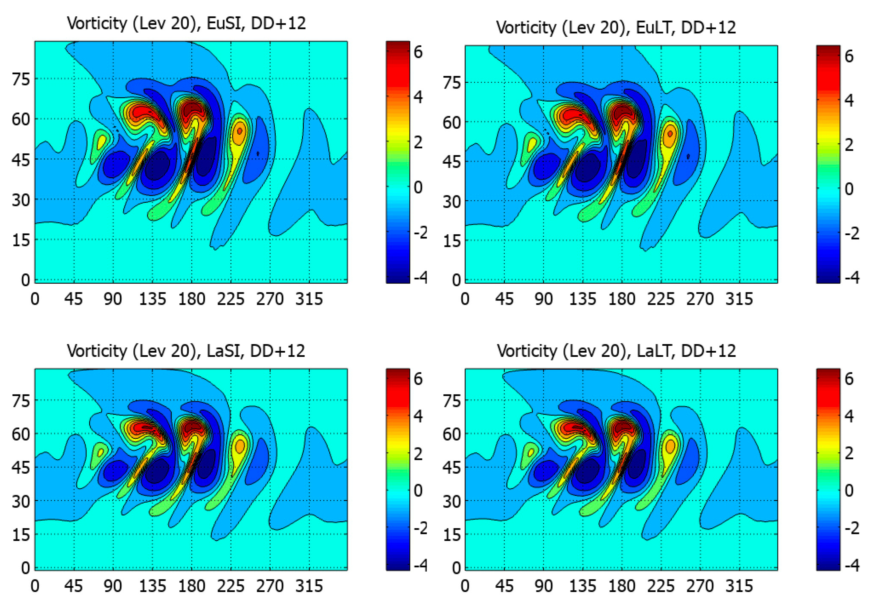
4.1. Initial Validation Tests

Numerous tests were carried out to confirm the correct operation of the model codes. For short time steps, the Eulerian and Lagrangian advection produced similar results, as did the semi-implicit and Laplace Transform adjustment. As an example of the performance of the four models, simulations of a growing baroclinically unstable disturbance [20] are shown in Figure 1. The initial field is a zonally symmetric flow with a small perturbation on the Greenwich meridian. The four models were integrated for 12 days, each with a time step $\Delta t=5$ min. The damping coefficient was ${\nu }_2=7\times {10}^5$ and all other parameter settings were equal for the four runs. The four simulations are quite similar, although we notice a slight damping for the Lagrangian runs, associated with the interpolations involved in the treatment of advection.

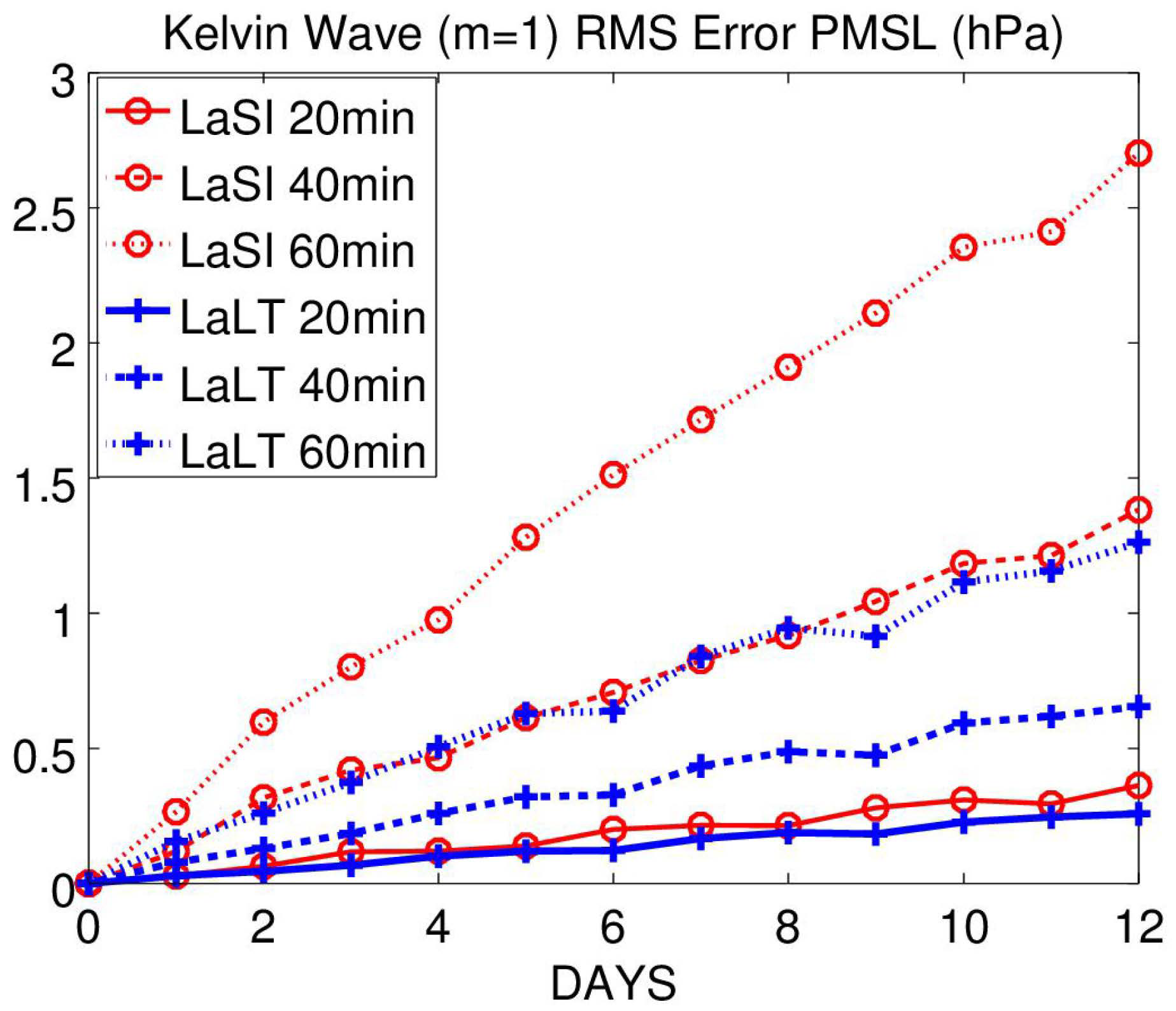
4.2. Kelvin Waves

Kelvin waves are eastward propagating waves that play an important role in atmospheric dynamics. Clancy and Lynch [7] showed that the LT scheme had a significantly smaller phase error than the semi-implicit scheme for the integration of these waves. Exact Kelvin Wave initial conditions can be generated using the method of Kasahara [21]. In this study, we use a simple analytical approximation described in [22]. We examine the solutions for zonal wave numbers 1 and 4. The wave amplitude is 100 m in both cases. The theoretical period for the Kelvin wave with zonal wavenumber $m=1$ is about 32 h and for $m=4$ is about 8.3 h ([21], Figure 9). Figure 2 shows that the root mean square errors for wavenumber 1 for LaLT (blue lines) are significantly smaller than for LaSI (red lines). Forecasts were run with time steps of 20, 40 and 60 min (solid, dashed and dotted lines, respectively).

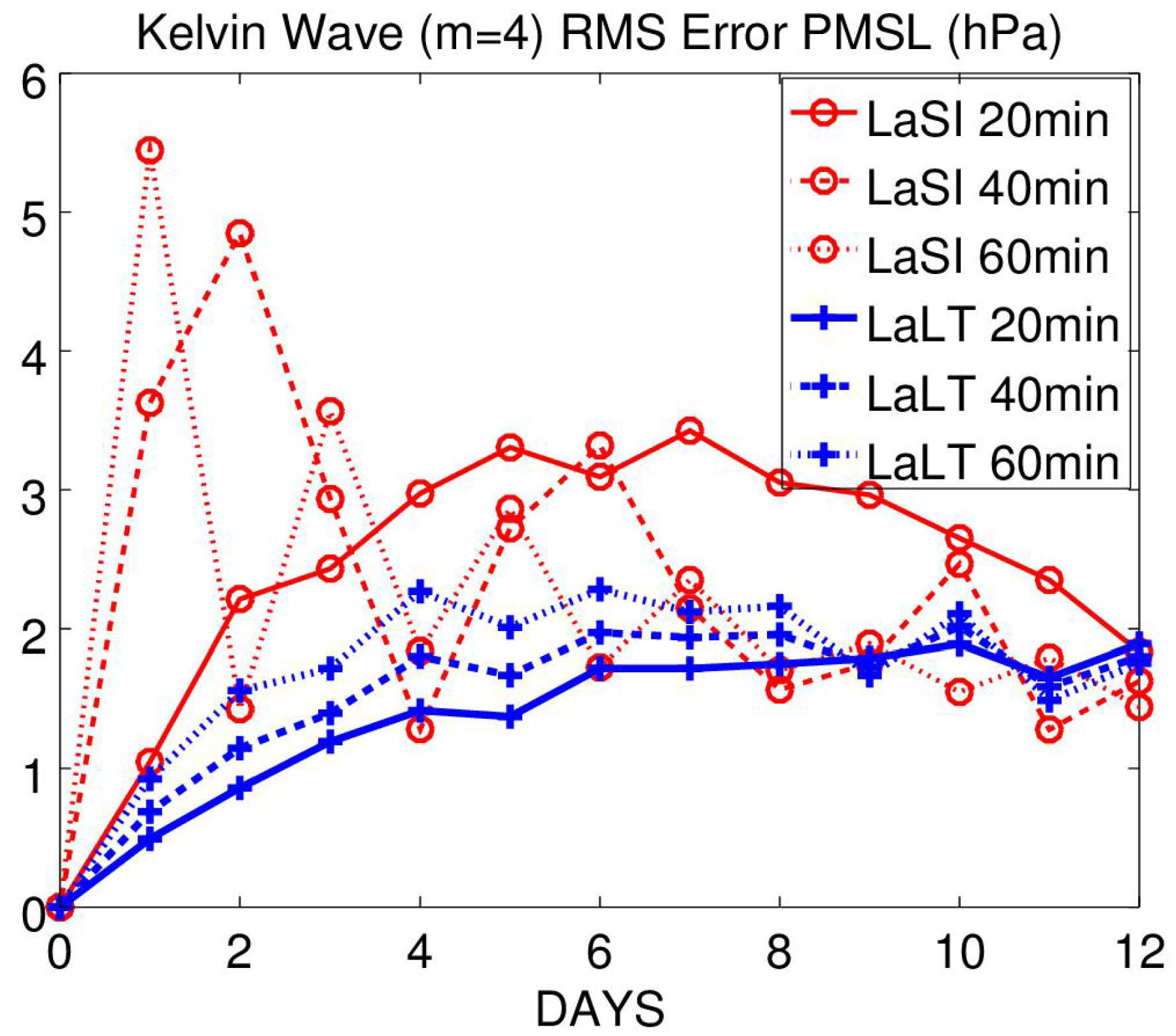
For the LaSI forecast of wave number 4 (Figure 3) with a 20 min step, the propagation of the wave lags by a full wavelength by the end of the integration, reducing the rms error. The errors for the LaSI scheme with the larger time steps oscillate wildly as the wave moves into and out of phase with the reference solution. The errors for LaLT are much smaller and behave in a more realistic and steady manner.

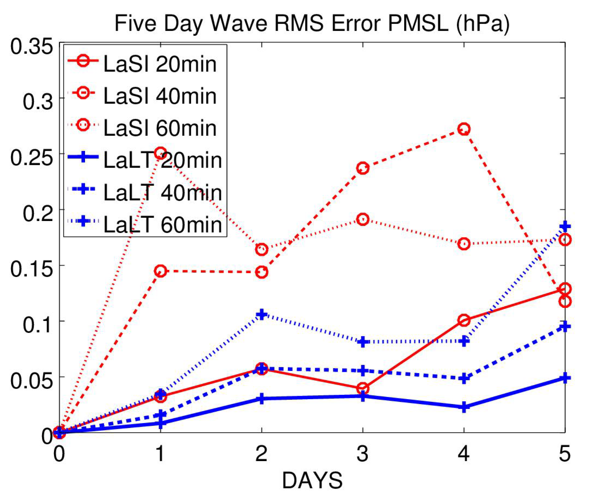
4.3. The Five-Day Wave

The Five-day Wave RO(1,2) is the gravest symmetric rotational Hough mode of zonal wavenumber 1. It is closely related to the initial state chosen by Lewis Fry Richardson for their preliminary shallow-water forecast experiment ([23], Section 4.1). The initial conditions for a three-dimensional Five-day Wave were implemented in Peak. The initial pressure amplitude was 10 hPa, with mean pressure 1000 hPa. As no zonal mean flow was included, the wave has a period close to 5 days. 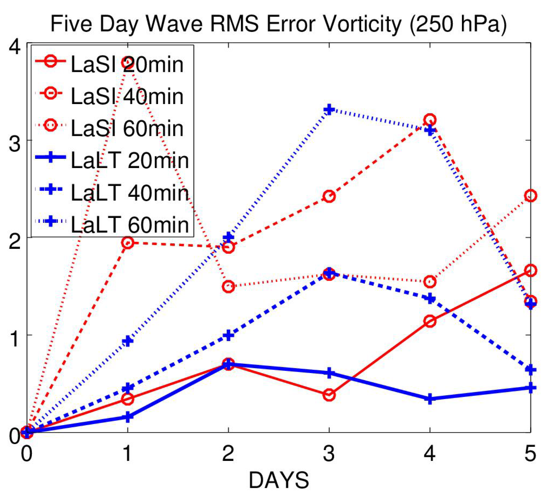Figure 4 shows the root mean square errors in surface pressure for the LaSI scheme (red) and the LaLT scheme (blue), with time steps of 20 min (solid lines), 40 min (dashed lines) and 60 min (dotted lines). The reference is an SI forecast with time step of 10 min. The error level for LaLT is significantly less than that of the LaSI scheme, especially for the longer time step. The scores for vorticity at 250 hPa (Figure 5) confirm the superior performance of LaLT.

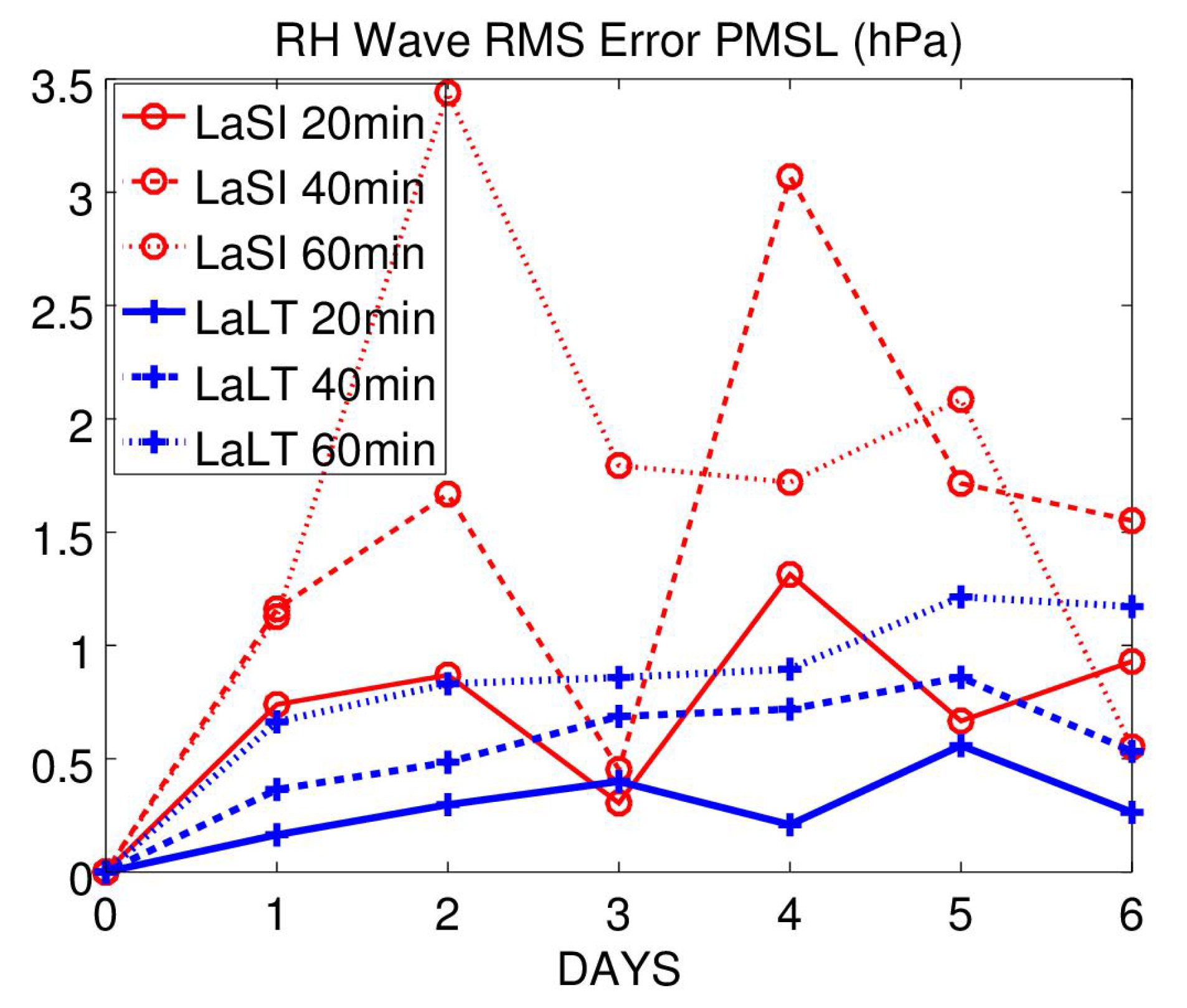
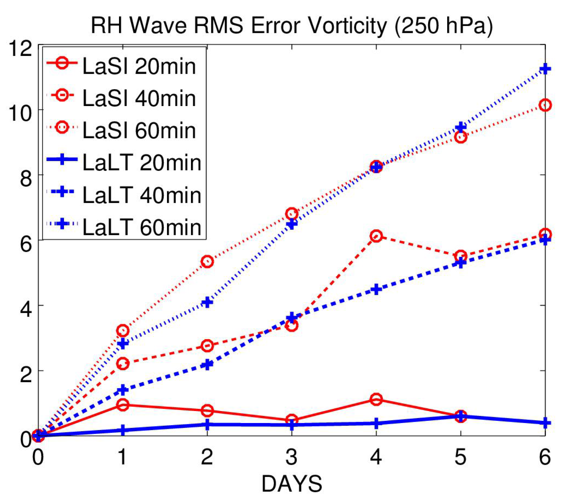
4.4. Rossby-Haurwitz Wave

Rossby-Haurwitz (RH) waves are exact solutions of the nonlinear barotropic vorticity equation. While they are not eigenfunctions of the shallow water equations, they have frequently been used as test cases. Following Phillips [24], the RH(4,5) wave was chosen as Test Case 6 by Williamson et al. [25]. This test case has been extended to three dimensions; the initial vorticity field is as in the barotropic case, the divergence is zero and a vertical temperature profile and surface pressure field are defined; for details, see [26].

The LaSI and LaLT schemes, with time steps of 20, 40 and 60 min, were compared to a reference run of LaSI using a time step of 10 s. No diffusion was used for the reference or LaLT runs, but the LaSI runs were unstable. This was overcome by applying horizontal diffusion with a coefficient ${\nu }_2=3\times {10}^6$ m ${}^2$ s ${}^{-1}$. Figure 6 shows the root mean square errors in surface pressure for the LaSI scheme (red) and the LaLT scheme (blue). The error level for LaLT is substantially less than for the LaSI scheme. Figure 7 shows scores for vorticity near the tropopause (250 hPa). The forecasts for LaSI and LALT have comparable errors, but there is a slight advantage for the Laplace transform scheme.

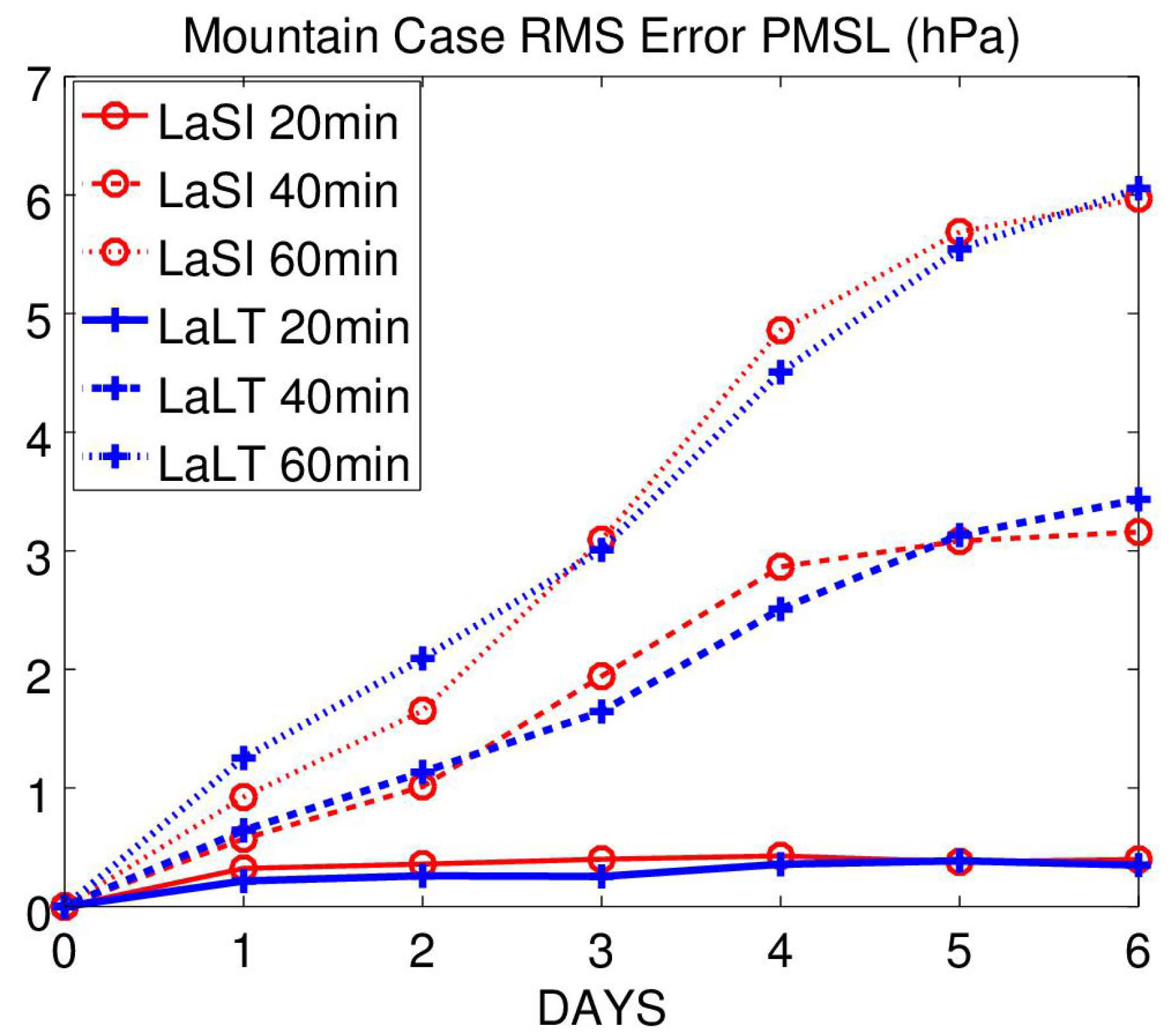
4.5. Flow over a Mountain

Test Case 5 of Williamson et al. [25] treats a zonal flow over an isolated mountain. The mountain is centred at $({90}^{\circ } \mathrm{E},{30}^{\circ } \mathrm{N})$ with maximum height 2000 m. No analytic solution is known so, as usual, we take the LaSI run with $\Delta t=10$ min as a reference. Figure 8 shows the root mean square errors in surface pressure for the LaSI scheme (red) and LaLT scheme (blue), with time steps of 20 min (solid), 40 min (dashed) and 60 min (dotted lines). The error levels for the two schemes are very close in value.

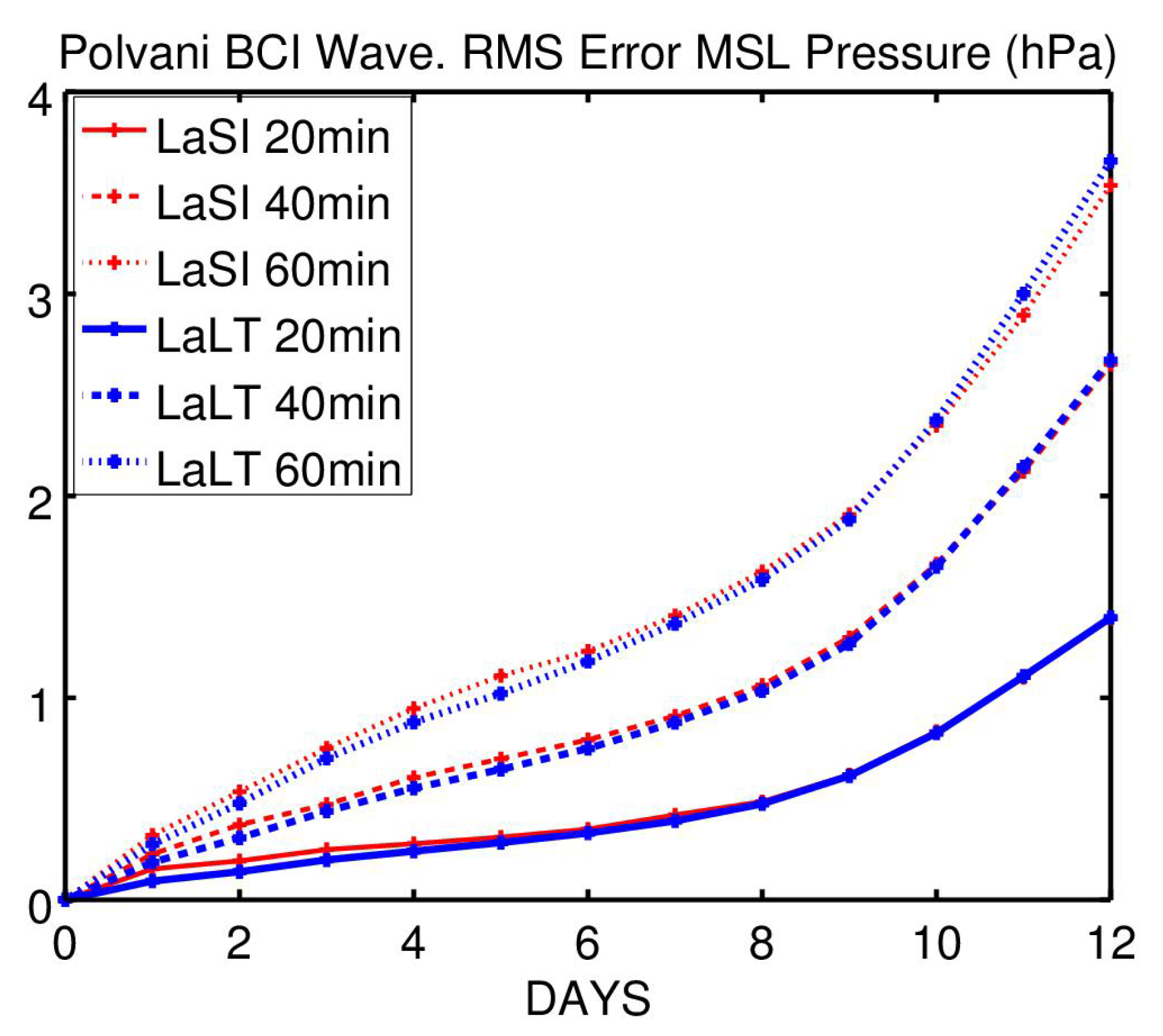
4.6. A Baroclinically Unstable Wave

Polvani et al. [20] devised a test case for baroclinic instability. The initial conditions consist of a non-divergent zonal flow with constant surface pressure. A small perturbation is added to the temperature to trigger the development of baroclinic instability. The test case of Polvani et al. was used by Ehrendorfer [6] to validate the Peak model. With a fixed value for the diffusion coefficient, the initial conditions are ‘numerically convergent’ as shown in [20] using two different numerical models. A test case quite similar to that of Polvani et al. was constructed by Jablonowski and Williamson [27].

We use the test case of Polvani et al. [20] to show that the LaLT scheme can accurately simulate baroclinic development. Using this case, Harney and Lynch [5] showed that the EuLT scheme can accurately simulate baroclinic development. In Figure 1, above, we showed the 12-day forecasts for all four schemes all with a small time step $\Delta t=5$ min. There was no substantive difference between the four schemes. They are also indistinguishable from the results plotted in ([20], Figure 4). Thus, all four schemes are capable of forecasting baroclinic development with high precision.

Quantitative scores confirm that the differences in performance are small: Figure 9 shows the root mean square errors in surface pressure (hPa) for forecasts with the LaSI scheme (red) and LaLT scheme (blue), with time steps 20, 40 and 60 min. As usual, the reference forecast is LaSI with a 10 min time step. It is clear that the time truncation error grows with forecast range. It is also clear that the error is greater for larger time steps. The important point is that the errors for the two integration schemes are very similar in magnitude.

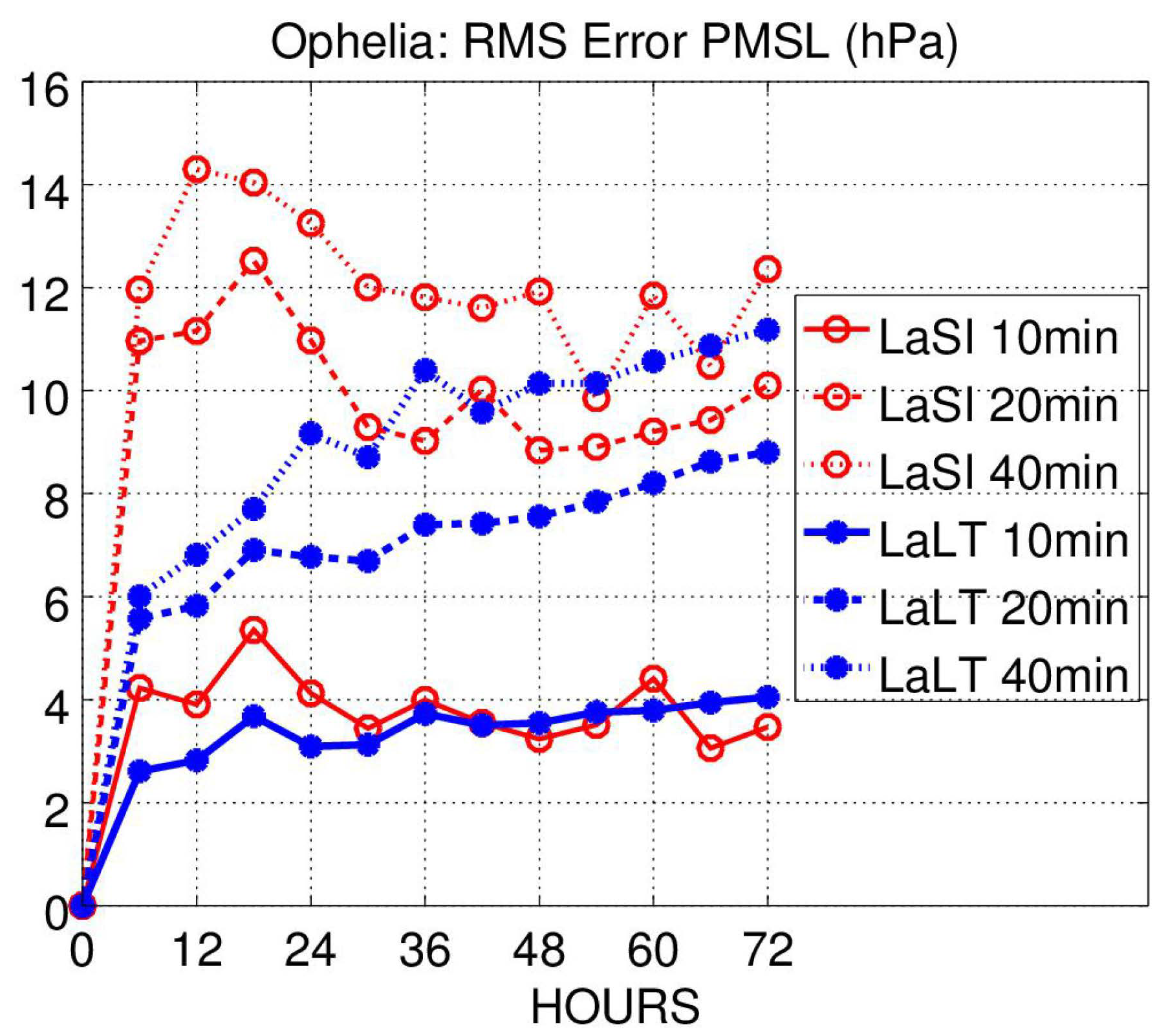
4.7. Real Data Test

The simple wave tests described above indicate superior accuracy for the LT scheme compared to the semi-implicit scheme. The ultimate conclusion on superiority of the scheme must involve comprehensive comparisons for a large range of meteorological conditions. As a first step, a single test using real atmospheric data is described here.

Data was retrieved from the European Centre for Medium-Range Weather Forecasts MARS archive. The date chosen was 00 UTC on 15 October 2017, the day before a major storm, Ophelia, reached Ireland. This data comprised temperature, divergence and vorticity fields on 25 pressure levels, surface pressure and the relevant orography field. These fields where interpolated onto the 20 sigma levels and reduced to the spectral resolution T85 used for the Peak forecasts. The process of interpolation introduced noise, which was removed by initialization, as described by Harney and Lynch [5]. Using initialized data, six forecasts were performed using the LaSI and LaLT schemes with time steps of 10, 20 and 40 min.

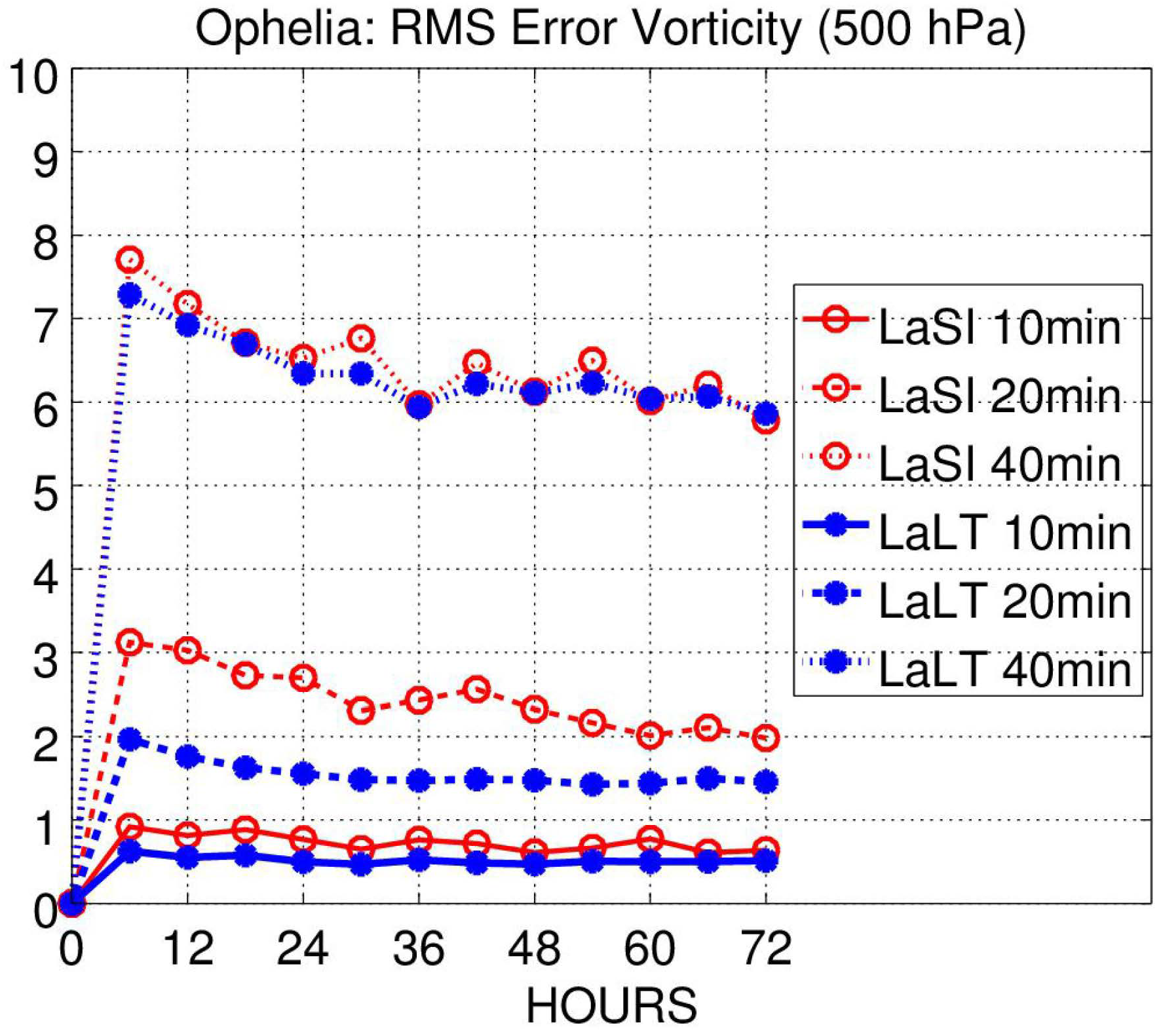
Figure 10 shows the root mean square error for surface pressure. The reference is a forecast using LaSI with a time step of 5 min. The red curves are for LaSI and the blue ones for LaLT. For the 10 min step, the errors are comparable for the two models, although the error during the initial day is smaller for LaLT. For the larger time steps, the Laplace transform scheme is clearly superior to the semi-implicit scheme. Scores for mid-troposphere vorticity (Figure 11) confirm the superior performance of LaLT.

5. Conclusions

An integration scheme using a Laplace transform for adjustment combined with a semi-Lagrangian advection scheme (LaLT) has been found to yield results at least as accurate as the popular semi-implicit semi-Lagrangian scheme. The numerical tests described in Section 4 clearly indicate the superior accuracy for the LaLT scheme compared to the semi-implicit scheme LaSI. The single experiment with real data reinforces this advantage.

Ultimate conclusions on the superiority of the LaLT scheme require more comprehensive comparisons for a large range of meteorological conditions. The potential for operational implementation of LaLT would depend upon more exhaustive testing with higher spatial resolution and incorporating a full package of physical processes.

There are well-known advantages of using a two time level scheme for Lagrangian advection. There appear to be no difficulties in principle combining such a scheme with Laplace transform adjustment.

The efficient formulation of the LaLT scheme, with analytical inversion of the Laplace transform, is made possible through the use of a spectral model. An active debate on the future of spectral models has been ongoing for decades. The global simulation of an entire season of the Earth’s atmosphere, with a 1 km grid and upper boundary of 80 km [28], suggests that spectral models will continue to be competitive in the future.

For practical reasons, the semi-Lagrangian method used in this study was applied only to the horizontal advection. However, there is no difficulty to include vertical advection in the scheme. The algorithmic complexity of the LaLT scheme is comparable to that of LaSI. Averaging over a range of integrations, the processing time for LaLT was just 6% more than for LaSI, so the Laplace transform scheme is computationally competitive.

In summary, the main result of this study is that the LaLT scheme is clearly superior in accuracy to the LaSI scheme for the large time steps typically used with semi-Lagrangian advection. The evidence presented gives a clear indication of the practical potential of the LaLT scheme for integrating weather and climate prediction models.