Radio Observations of Microquasars with FAST

Abstract

We report six radio observations of four microquasars—SS 433, GRS 1915+105, Cyg X-3 and MAXI J1820+070—conducted between 2022 and 2025 with the Five-hundred-meter Aperture Spherical radio Telescope (FAST) using its pulsar backend, achieving a time resolution of 98.304 $\mathsf{\mu }$s across an effective feed range of 1.04–1.45 GHz. A major focus of this work is the development of a standardized calibration pipeline for microquasar observations, including RFI mitigation, flux density, and polarization calibration, as well as multi-beam correlation inspections. Using On–Off mode and cross-beam verification, radio activity was detected in SS 433, GRS 1915+105 and Cyg X-3, while MAXI J1820+070 remained inactive. Both SS 433 and GRS 1915+105 show low linear polarization degrees of only a few percent. No credible quasi-periodic oscillations (QPOs) were detected in the 0.01–100 Hz range, suggesting that radio QPOs within this frequency range are relatively rare compared to those observed in the X-ray band. We therefore highlight the importance of future monitoring with high–time-resolution and high–sensitivity radio telescopes such as FAST, which will be crucial for revealing the correlation between jet and accretion processes and for uncovering the physical origin of QPOs.

1. Introduction

Considered to be scaled-down analogs of active galactic nuclei (AGN), microquasars are accreting binary systems located in our Galaxy and exhibiting observable variability and evolution [1]. The falling of material onto the compact object forms and heats up the accretion disk, which emits X-rays through processes such as thermal emissions and inverse Compton scattering. As the most dynamically active X-ray objects in the Galaxy, microquasars exhibit various emission states and components, such as the soft disc blackbody and hard power-law components, which provide insights into the states of the accretion disk and corona.

Microquasars are also among the most variable radio sources, originating from the relativistic jets that carry away a considerable fraction of power and mass from the accretion disk. Radio monitoring and accretion state analysis suggest that a flat or inverted radio spectrum with spectral index $\alpha =\Delta logS\left(\nu \right)/\Delta log\nu \ge -0.5$ and a low/hard X-ray state corresponds to a self-absorbed and steady jet strongly coupled with the accretion [2], whereas a radio spectrum with $\alpha <-0.5$ and high/soft X-ray state indicates a decoupled and transient jet [1,3]. Here, $S\left(\nu \right)$ is the flux density at frequency $\nu$, and $\alpha$ is the radio spectral index defined by the power-law relation $S\left(\nu \right)\propto {\nu }^{\alpha }$. In particular, radio monitoring with telescopes of high spatial resolution such as the Very Large Array (VLA) is able to track specific radio ejecta and obtain precise polarization properties [4]. Moreover, quasi-periodic flux density oscillations with periods of several tens of minutes have long been detected in both the radio and X-ray bands, exhibiting comparable periodicity and clear temporal correlations [5,6]. Similar oscillations were also observed in infrared band [7]. This strongly supports the coupling between jet activity and accretion process in microquasars. However, rapid oscillations had long remained undetected in the radio band until recently, when the Five-hundred-meter Aperture Spherical Radio Telescope (FAST) detected a 5 Hz quasi-periodic oscillation (QPO) in flux density, as well as QPOs with periods of ∼17 s and 33 s in both polarization and flux density in GRS 1915+105 [8,9].

FAST offers the highest sensitivity for the radio timing observations of the sources, which provides an opportunity to study fast radio variability in more microquasars in the Galaxy. Such radio monitoring of the microquasars would be helpful in understanding accretion processes, instability and dynamics of relativistic jets [10]. Thus, we propose the radio observations of four microquasar candidates: SS 433, GRS 1915+105, Cygnus X-3 and MAXI J1820+070 with FAST from 2022 to 2025. In the following, we first introduce the properties and early research results of these sources.

The binary system SS 433 contains an A5-A7 supergiant and a compact object located at a distance of $5.5\pm 0.2$ kpc [11]. Assuming that the optical donor exactly fills the Roche lobe, the masses of optical object and compact object are estimated to be greater than $12M_{\odot }$ and $7M_{\odot }$, respectively. Therefore, the compact object is very likely a black hole [12,13]. First identified in 1977 as No.433 among 455 H$\alpha$ emitting objects, it has shown extraordinary X-ray and radio properties ever since [14]. Moreover, it shows highly variable broadband spectral lines [15]. The redshifts derived from these spectral lines reveal the existence of two sets of gas moving in the opposite directions with radial velocities of +50,000 and −35,000 $\mathrm{km}{\mathrm{s}}^{-1}$, now known as relativistic jets [16,17]. The precession and orbital periods, 162.5 and 13 days, respectively, have also been inferred from the variations of emission lines [18,19].

GRS 1915+105, discovered in 1992 as a new X-ray transient by GRANAT space observatory [20], consists of a black hole and a K-M III donor star with masses of $12.4_{-1.8}^{+2.0}{M}_{\odot }$ and $1.0-1.5M_{\odot }$, respectively, at a distance of $8.6_{-1.6}^{+2.0}\mathrm{kpc}$ [21,22]. The low and narrow donor mass range implies that the extreme luminosity arises from Roche lobe overflow. Before the observation of GRS 1915+105, radio components of quasars had been observed to exhibit apparent superluminal motion [23,24]. High-precision VLA observations later confirmed the existence of similar motion through the evaluation of angular speed and distance derived through the HI (Neutral Hydrogen) absorption line [25].

First observed in 1967, Cygnus X-3 is a microquasar consisting of a WN 4–6 Wolf–Rayet star and a compact object, the mass of which remains highly uncertain due to the difficulty of resolving the orbital parameters [26,27,28]. A three-dimensional kinematic model assuming low peculiar velocity suggests a distance of $8.95\pm 0.96$ kpc for Cyg X-3 and $9.8\pm 0.6\left(\mathrm{statistical}\right)\pm 0.8\left(\mathrm{systematic}\right)$ kpc for GRS 1915+105, consistent with the parallax estimation [29].

MAXI J1820+070, discovered in the March 2018 outburst as an X-ray and optical transient [30,31], is a black hole binary located at a distance of $2.96\pm 0.33$ kpc, with jet velocity $0.89c\pm 0.09c$ and black hole mass $9.2M_{\odot }\pm 1.3M\odot$ [32,33]. During its outburst, radio flares were continuously detected during the transition from the hard state to soft state, which were then confirmed to be extremely long-lived and bright radio jets that the approaching and receding ejecta remained detectable for 140 days and 175 days [34].

In this work, we present the data processes and primary results of FAST monitoring on these microquasars. Details of these observations are presented in Section 2.1. Data reduction procedures, including radio frequency interference (RFI) mitigation, calibration of receiver temperature, flux density and polarization and QPO searches, are described in following subsections of Section 2. The results are presented in Section 3. Finally, the results are discussed and summarized in Section 4 and Section 5, respectively.

2. Observations and Data Analysis

2.1. Observations and Data Structure

FAST is currently the largest single-dish radio telescope in the world. Located in the Dawodang depression in $(25.6^{°}\mathrm{N},106.8^{°}\mathrm{E})$ Guizhou, China, FAST passed national acceptance on 11 January 2020. The diameter of its spherical reflector and effective illumination aperture are 500 m and 300 m. FAST adopts an innovative active reflector system and achieves a sensitivity of $1600{\mathrm{m}}^2/\mathrm{K}$, pointing accuracy with an upper limit of $16$, and RMS (Root Mean Square) of $7.9^{\prime \prime }$, which is remarkably accurate compared with its L-band resolution of ∼2.9′. In addition, some basic parameters are listed as follows: system noise temperature of ∼25 $\mathrm{K}$ and full gain of $25.6\mathrm{K}·{\mathrm{Jy}}^{-1}$. The maximum zenith angle (ZA) is $40$, and when FAST has its full gain (ZA is less than $26.4°$), the aperture efficiency and system temperature at 1.4 GHz are ∼0.63 and $24\mathrm{K}$ for beam M01. Specifically, the system temperature and gain can be estimated from ZA using the standard relations in [35,36].

FAST is equipped with a 19-beam L-band receiver, enabling efficient sky surveys and rapid mapping of large sky areas. The 19 beams, labeled from M01 to M19, are arranged in a hexagonal pattern, providing simultaneous multi-directional observations. The feed system of FAST has an effective frequency range covering 1.05 to 1.45 GHz. FAST has an advanced temperature stabilized noise injection system that constantly injects noise into each beam and polarization. The noise diode can be switched into and out of the signal at user-defined periods according to different observational needs. The noise system can be stabilized in less than 1 microsecond after switching on and off, allowing for fast switching and temperature stabilizing. The high- and low-noise modes correspond to temperatures of approximately 12.4 K and 1.09 K, respectively, though these values vary slightly across different beams and frequencies. Laboratory measurements show noise diode fluctuations of 0.1%, and the total signal path exhibits fluctuations below 1%, which is within acceptable limits.

Moreover, the FAST provides multiple observation modes and digital backends for diverse scientific purposes. Observations presented in this paper are based on the tracking and On–Off source modes and a pulsar backend, which is designed to record fast timing variations and all Stokes. This backend provides a time resolution of 98.304 $\mathsf{\mu }$s and a total frequency bandwidth of 500 MHz from 1.0 to 1.5 GHz, with an optimal response over 1.05 to 1.45 GHz divided into 4096 frequency channels. Noise is set to be ∼10 K and turned on once every ten samples. The raw data are recorded in FITS (Flexible Image Transport System) format as a four-dimensional uint8 array of size (128, 1024, 4, 4096), corresponding to 128 subint, 1024 spectra, four Stokes parameters, and 4096 frequency channels [37]. The details of each observation, along with its observation time in UTC (Coordinated Universal Time), are listed in

Table 1. Observation information of four microquasars with FAST.

Source Name	Mode	UTC	Length (s)	Gain a	${\mathit{T}}_{\mathbf{sys}}$b	RA	Dec
SS 433	On–Off	21 October 2022 10:35:27	2070	3C 286	Off	19:11:49.56	+04:58:57
	On–Off	6 January 2025 05:21:00	2430	ZA	Off
GRS 1915+105	On–Off	6 September 2023 12:35:00	7230	3C 286	Off	19:15:11.56	+10:56:44.0
	On–Off	27 January 2025 02:43:00	6030	ZA	Off
Cyg X-3	On–Off	7 January 2023 05:19:00	7110	ZA	ZA	20:32:25.78	+40:57:27.9
MAXI J1820+070	Tracking	12 September 2023 11:00:00	5820	ZA	ZA	18:20:21.94	+07:11:07.2

^a Gain column means that gain is calculated from calibration source 3C 286 or from Equation (5). ^b T_sys column means that system temperature is calculated from off-source temperature or from Equation (2).

.

2.2. RFI Mitigation

Radio telescopes are becoming increasingly smeared by the growing number of man-made transmitters. Signals from these transmitters, known as RFI, can be so strong that they overwhelm astronomical signals in certain frequency bands. Many techniques and algorithms have been developed to mitigate RFI. Multiple antennas telescopes can use spatial technologies to mitigate RFI. For FAST, a single-dish telescope, we focus on the morphological characteristics of RFI, which can be identified from their bandwidth properties and strong deviations from the spectral baseline.

To mitigate RFI, the threshold method is both effective and intuitive, where RFI channels are separated by applying a threshold defined as the mean plus n times the standard deviation. However, simply using a threshold would lead to misclassification between the RFI and the true spectrum. Therefore, a reliable baseline removal procedure is essential.

In this work, we adopt the asymmetrically reweighted penalized least squares smoothing (ArPLS) method as an ideal method for FAST’s broadband continuum observations [38,39]. By combining the penalized least squares method and AsLS (Asymmetric Least Squares) method, ArPLS fits a prior baseline using the penalized least squares method first and applies the AsLS method to reweight points exceeding the prior baseline with small or no weight and those below the baseline with large weight. This process can effectively distinguish RFIs above the baseline and smooth out these random noises.

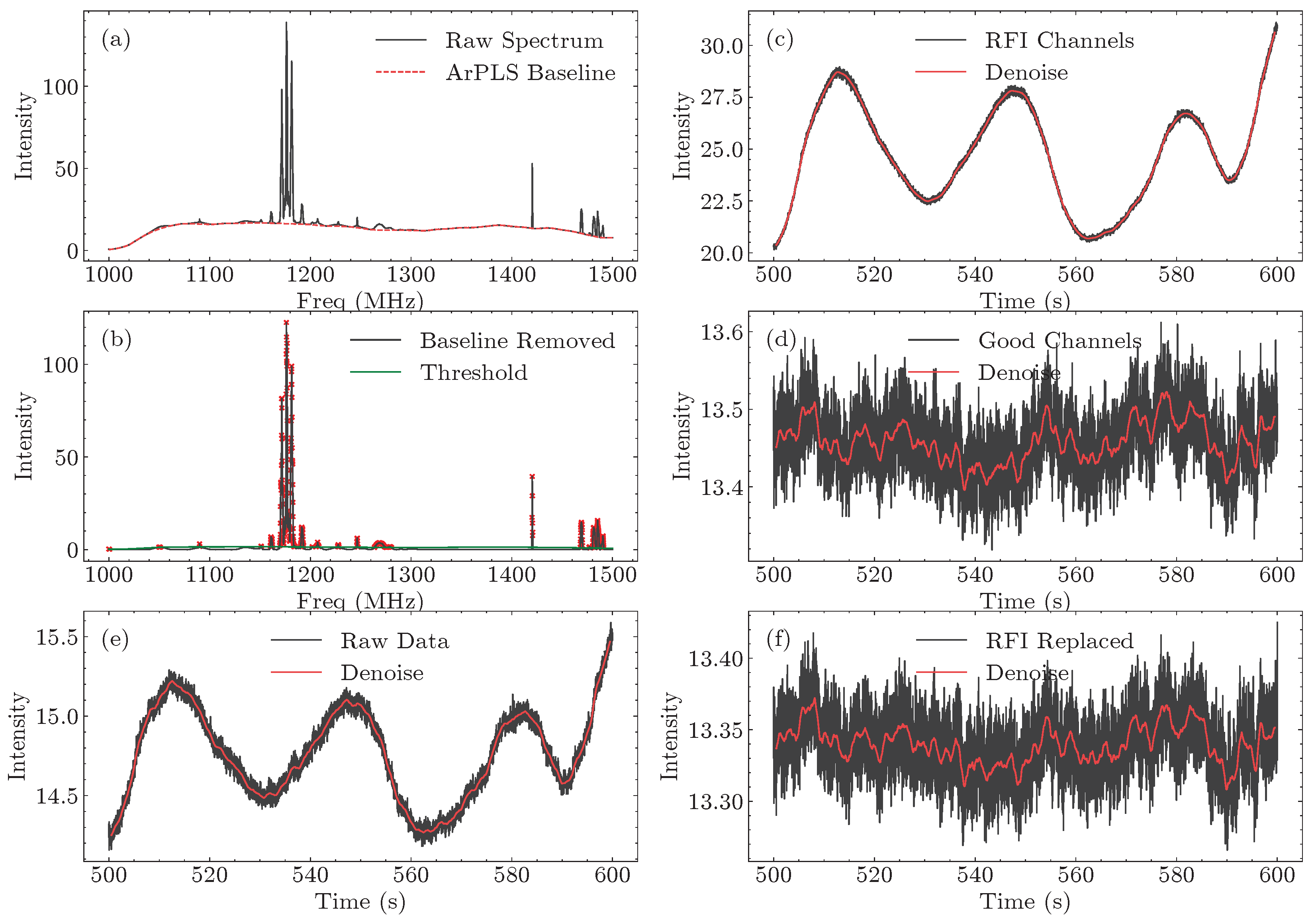
After extracting data from FITS files, we divide the observation into time segments of 10–100 s. The mean spectrum of each segment is used to estimate the baseline via ArPLS method. Once the baseline is subtracted, RFIs are flagged as channels exceeding n times the standard deviation baseline, as shown in the subplot (a) and (b) Figure 1. RFI channels are then replaced by baseline or set to zero. The light curve before and after the RFI mitigation is shown in the subplot (e) and (f) of Figure 1. Thus, in some cases, RFI signals are so strong that they can dominate the entire light curve, producing false signals.

2.3. Temperature

The raw data extracted from the FITS files are power data in the FAST signal receiver. To recover the corresponding antenna temperature and flux density, calibration using the injected noise is required. In the following, we refer to on-source and off-source data as “ON” and “OFF”, while data with noise diode switched on are prefixed with “CAL”.

We employ a simple Python 3.8.13-based method to separate the raw data with injected noise, $P_{CAL}$, from those without noise, P. The power is then converted to temperature as:

$$\begin{array}{c}\hfill T=({\displaystyle \frac{P_0}{P_{CAL0}-P_0}}{T}_{CAL0}+{\displaystyle \frac{P_1}{P_{CAL1}-P_1}}{T}_{CAL1})/2,\end{array}$$

(1)

where the subscripts 0 and 1 correspond to the two orthogonal receivers, and $T_{CAL}$ represents the noise diode temperature provided by the FAST calibration report.

After the temperature is recovered, the system temperature must be subtracted from the on-source temperature to obtain the source contribution. In tracking mode, the system temperature can only be derived through the fitted function of ZA as below:

$$\begin{array}{c}\hfill T_{sys}=P_0\times arctan(\sqrt{1+{{\theta }_{ZA}}^n}-P_1)+P_2,\end{array}$$

(2)

where $P_0$, $P_1$ and $P_2$ are fitting parameters from Jiang et al. [36], and ${\theta }_{ZA}$ is the zenith angle. When the ZA is smaller than 10°, the system temperature increases by up to 1 K and reaches its minimum in the range of $[10°,15°]$. When the ZA is greater than $15$, it can vary by 5–7 K. In an observation with length of ∼1000 s, $T_{sys}$ can vary by 1–2 K, which is the main limitation in long-term calibration of FAST.

In On–Off mode observations, we also need to consider whether the off source is truly a cold sky. When using tracking mode or when the off-source position is not a completely cold sky, we apply the standard Equation (2) to calculate system temperature. Otherwise, we use off-source data to calculate the system temperature. The system temperature $T_{sys}$ and source temperature $T_{src}$ are then obtained through:

$$\begin{array}{ccc}\hfill T_{src}& =& T_{ON}-T_{sys}\hfill \\ & =& T_{ON}-T_{OFF},\hfill \end{array}$$

(3)

where $T_{ON}$ and $T_{OFF}$ are calculated from Equation (1) using on-source and off-source data.

Once $T_{src}$ is obtained, the corresponding flux density $S_{src}$ can be calculated by dividing by the gain G as:

$$\begin{array}{c}\hfill S_{src}={\displaystyle \frac{T_{src}}{G}}.\end{array}$$

(4)

The full and effective gains of FAST are expressed as $G_0=A_{geo}/2k,G=A_{eff}/2k$, where $A_{geo}$ and $A_{eff}$ are the geometric and effective illumination areas, respectively. The full gain $G_0$ of FAST is 25.6 K · Jy⁻¹. Aperture efficiency $\eta$ can be calculated from:

$$\begin{array}{c}\hfill \eta =\left\{\begin{array}{cc}a{\theta }_{ZA}+b,\hfill & 0°\le {\theta }_{ZA}\le 26.4°\hfill \\ c{\theta }_{ZA}+d,\hfill & 26.4°<{\theta }_{ZA}\le 40°,\hfill \end{array}\right.\end{array}$$

(5)

where a, b, c and d are fitted parameters from Jiang et al. [36].

In our observations, we observed the calibration source 3C 286 on the same day as the microquasar observations using On–Off mode to obtain absolute gain [40]. Using the same procedures mentioned above, the absolute gain can be calculated as:

$$\begin{array}{ccc}\hfill log\left(S_{3C286}\left(f\right)\right)& =& 1.2481-0.4507log\left(f\right)\hfill \\ & & -0.1798{log}^2\left(f\right)+0.0357{log}^3\left(f\right)\hfill \end{array}$$

(6)

$$\begin{array}{ccc}\hfill G_{3C286}& =& T_{3C286}/S_{3C286},\hfill \end{array}$$

(7)

where f is the frequency, and $T_{3C286}$, $S_{3C286}$ and $G_{3C286}$ represent the temperature of 3C 286 calculated using Equation (3), the standard flux density of 3C 286 and the derived absolute gain. The spectral index can then be derived from $S\left(\nu \right)\propto {\nu }^{\alpha },\alpha =\Delta logS\left(\nu \right)/\Delta log\nu .$

2.4. Polarization Calibration

The polarization calibration follows a single-axis pipeline that assumes perfectly orthogonal receptors with equal intensity and phase response, which is the noise injection here. The FAST is equipped with a full-polarization receiver system that measures four polarization components, XX, YY, CR, and CI, corresponding to the two orthogonal linear polarization intensities and the real and imaginary parts of the cross-correlation between X and Y directions. From these components, the four Stokes parameters (I, Q, U, V) can be derived as follows:

$$\begin{array}{c}\hfill I=XX+YY={E_x}^2+{E_y}^2\\ \hfill Q=XX-YY={E_x}^2-{E_y}^2\\ \hfill U=2·CR=2Re(E_x·E_y)\\ \hfill V=2·CI=2Im(E_x·E_y),\end{array}$$

(8)

where $E_x$ and $E_y$ denote the complex electric field voltages in X and Y directions. Considering that the feed system is not perfect, there inevitably exist phase and gain differences between two orthogonal directions. Using the noise intensity of four polarization channels can greatly correct for the deviations.

Three parameters are defined for correction: phase delay Chi $\chi$, leakage $f_{leak}$ and normalization factor $G_{norm}$. The phase delay between $I_x$ and $I_y$ is represented by $\chi$. Gain differences between orthogonal receivers are quantified as leakage between Stokes parameters I and Q, while gain is a factor that normalizes Stokes parameters. We define the Stokes parameters of noise signals as:

$$\begin{array}{cc}& CALI=(CALXX-XX)+(CALYY-YY)\\ & CALQ=(CALXX-XX)-(CALYY-YY)\\ & CALU=2·(CALCR-CR)\\ & CALV=2·(CALCI-CI).\end{array}$$

(9)

We can then derive leakage, delay and gain as:

$$\begin{array}{cc}& f_{leak}={\displaystyle \frac{CALQ}{CALI}}\\ & \chi ={\displaystyle \frac{1}{2}}arctan{\displaystyle \frac{CALV}{CALU}}\\ & CAL{U}_{true}=CALU·cos\left(\chi \right)+CALV·sin\left(\chi \right)\\ & CAL{I}_{true}=(CALI-f_{leak}·CALQ)/(1-f_{leak}^2)\\ & G_{norm}=CALI,\end{array}$$

(10)

$f_{leak}$, $\chi$ and $G_{norm}$ represent the calibration parameters leakage, delay and normalization factor. $CAL{I}_{true}$ and $CAL{U}_{true}$ are corrected noise Stokes parameters.

After the calibration parameters are obtained, we can now calculate the corrected Stokes parameters as:

$$\begin{array}{cc}& I_{\mathrm{true}}=\left({\displaystyle \frac{I_{\mathrm{obs}}-f_{leak}·Q_{\mathrm{obs}}}{1-f_{leak}^2}}\right)/G_{norm}\\ & Q_{\mathrm{true}}=\left({\displaystyle \frac{Q_{\mathrm{obs}}-f_{leak}·I_{\mathrm{obs}}}{1-f_{leak}^2}}\right)/G_{norm}\\ & U_{\mathrm{true}}=(U_{\mathrm{obs}}cos\chi +V_{\mathrm{obs}}sin\chi )/G_{norm}\\ & V_{\mathrm{true}}=(V_{\mathrm{obs}}cos\chi -U_{\mathrm{obs}}sin\chi )/G_{norm}\\ & L=\sqrt{{Q_{true}}^2+{U_{true}}^2}\\ & P=\sqrt{L^2+{V_{true}}^2}.\end{array}$$

(11)

where L and P represent the linear polarization intensity and total polarization intensity. Stokes parameters with subscript “obs” and “true” represent the observed Stokes parameters and the corrected ones, respectively.

Finally, the linear polarization degree (LP), circular polarization degree (CP) and polarization angle (PA) can be calculated as:

$$\begin{array}{cc}& LP={\displaystyle \frac{L}{I_{true}}}\\ & CP={\displaystyle \frac{V_{true}}{I_{true}}}\\ & PA={\displaystyle \frac{1}{2}}arctan{\displaystyle \frac{U_{true}}{-Q_{true}}}.\end{array}$$

(12)

We note that, in the case of the FAST, the Stokes parameter –Q should be used when calculating the PA in order to be consistent with the International Astronomical Union (IAU) definition.

It should be pointed out that the lower linear polarization degree or the lower the source intensity is relative to random noises intensity, the higher the impact of random noise on the estimated LP. As Equation (12) puts it, the LP is calculated as L/P, where L is given by $L=\sqrt{Q_{true}^2+U_{true}^2}$. Thus, random noise will be accumulated, and the LP will be overestimated. The LP will appear to fluctuate around a value that is much larger than the real value, and thus, calculating the mean value of the LP over time will give an overestimated value. In addition, the PA will also be affected due to its arctan relation of Q and U. The CP stays the same because its calculation contains no non-linear functions so that taking the average before or after will not make any difference.

This issue is widely discussed in studies on pulsars and fast radio bursts (FRBs). FRBs and single pulses are short-duration events where the LP and PA changes rapidly, making it impossible to rule out the effect of random noise by taking the average in the time domain. Everett and Weisberg [41] proposed a method of calculating the unbiased linear polarization intensity $L_{debiased}$ using the measured $L_{bias}$ and the standard deviation of Stokes I $sigm{a}_I$ as:

$$\begin{array}{c}\hfill L_{debiased}=\left\{\begin{array}{cc}\sqrt{{\left({\displaystyle \frac{L_{bias}}{{\sigma }_I}}\right)}^2-1{\sigma }_I}\hfill & if{\displaystyle \frac{L}{{\sigma }_I}}\ge 1.57.\hfill \\ 0\hfill & otherwise.\hfill \end{array}\right.\end{array}$$

(13)

In cases of microquasars, we assume that the LP and PA evolve much more slowly than the timescale of random noise. Therefore, polarization calibration can be improved by averaging Stokes parameters over timescales of 0.1–1 s to effectively suppress random noise. Subtracting the averaged background gives the real value of them. Applying Equation (12) after that will give accurate polarization results. This does not mean that polarization information is lost during the polarization calibration; fast variations of polarization are still reliable.

3. Results

3.1. Temperature and Flux Density

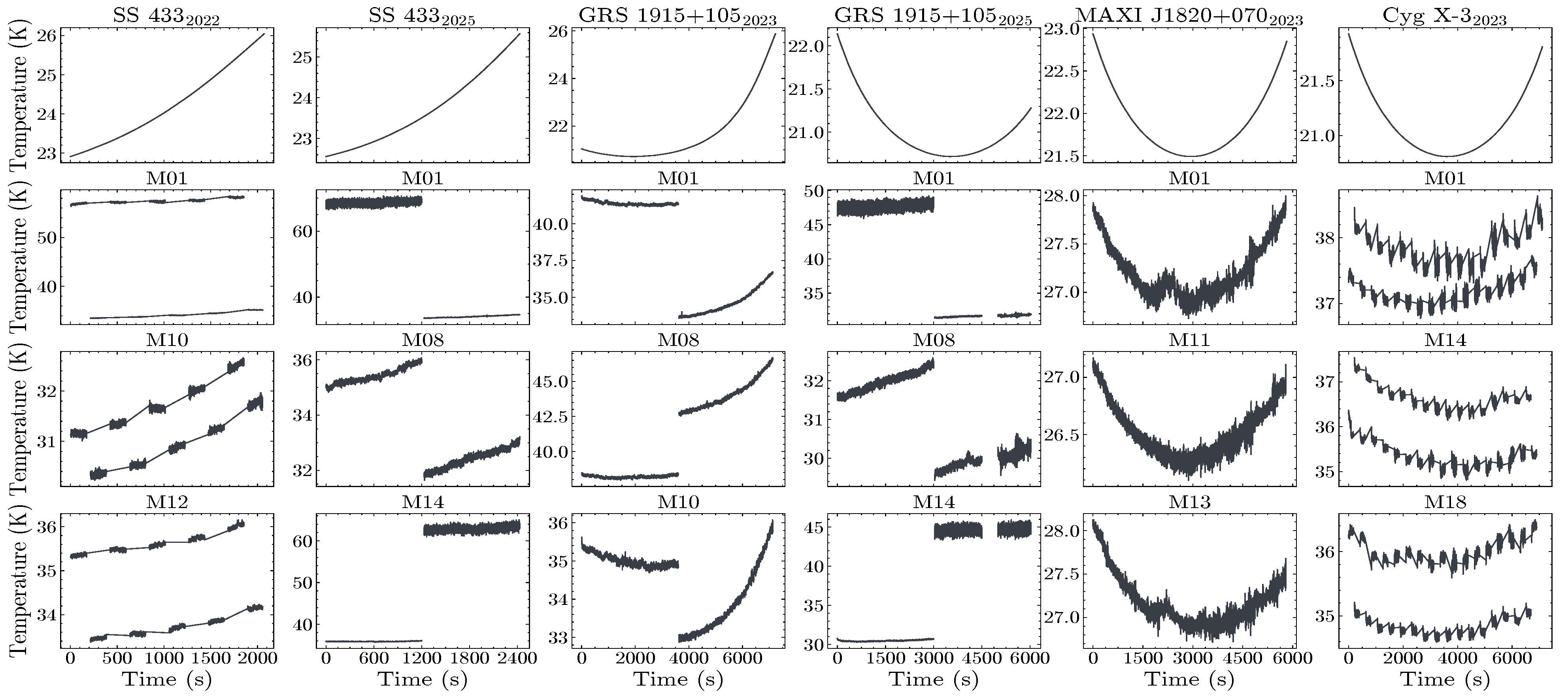
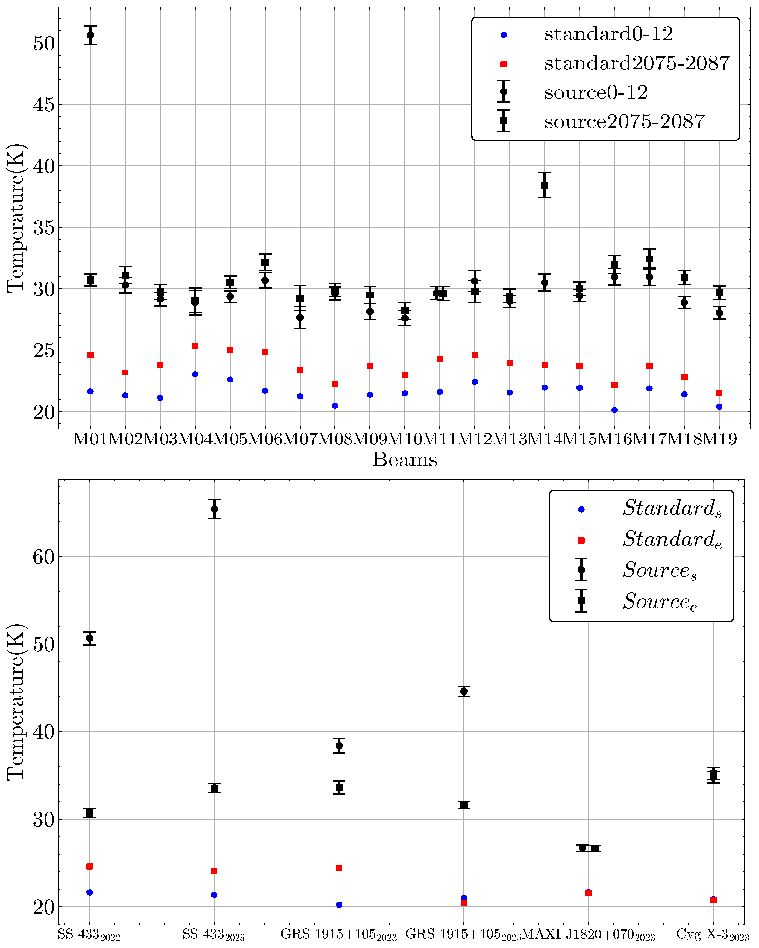
Firstly, after extracting the raw data and separating the noise data, temperature curves were reconstructed. In Figure 2, we calculate the temperatures of these observations using the same frequency channels between 1317 MHz and 1415 MHz, where RFI is minimal. The multi-beam temperature curves of these sources along with system temperature are shown in Figure 3. The temperature curve of each source exhibits a trend that is generally consistent with the fitted $T_{sys}$. Nevertheless, we note that variations caused by system temperature can never be completely removed, which is also the reason why we present the calibration results only for the time segments closest to the reliable background, rather than the entire curves.

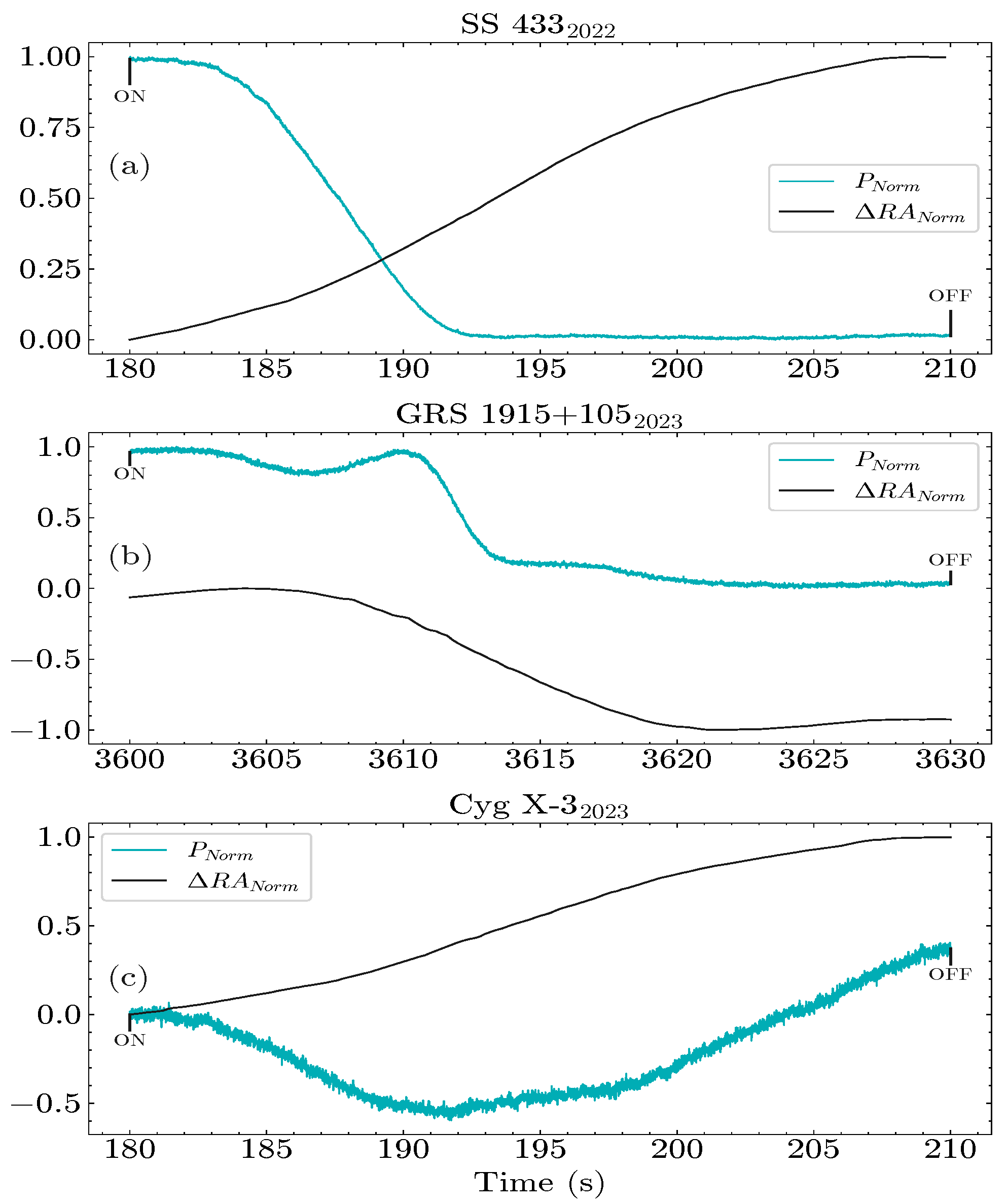
For On–Off observations, the power curves during On–Off switching along with the Right Ascension (RA) curves are shown in Figure 4. Gain will change naturally as the beam center moves away from the source, leading to a decrease in the received power. In all observations presented in this paper, the beams were moved along a constant Declination (Dec) to change the RA, so the RA offset $\Delta RA=RA-RAsrc$ represents the distance of the central beam from the source. The black curve and blue curve in this Figure are normalized RA offset and flux density curve, respectively. As shown in Figure 4, the power of SS 433 and GRS 1915+105 keeps falling to a value and stays there as the RA keeps changing. Thus, we can say that SS 433 and GRS 1915+105 have radio emission and a clear off-source background. For Cyg X-3, the power decreases to a minimum point and increases to a value even greater than the on-source power, indicating that the off-source position is contaminated by some other radio source.

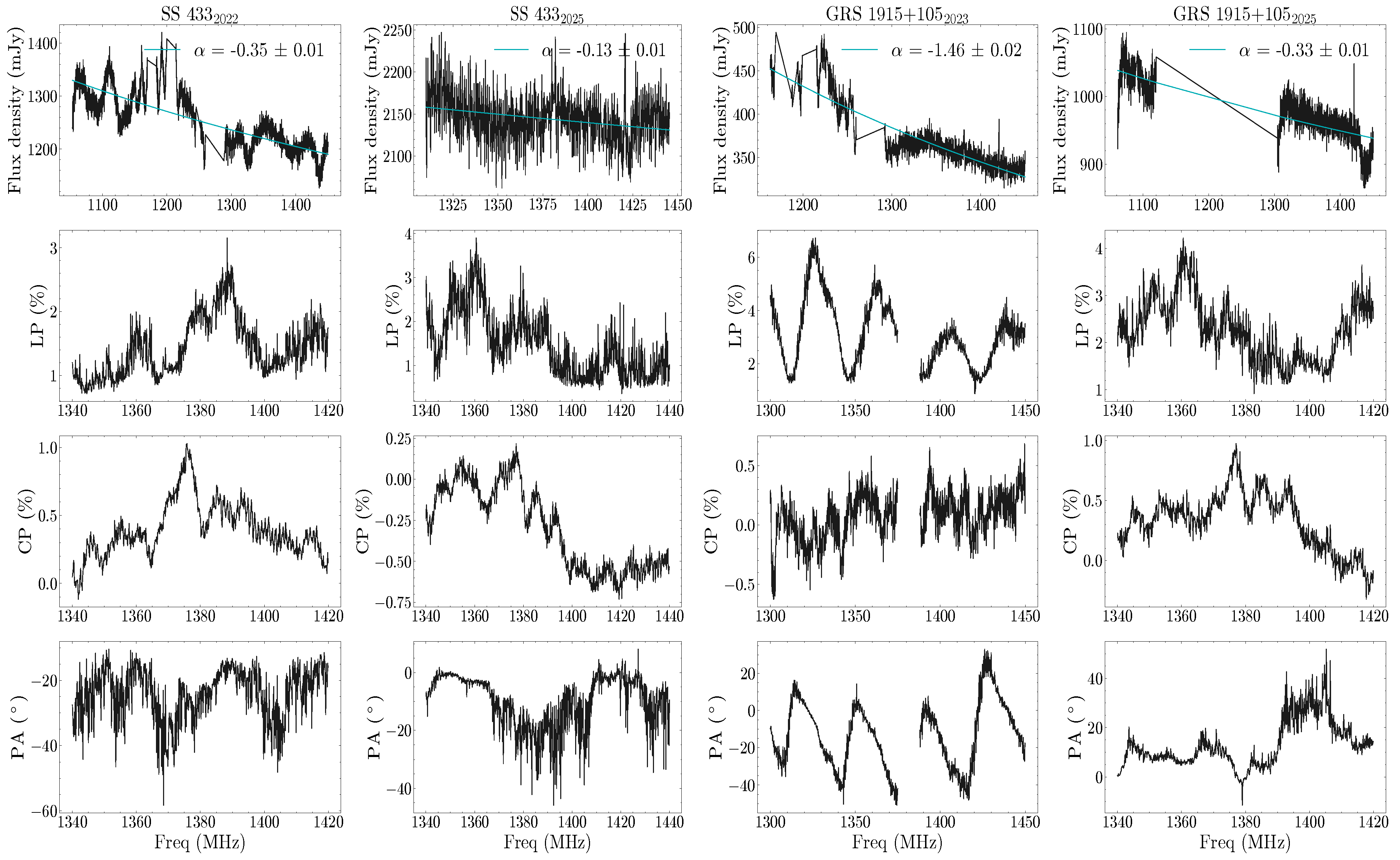
For SS 433 and GRS 1915+105, we present the absolute flux densities and polarization results calibrated from the clearest and most reliable off-source backgrounds in Table 2. For Cyg X-3 and MAXI J1820+070, where $T_{sys}$ could not be obtained from observations, we used the system temperature model to calculate the flux density and spectral index. The polarization results could not be obtained due to the lack of background.

Table 2. Flux density and polarization parameters for the microquasars in six observations.

Source Name	UTC	Flux Density a (Jy)	Spectral Index	LP (%)	CP (%)	PA (°)
SS 433	21 October 2022 10:35:27	1.20	−0.35 ± 0.01	1.43	0.40	−24.25
	6 January 2025 05:21:00	2.09	−0.13 ± 0.01	1.49	−0.30	−9.99
GRS 1915+105	6 September 2023 12:35:00	0.34	−1.46 ± 0.02	3.10	0.07	−13.11
	27 January 2025 02:43:00	0.94	−0.33 ± 0.01	2.27	0.33	13.10
Cyg X-3	7 January 2023 05:19:00	0.80	−1.73 ± 0.01	-	-	-
MAXI J1820+070	12 September 2023 11:00:00	0.32	−1.45 ± 0.02	-	-	-

^a Flux density shown here represents the flux density at 1.45 GHz. LP, CP and PA are calculated by taking mean values over good channels shown in Figure 5.

Table 2. Flux density and polarization parameters for the microquasars in six observations.

Source Name	UTC	Flux Density a (Jy)	Spectral Index	LP (%)	CP (%)	PA (°)
SS 433	21 October 2022 10:35:27	1.20	−0.35 ± 0.01	1.43	0.40	−24.25
	6 January 2025 05:21:00	2.09	−0.13 ± 0.01	1.49	−0.30	−9.99
GRS 1915+105	6 September 2023 12:35:00	0.34	−1.46 ± 0.02	3.10	0.07	−13.11
	27 January 2025 02:43:00	0.94	−0.33 ± 0.01	2.27	0.33	13.10
Cyg X-3	7 January 2023 05:19:00	0.80	−1.73 ± 0.01	-	-	-
MAXI J1820+070	12 September 2023 11:00:00	0.32	−1.45 ± 0.02	-	-	-

^a Flux density shown here represents the flux density at 1.45 GHz. LP, CP and PA are calculated by taking mean values over good channels shown in Figure 5.

Figure 5. Calibration results. From top to bottom: flux density, LP, CP, PA. Blue line in the top panel represents the fitted spectral index line.

Figure 5. Calibration results. From top to bottom: flux density, LP, CP, PA. Blue line in the top panel represents the fitted spectral index line.

3.2. Polarization

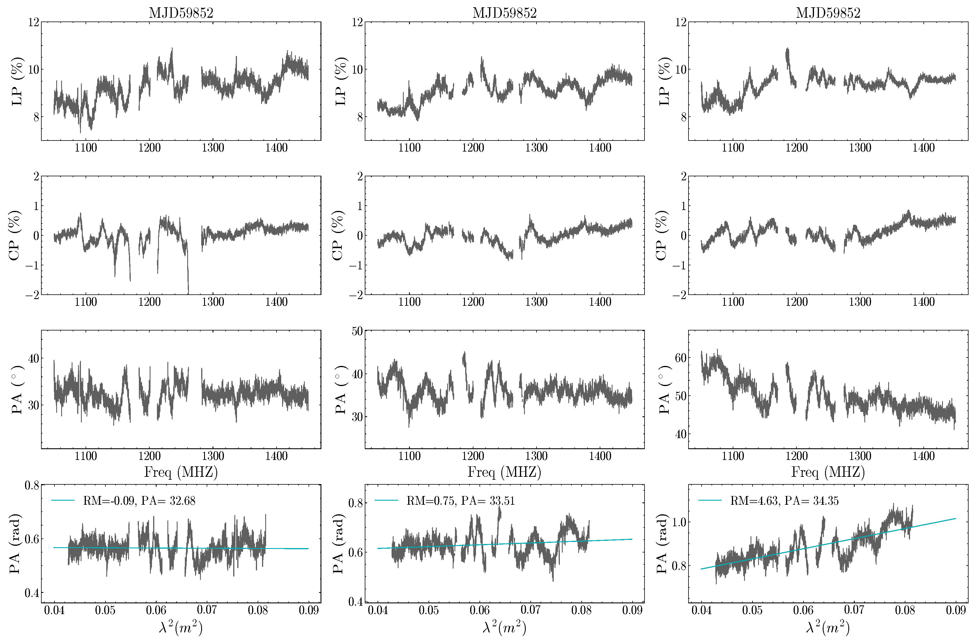
In our observations, 3C 286 was observed multiple times to calibrate the absolute gain of FAST. Therefore, we adopted the polarization calibration method mentioned in Section 2.4 to validate our polarization calibration procedures. Each observation of 3C 286 recorded 60 s of on-source and 60 s of off-source, with 30 s of switching between them. Three sets of 3C 286 observations are shown in Figure 6. The rotation measure (RM) and PA are calculated by fitting the PA curve with a linear function $P{A}_f=P{A}_{\infty }+RM·{\lambda }^2$. Errors are within acceptable range considering unavoidable interference. The LP and PA are in agreement with the standard polarization derived previously [42].

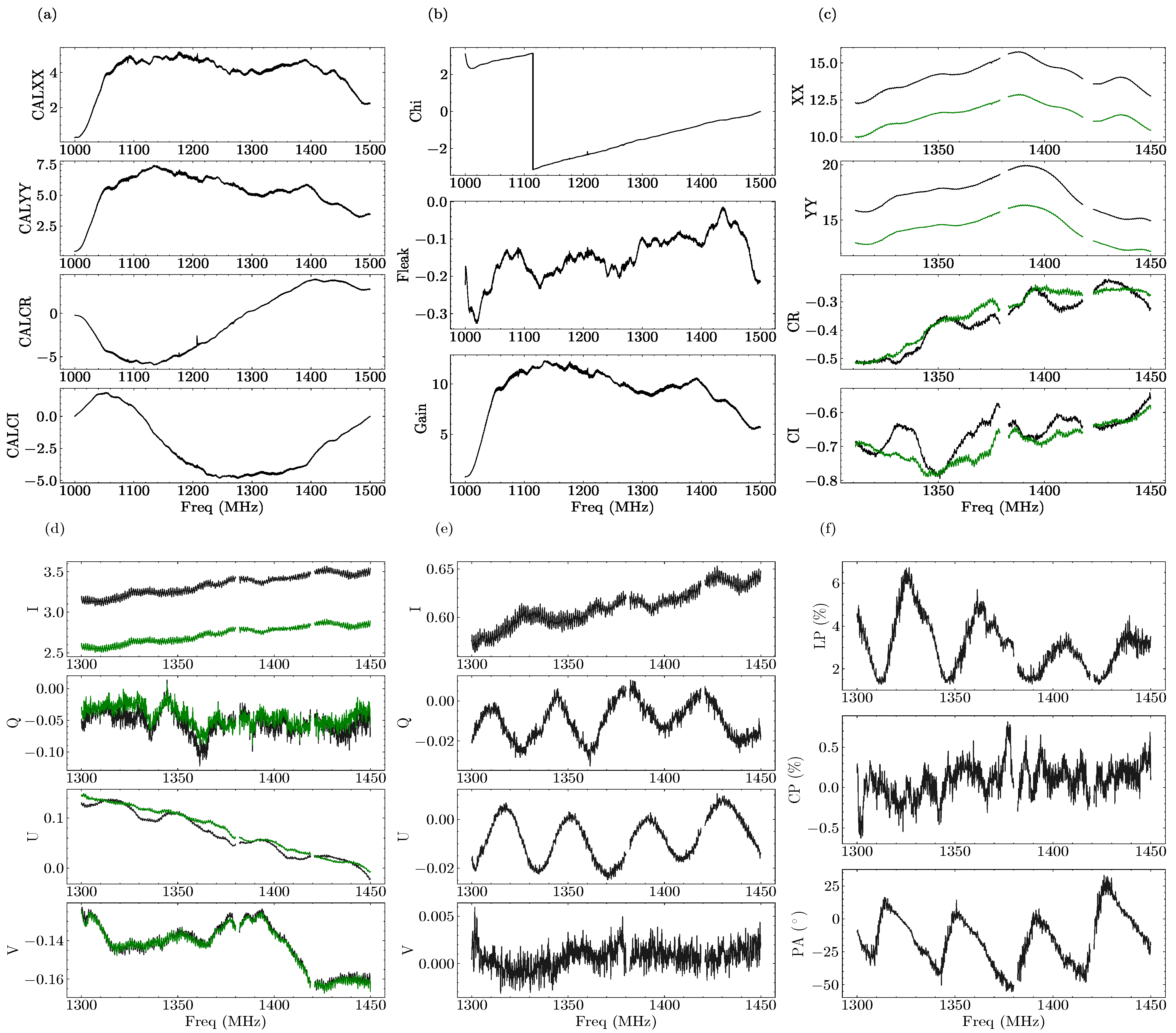
We adopted this polarization calibration pipeline on our observations. Similar to the varying the system temperature, the background Stokes parameters are also changing throughout observations. Therefore, we present the polarization calculated with the best background in Table 2 and show the detailed results in Figure 5. A sample of the calibration procedures is shown in Figure 7.

4. Discussion

4.1. Variation Quantification

To verify the presence of celestial emission and to quantify the source activity, we introduce the cross-correlation analysis among the 19-beam data from FAST. For On–Off observations, the existence of celestial radiation can be directly inferred from the power variation during On–Off switching, as shown in Figure 4. If the power decrease can be ignored within the noise level, the source flux density can be regarded as undetectable. For tracking observations, we can still quantify the source activity and independence among 19 beams by calculating cross-correlation coefficients between them.

To quantify correlation and independence, we adopt both the Pearson correlation coefficient (PCC) method and the distance correlation (dCor) method. The results of both methods range from 0 to 1, with larger values indicating stronger correlations. These two methods are straightforward to interpret, capable of capturing both linear and non-linear correlations, and computationally efficient.

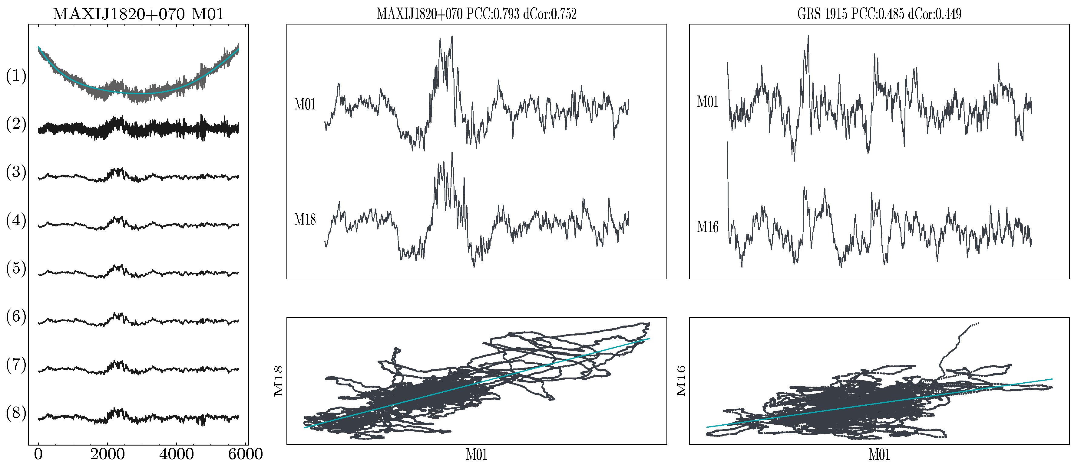
Before computing correlations, long-term trends caused by ZA variations during source tracking are removed using polynomial fitting of order 5 and carefully checked in case of overfitting. Furthermore, random noise is suppressed using multiple denoising methods, including Fast Fourier Transform (FFT), median, sliding window, Empirical Mode Decomposition (EMD), Gaussian, and ArPLS filtering. An example of this detrending and denoising processes applied to MAXI J1820+070 is shown in Figure 8.

In MAXI J1820+070, we observed a peak structure around 2000 s. Considering that the temperature of M01 is not higher than that of the other beams and only slightly exceeds the system temperature calculated from Equation (2), its authenticity needs to be verified. In Figure 3, peaks are also found in other beams at approximately the same time. As shown in Figure 8, M01 and M18 exhibit highly correlated variations. The PCC value of ∼0.79 indicates that light curves of different beams are highly correlated. We therefore conclude that no significant radio radiation from MAXI J1820+070 was detected and that its temperature curve was dominated by red noise.

Similar analyses were performed on other sources. We also show the result of 2023 observation on GRS 1915+105 in Figure 8. By comparing the temperature curves of M01 and M14 for GRS 1915+105, we find that segments with large fluctuations occur simultaneously in these beams, suggesting that these fluctuations are most likely due to variations in system temperature or noise. The PCC and dCor results of ∼0.48 and 0.45 also suggest remarkable correlation. A short continuous on-source duration of 180 s reduced the influence of red noise in SS 433 and Cyg X-3. In the 2025 observations, SS 433 and GRS 1915+105 showed high flux densities with stable light curves (Figure 3).

In summary, no significant radiation was detected in MAXI J1820+070. SS 433, GRS 1915+105 and Cyg X-3 showed flux densities that can be attributed to intrinsic source activity. We suggest that in long-duration continuous observations, careful inspection should be performed among multiple beams to rule out the effect of system temperature and red noise in future radio observations.

4.2. Flux Density and Polarization

The flux density and polarization results are presented in Figure 5 with good channels. The high flux densities suggest that SS 433 and GRS 1915+105 both underwent radio flares in early 2025 [43]. In terms of polarization, microquasars generally exhibit low LP and CP values. The low LP, intensity fluctuations around certain frequencies and superposition of multiple jet components can lead to great uncertainty in calculating the PA, as shown in the fourth panel of this figure.

Specially, during the 2023 observation on GRS 1915+105, clear oscillation of the LP and PA on frequency was recorded. As shown in the calibration procedure (Figure 7), the oscillation of Stokes Q and U is the direct cause of the polarization oscillation. The oscillation in the circular polarization degree cannot be clearly recognized. This oscillation may indicate the existence of Faraday conversion or frequency-dependent absorption. This phenomenon most likely originates from the magnetic field near the donor star. Moreover, after years of outbursts, GRS 1915+105 entered an obscured phase in 2019 and underwent several X-ray flares [44]. Our radio observation in 2023 was performed near the flare 3 and showed an optically thin spectrum, indicating that the emissions may originate from transient jets during a state transition [44].

4.3. QPOs

In general, X-ray QPOs have been widely detected across different accreting systems and accretion states, spanning a wide range of periods and behaviors. For GRS 1915+105, periods of tens of minutes are observed not only in the X-ray band [45] but also in the radio and infrared bands [7,46]. These variations can be well explained by the periodic disappearance and replenishment of the inner 200 km of the accretion disk and indicate a strong, non-linear correlation between the accretion and jet formation [47,48,49,50]. However, rapid X-ray variations, such as the 67 Hz QPO that is thought to be related to the Keplerian period of the innermost stable orbit, are rarely detected at other wavelengths [6,50]. The low-frequency QPOs from ∼0.1–10 Hz are observed in most black hole X-ray transients [51,52,53]; however, the physical origin is still unclear [10]. The transient and weak radio QPOs around 5 Hz reported by FAST firstly were the first to connect the QPO production to dynamics of relativistic jets of the microquasar [9]. The transient GHz band polarization oscillations at 17 and 33 s in GRS 1915+105 show the first evidence for the polarization QPOs in black hole systems [8], which would be interesting for understanding magnetic field configuration near the black hole.

Here, considering the fast radio variations in microquasars, we tried to search for the possible QPOs using the FAST. To perform periodicity analysis, we applied FFT and wavelet transforms on the flux density curve derived in Section 3.1. Multiple artificial and instrumental effects can cause false periodic signals.

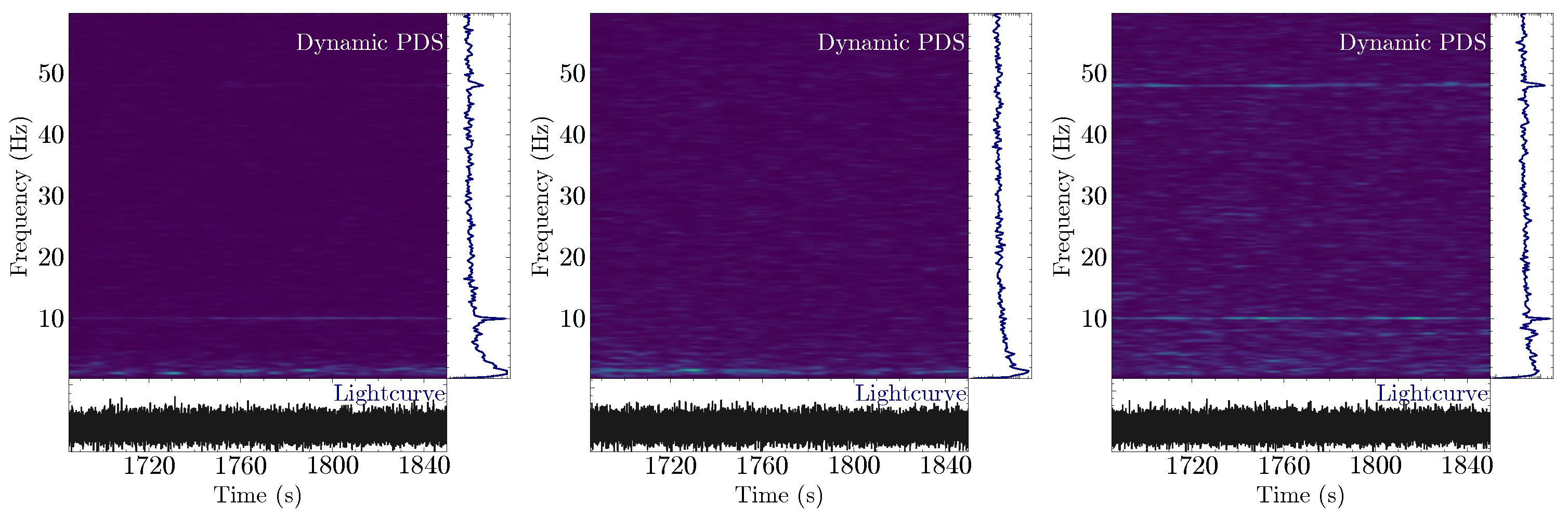
In the high-frequency domain, high-frequency noise is generally observed in radio observations. Noise components of 47Hz, 50 Hz, 53.5 Hz and 10 Hz are the most commonly recorded artificial signals. As shown in Figure 9, signals of 10 Hz and 50 Hz appeared in both M01 and M19 but were not recorded in M10. Detailed inspections on multi-beams and polarization channels are required to prove the authenticity of detected signals.

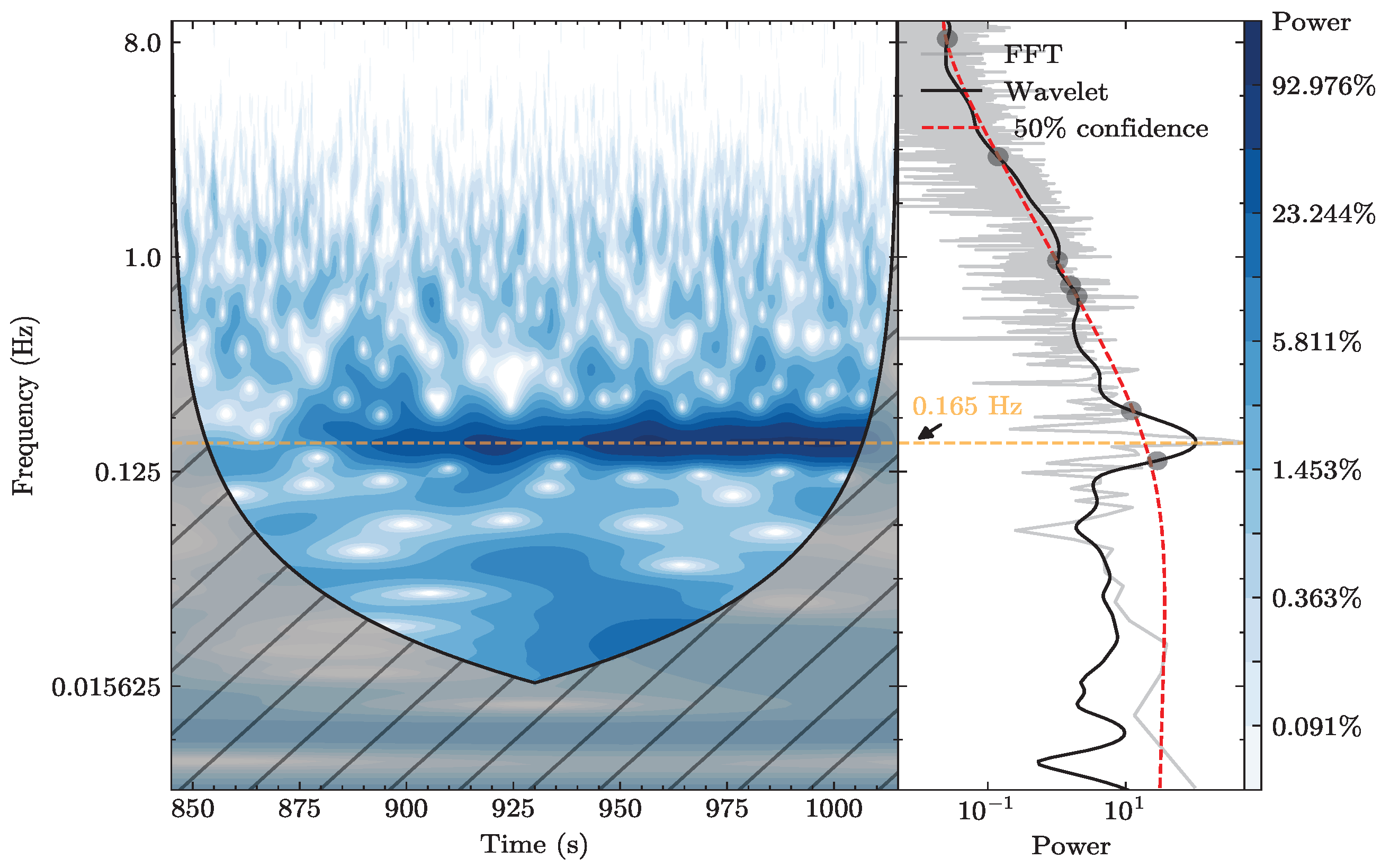
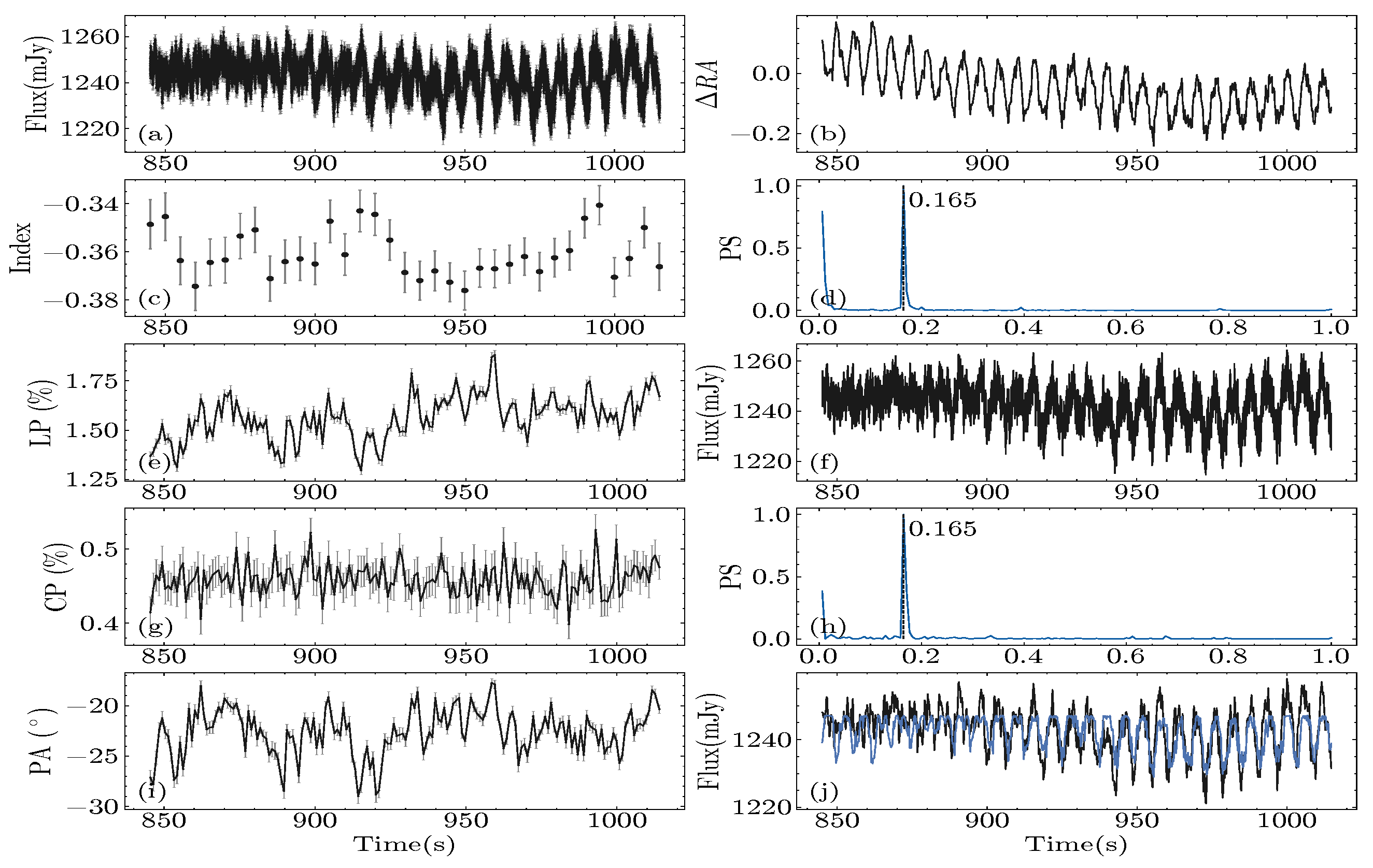
In the low-frequency domain, apparent periodic oscillations mainly come from feed oscillations. After position switching, the FAST feed may oscillate at a period of several seconds, causing fake signals. These oscillations are typically observed only in the central beam M01, as gain fluctuations caused by pointing offset can affect the measured flux density only in the presence of a radio-emitting source within the beam. An example is shown in Figure 10. The period of ∼6 s can be clearly identified in both the flux density and RA offset curve between 900 and 1015 s, and their power spectra both show a peak at 0.165 Hz. We fitted the flux density S with Gaussian model $S=a+b·exp\left({\displaystyle \frac{-{\Delta RA}^2}{2c^2}}\right)Jy$ on RA offset in subplot (j), where a, b and c are free parameters. A clear Gaussian relationship can be fitted, but it should be noted that no method can precisely eliminate the effect of feed oscillations to date.

After careful inspection, we failed to detect any credible radio QPOs from 0.01–100 Hz with the present FAST observations. The previous report on the QPOs in GRS 1915+105 showed the strong correlation with the increase in flux density and high activity. Overall, as we discussed in the previous sections, the microquasars exhibited low activity throughout our hour-long observations in this work. The absence of radio QPOs may be attributed to the stable state of these systems. On the other hand, whether the jet originates from the inner disk or the corona remains an important issue [54,55]. The region that leads to X-ray QPOs may not be directly connected to the injection of ejecta, which could explain the lack of corresponding radio counterparts. The connection between the X-ray QPOs and radio QPOs requires further simultaneous observations on these microquasars in both X-ray and radio bands.

5. Conclusions

In this work, we have established a standard calibration pipeline for FAST observations of microquasars, which is important for the near-future FAST monitoring on all microquasars in the northern sky. Before the observation, careful inspection of the surrounding radio environment is necessary to select a cold off-source area for system temperature and background Stokes parameters. The intensity variations during position switching can serve as an indicator of the existence of source radiations. User-defined noise should also be chosen based on the observation goals. Fast noise injection not only improves temperature calibration precision but also preserves the intrinsic variations of the source. ArPLS is then employed to obtain the spectral baseline, which is then used to identify and mitigate RFI channels. Noise injection ensures subsequent calibration of temperature and polarization.

In the early stages of our microquasar observations, we observed four sources. GRS 1915+105, SS 433 and Cyg X-3 were clearly detected, while cross-beam correlation analysis indicated that MAXI J1820+070 showed no significant radio activity. Both GRS 1915+105 and SS 433 exhibited low linear polarization fractions of several percent, consistent with previous works and indicating that the jet magnetic field is relatively disordered [56,57]. We also recorded oscillations of polarization on frequency in GRS 1915+105, which is thought to be related to the Faraday conversion by magnetic field of the companion star. We searched for the possible radio QPOs with the frequencies from 0.01 to 100 Hz in six observations, and no credible signals were confirmed.

In the future, we plan to conduct more simultaneous multi-wavelength observations, including the highly sensitive FAST observations, which are particularly suitable for detecting subtle and rapid variations. A primary goal of upcoming works will be to determine whether radio QPOs are universal or occur only during specific accretion states. Coordinated X-ray observations will play an essential role in identifying the accretion state of microquasars. Simultaneous radio monitoring may reveal whether radio QPOs share temporal or frequency correlations with X-ray counterparts. Establishing such connections would lead to a decisive step toward uncovering the physical origin of QPOs and the link between accretion dynamics and jet generation.

References

1. Mirabel, I.F.; Rodriguez, L.F. Sources of relativistic jets in the galaxy. Annu. Rev. Astron. Astrophys. 1999, 37, 409–443. [Google Scholar] [CrossRef]
2. Fender, R.P. Powerful jets from black hole X-ray binaries in low/hard X-ray states. Mon. Not. R. Astron. Soc. 2001, 322, 31–42. [Google Scholar] [CrossRef]
3. Fender, R.P.; Belloni, T.M.; Gallo, E. Towards a unified model for black hole X-ray binary jets. Mon. Not. R. Astron. Soc. 2004, 355, 1105–1118. [Google Scholar] [CrossRef]
4. Rodriguez, L.F.; Mirabel, I.F. An Unusual Change in the Radio Jets of GRS 1915+ 105. Astrophys. J. 2025, 986, 108. [Google Scholar] [CrossRef]
5. Rodríguez, L.F.; Mirabel, I.F. Fast sinusoidal oscillations in the radio flux of GRS 1915+ 105. Astrophys. J. 1997, 474, L123. [Google Scholar] [CrossRef]
6. Morgan, E.; Remillard, R.; Greiner, J. RXTE observations of QPOs in the black hole candidate GRS 1915+ 105. Astrophys. J. 1997, 482, 993. [Google Scholar]
7. Fender, R.P.; Pooley, G.G.; Brocksopp, C.; Newell, S. Rapid infrared flares in GRS 1915+ 105: Evidence for infrared synchrotron emission. Mon. Not. R. Astron. Soc. 1997, 290, L65–L69. [Google Scholar] [CrossRef]
8. Wang, W.; Chen, J.; Tian, P.; Ho, L.C.; Sun, X.; Wang, P.; Zhang, B.; Zheng, Z.; Chen, X.; Zhang, P.; et al. Quasi-periodic oscillations of GHz-band polarization in a black hole. Nat. Commun. 2025, 16, 5139. [Google Scholar] [CrossRef]
9. Tian, P.; Zhang, P.; Wang, W.; Wang, P.; Sun, X.; Liu, J.; Zhang, B.; Dai, Z.; Yuan, F.; Zhang, S.; et al. Subsecond periodic radio oscillations in a microquasar. Nature 2023, 621, 271–275. [Google Scholar] [CrossRef]
10. Wang, W. Observations of Fast Radio Variations in Microquasars by FAST. Chin. Phys. Lett. 2024, 41, 119701. [Google Scholar] [CrossRef]
11. Blundell, K.M.; Bowler, M.G. Symmetry in the changing jets of SS 433 and its true distance from us. Astrophys. J. 2004, 616, L159. [Google Scholar] [CrossRef]
12. Cherepashchuk, A.; Sunyaev, R.; Fabrika, S.; Postnov, K.; Molkov, S.; Barsukova, E.; Antokhina, E.; Irsmambetova, T.; Panchenko, I.; Seifina, E.; et al. INTEGRAL observations of SS433: Results of a coordinated campaign. Astron. Astrophys. 2005, 437, 561–573. [Google Scholar] [CrossRef]
13. Cherepashchuk, A.; Postnov, K.; Molkov, S.; Antokhina, E.; Belinski, A. SS433: A massive X-ray binary in an advanced evolutionary stage. New Astron. Rev. 2020, 89, 101542. [Google Scholar] [CrossRef]
14. Stephenson, C.; Sanduleak, N. New H-alpha emission stars in the Milky Way. Astrophys. J. Suppl. Ser. 1977, 33, 459–469. [Google Scholar] [CrossRef]
15. Margon, B.; Ford, H.; Katz, J.; Kwitter, K.; Ulrich, R.; Stone, R.; Klemola, A. The bizarre spectrum of SS 433. Astrophys. J. Part 2-Lett. Ed. 1979, 230, L41–L45. [Google Scholar] [CrossRef]
16. Margon, B.; Ford, H.C.; Grandi, S.A.; Stone, R.P. Enormous periodic Doppler shifts in SS 433. Astrophys. J. Part 2-Lett. Ed. 1979, 233, L63–L68. [Google Scholar] [CrossRef]
17. Liebert, J.; Angel, J.; Hege, E.; Martin, P.; Blair, W. The moving emission features in SS433 require a dynamical interpretation. Nature 1979, 279, 384–387. [Google Scholar] [CrossRef] [PubMed]
18. Cherepashchuk, A. Observational manifestations of precession of accretion disk in the SS 433 binary system. Space Sci. Rev. 2002, 102, 23–35. [Google Scholar] [CrossRef]
19. ABELL, G.O.; MARGON, B. A kinematic model for SS433. Nature 1979, 279, 701–703. [Google Scholar] [CrossRef]
20. Castro-Tirado, A.; Brandt, S.; Lund, N. GRS 1915+ 105. Int. Astron. Union Circ. 1992, 5590, 2. [Google Scholar]
21. Reid, M.; McClintock, J.; Steiner, J.; Steeghs, D.; Remillard, R.; Dhawan, V.; Narayan, R. A parallax distance to the microquasar GRS 1915+ 105 and a revised estimate of its black hole mass. Astrophys. J. 2014, 796, 2. [Google Scholar] [CrossRef]
22. Greiner, J.; Cuby, J.; McCaughrean, M.; Castro-Tirado, A.; Mennickent, R. Identification of the donor in the X-ray binary GRS 1915+ 105. Astron. Astrophys. 2001, 373, L37–L40. [Google Scholar] [CrossRef]
23. Blandford, R.; McKee, C.; Rees, M. Super-luminal expansion in extragalactic radio sources. Nature 1977, 267, 211–216. [Google Scholar] [CrossRef]
24. Cohen, M.; Kellermann, K.; Shaffer, D.; Linfield, R.; Moffet, A.; Romney, J.; Seielstad, G.; Pauliny-Toth, I.; Preuss, E.; Witzel, A.; et al. Radio sources with superluminal velocities. Nature 1977, 268, 405–409. [Google Scholar] [CrossRef]
25. Mirabel, I.; Rodriguez, L. A superluminal source in the Galaxy. Nature 1994, 371, 46–48. [Google Scholar] [CrossRef]
26. Chodil, G.; Mark, H.; Rodrigues, R.; Seward, F.; Swift, C.; Hiltner, W.; Wallerstein, G.; Mannery, E.J. Spectral and location measurements of several cosmic X-ray sources including a variable source in Centaurus. Phys. Rev. Lett. 1967, 19, 681. [Google Scholar] [CrossRef]
27. Koljonen, K.I.; Maccarone, T.J. Gemini/GNIRS infrared spectroscopy of the Wolf–Rayet stellar wind in Cygnus X-3. Mon. Not. R. Astron. Soc. 2017, 472, 2181–2195. [Google Scholar] [CrossRef]
28. Van Kerkwijk, M.; Charles, P.; Geballe, T.; King, D.; Miley, G.C.; Molnar, L.; Van den Heuvel, E.; vander Klis, M.; Van Paradijs, J. Infrared helium emission lines from Cygnus X-3 suggesting a Wolf-Rayet star companion. Nature 1992, 355, 703–705. [Google Scholar] [CrossRef]
29. Reid, M.; Miller-Jones, J. On the distances to the X-ray binaries Cygnus X-3 and GRS 1915+ 105. Astrophys. J. 2023, 959, 85. [Google Scholar] [CrossRef]
30. Kawamuro, T.; Negoro, H.; Yoneyama, T.; Ueno, S.; Tomida, H.; Ishikawa, M.; Sugawara, Y.; Isobe, N.; Shimomukai, R.; Mihara, T.; et al. MAXI/GSC detection of a probable new X-ray transient MAXI J1820+ 070. Astron. Telegr. 2018, 11399, 1. [Google Scholar]
31. Tucker, M.; Shappee, B.; Holoien, T.S.; Auchettl, K.; Strader, J.; Stanek, K.; Kochanek, C.; Bahramian, A.; Dong, S.; Prieto, J.; et al. ASASSN-18ey: The rise of a new black hole X-ray binary. Astrophys. J. Lett. 2018, 867, L9. [Google Scholar] [CrossRef]
32. Torres, M.; Casares, J.; Jiménez-Ibarra, F.; Muñoz-Darias, T.; Padilla, M.A.; Jonker, P.; Heida, M. Dynamical confirmation of a black hole in MAXI J1820+ 070. Astrophys. J. Lett. 2019, 882, L21. [Google Scholar] [CrossRef]
33. Atri, P.; Miller-Jones, J.; Bahramian, A.; Plotkin, R.; Deller, A.; Jonker, P.; Maccarone, T.; Sivakoff, G.; Soria, R.; Altamirano, D.; et al. A radio parallax to the black hole X-ray binary MAXI J1820+ 070. Mon. Not. R. Astron. Soc. Lett. 2020, 493, L81–L86. [Google Scholar] [CrossRef]
34. Bright, J.; Fender, R.; Motta, S.E.; Williams, D.R.; Moldón, J.; Plotkin, R.; Miller-Jones, J.; Heywood, I.; Tremou, E.; Beswick, R.; et al. An extremely powerful long-lived superluminal ejection from the black hole MAXI J1820+ 070. Nat. Astron. 2020, 4, 697–703. [Google Scholar] [CrossRef]
35. Jiang, P.; Yue, Y.; Gan, H.; Yao, R.; Li, H.; Pan, G.; Sun, J.; Yu, D.; Liu, H.; Tang, N.; et al. Commissioning progress of the FAST. Sci. China Phys. Mech. Astron. 2019, 62, 959502. [Google Scholar] [CrossRef]
36. Jiang, P.; Tang, N.Y.; Hou, L.G.; Liu, M.T.; Krčo, M.; Qian, L.; Sun, J.H.; Ching, T.C.; Liu, B.; Duan, Y.; et al. The fundamental performance of FAST with 19-beam receiver at L band. Res. Astron. Astrophys. 2020, 20, 064. [Google Scholar] [CrossRef]
37. Wells, D.C.; Greisen, E.W. FITS-a flexible image transport system. In Proceedings of the Image Processing in Astronomy; Osservatorio Astronomico di Trieste: Trieste, Italy, 1979; p. 445. [Google Scholar]
38. Baek, S.J.; Park, A.; Ahn, Y.J.; Choo, J. Baseline correction using asymmetrically reweighted penalized least squares smoothing. Analyst 2015, 140, 250–257. [Google Scholar] [CrossRef]
39. Zeng, Q.; Chen, X.; Li, X.; Han, J.; Wang, C.; Zhou, D.; Wang, T. Radio frequency interference mitigation based on the asymmetrically reweighted penalized least squares and SumThreshold method. Mon. Not. R. Astron. Soc. 2021, 500, 2969–2978. [Google Scholar] [CrossRef]
40. Perley, R.A.; Butler, B.J. An accurate flux density scale from 50 MHz to 50 GHz. Astrophys. J. Suppl. Ser. 2017, 230, 7. [Google Scholar] [CrossRef]
41. Everett, J.; Weisberg, J. Emission Beam Geometry of Selected Pulsars Derived from AveragePulse Polarization Data. Astrophys. J. 2001, 553, 341. [Google Scholar] [CrossRef]
42. Perley, R.; Butler, B. Integrated polarization properties of 3C48, 3C138, 3C147, and 3C286. Astrophys. J. Suppl. Ser. 2013, 206, 16. [Google Scholar] [CrossRef]
43. Trushkin, S.; Tsybulev, P.; Shevchenko, A.; Bursov, N.; Nizhelskij, N. The bright radio flare from microquasar GRS 1915+ 105. Astron. Telegr. 2025, 16976, 1. [Google Scholar]
44. Chen, X.; Liu, W.; Wang, W. Comprehensive X-ray Spectral-timing Analysis of GRS 1915+ 105 Based on Insight-HXMT Observations. arXiv 2025, arXiv:2510.10017. [Google Scholar] [CrossRef]
45. Belloni, T.; Méndez, M.; King, A.; van der Klis, M.; Van Paradijs, J. An unstable central disk in the superluminal black hole X-ray binary GRS 1915+ 105. Astrophys. J. 1997, 479, L145. [Google Scholar] [CrossRef]
46. Pooley, G.; Fender, R.P. The variable radio emission from GRS 1915+ 105. Mon. Not. R. Astron. Soc. 1997, 292, 925–933. [Google Scholar] [CrossRef]
47. Eikenberry, S.S.; Matthews, K.; Morgan, E.H.; Remillard, R.A.; Nelson, R.W. Evidence for a disk-jet interaction in the microquasar GRS 1915+ 105. Astrophys. J. 1998, 494, L61. [Google Scholar] [CrossRef]
48. Foster, R.; Waltman, E.; Tavani, M.; Harmon, B.; Zhang, S.; Paciesas, W.; Ghigo, F. Radio and X-ray variability of the galactic superluminal source GRS 1915+ 105. Astrophys. J. 1996, 467, L81. [Google Scholar] [CrossRef]
49. Mirabel, I.; Dhawan, V.; Chaty, S.; Rodriguez, L.; Marti, J.; Robinson, C.; Swank, J.; Geballe, T. Accretion instabilities and jet formation in GRS 1915+ 105. arXiv 1997, arXiv:astro-ph/9711097. [Google Scholar]
50. Feroci, M.; Matt, G.; Pooley, G.; Costa, E.; Tavani, M.; Belloni, T. Inner accretion disk disappearance during a radio flare in GRS 1915+ 105. arXiv 1999, arXiv:astro-ph/9909465. [Google Scholar]
51. Jin, Y.; Wang, W.; Chen, X.; Tian, P.; Liu, Q.; Zhang, P.; Wu, H.; Sai, N. Quasi-periodic Oscillations in GX 339- 4 during the 2021 Outburst Observed with Insight-HXMT. Astrophys. J. 2023, 953, 33. [Google Scholar] [CrossRef]
52. Zhu, H.; Wang, W. Energy Dependence of the Low-frequency Quasiperiodic Oscillations in Swift J1727. 8–1613. Astrophys. J. 2024, 968, 106. [Google Scholar] [CrossRef]
53. Zhu, H.; Chen, X.; Wang, W. Timing analysis of the new black hole candidate MAXI J1803- 298 with Insight–HXMT and NICER. Mon. Not. R. Astron. Soc. 2023, 523, 4394–4404. [Google Scholar] [CrossRef]
54. Nandi, A.; Chakrabarti, S.K.; Vadawale, S.; Rao, A. Ejection of the inner accretion disk in GRS 1915+ 105: The magnetic rubber-band effect. Astron. Astrophys. 2001, 380, 245–250. [Google Scholar] [CrossRef]
55. Méndez, M.; Karpouzas, K.; García, F.; Zhang, L.; Zhang, Y.; Belloni, T.M.; Altamirano, D. Coupling between the accreting corona and the relativistic jet in the microquasar GRS 1915+105. Nat. Astron. 2022, 6, 577–583. [Google Scholar] [CrossRef]
56. Fender, R.P.; Rayner, D.; Trushkin, S.; O’Brien, K.; Sault, R.; Pooley, G.G.; Norris, R. Spectral, polarization and time-lag properties of GRS 1915+ 105 radio oscillations. Mon. Not. R. Astron. Soc. 2002, 330, 212–218. [Google Scholar] [CrossRef]
57. Rushton, A.; Spencer, R.; Pooley, G.; Trushkin, S. A decade of high-resolution radio observations of GRS 1915+ 105. Mon. Not. R. Astron. Soc. 2010, 401, 2611–2621. [Google Scholar] [CrossRef]
Figure 1. RFI mitigation examples. (a): The spectrum of GRS 1915+105 in 2023 from 500 s to 600 s. The red dotted line represents the ArPLS baseline using λ = 10 5 . (b): Spectrum after baseline subtraction. The green line represents baseline of standard deviation using ArPLS fitting. Red crosses represent the flagged RFI channels. (c): Intensity averaged over RFI channels flagged in (b). (d): Intensity averaged over good channels. (e): Intensity averaged over all channels. (f): Baseline-corrected intensity averaged over all channels.
Astronomy 05 00006 g001
Figure 2. Upper panel: Temperature of FAST 19 beams during the observation on SS 433 in 2022. Lower panel: Temperature of FAST central beam M01 on the start and end of each observation. Except for MAXI J1820+070, all other observations were performed in the On–Off mode, in which the observation starts pointing on-source and ends pointing off-source. The calculations are averaged over frequency range between 1317 MHz and 1415 MHz, which is usually less affected by RFI. Round icons and square icons are the start and end temperature of the observation, respectively. Error bars represent the standard deviation on frequency domain in this frequency range. Red and blue icons represent system temperature calculated using Equation (2).
Astronomy 05 00006 g002
Figure 3. Temperature curves for six observations. System temperatures calculated using Equation (2) are shown in the top panel. Temperature curves calibrated are shown in lower panels. We present the system temperature curves for the central beam (M01) along with several other beams, such as M10 and M12, for SS 433 2022 . The corresponding beam is indicated in the title of each subplot. Beam M01 points at the source at the start of each observation. For SS 433 2025 , GRS 1915 + 105 2023 , and GRS 1915 + 105 2025 , the source falls within beam M14, beam M08, and beam M14, respectively, during the off-source period. We note that differences in temperature between different beams and On–Off sources may not be caused by intrinsic properties but by different sets of good channels used. The temperature curve is consistent with the system temperature curve.
Astronomy 05 00006 g003
Figure 4. Normalized power and RA offset vs. time during On–Off switching. On-source and off-source are marked in each figure, with black lines pointing to the on-source and off-source intensities. (a): SS 433 observation in 2022. (b): GRS 1915+105 observation in 2023. (c): Cyg X-3 observation in 2023.
Astronomy 05 00006 g004
Figure 6. Polarization calibration results for the calibration source 3C 286 in three epochs, with Modified Julian Date (MJD) shown above. The first, second and third rows represent LP, CP and PA curves vs. frequency. The fourth row shows PA vs. λ 2 curve. Blue curves represent the fitted Faraday rotation. Fitted RM with unit of ( rad / m 2 ) and PA with unit of degrees are shown in the labels. The fitted RM values are consistent with results from RM synthesis.
Astronomy 05 00006 g006
Figure 7. Polarization calibration procedure of GRS 1915+105. The black lines and green lines in subplot (c,d) represents the on-source and off-source intensities, respectively. (a): Noise intensity of four polarization channels. (b): Calibration parameters calculated using noise intensities. (c): On-source and off-source intensity. (d): On-source and off-source Stokes parameters. (e): Source Stokes parameters after background subtraction. (f): LP, CP and PA results.
Astronomy 05 00006 g007
Figure 8. Left panel: detrending and denoising procedure of MAXI J1820+070 beam M01. From top to bottom: (1): The original temperature curve is shown in black and the fitted curve with polynomial function of order 5 is shown in blue. (2): Detrended curve. (3): FFT filtering. (4): Median filtering. (5): Sliding window filtering. (6): EMD and removing Intrinsic Mode Functions (IMFs) of high frequencies. (7): Gaussian filtering. (8) ArPLS. Right panels: Correlation analysis results of MAXI J1820+070 and GRS 1915+105. For each source, the preprocessed temperature curves of beam M01 and the beam showing the highest correlation with M01 are shown in the top panel. In the lower panel, the scatter plot of these two beams is displayed, and the blue solid line is the result of linear fitting. Source name, PCC and dCor results are shown in the title.
Astronomy 05 00006 g008
Figure 9. An example of QPO search covering frequencies from 1–100 Hz for microquasars. The dynamic power spectrum is shown in each plot, with the detrended light curve shown in the lower panel. Generally, the light curves exhibit oscillations around 50 Hz and 10 Hz. These features can be identified across multiple beams and throughout the entire observation, indicating that they are caused by instrumental noise (e.g., electronic). From left to right, the dynamic power spectrum corresponds to beams M01, M10, and M19. The light curves are derived from the SS 433 observation during the interval 1685–1855 s in 2022.
Astronomy 05 00006 g009
Figure 10. Top panel: Wavelet result of a false QPO at 0.165 Hz. Lower panel: (a) flux density curve, (c) index curve, (e) LP curve, (g) CP curve, (i) PA curve; (b): Δ R A = R A ( t ) R A S S 433 curve; (d): Δ R A power spectrum. The vertical black line marks the peak position.; (f): flux density curve, (h): flux density power spectrum. The vertical black line marks the peak position.; (j): fitted curve of flux density as RA offset. The light curve is shown in black lines and the fitted line is shown in blue lines. The optimized parameters of the function S = a + b · exp ( Δ R A 2 2 c 2 ) J y are fitted as a = 1.227± 0.003 , b = 0.020± 0.003 and c = 0.110± 0.013 . The light curve is derived from the beam M01 of SS 433 observation during the interval 845–1015 s in 2022.
Astronomy 05 00006 g010aAstronomy 05 00006 g010b