Orbital Parameters and Planetary Radius of 55 Cancri e from TESS Data

Abstract

A large number of transits have been observed by TESS from the rapidly orbiting exoplanet 55 Cancri e. This amount of transit data, combined with the relatively high frequency of TESS observations, allows for a direct measurement of not only the planetary radius and orbital parameters but also the limb darkening coefficients of the host star. We obtain a planetary radius of $1.64\pm 0.10$ earth radii, an orbital radius of $0.019\pm 0.009$ AU, and an orbital inclination of $85\pm 17$ degrees. For the quadratic limb darkening coefficients $u_1$ and $u_2$ we report measurements of $u_1=0.58\pm 0.48$ and $u_2=0.64\pm 0.55$, and discuss strategies to reduce the uncertainty in the measurement. We also measured the curvature of the transit depth as a function of time using an effective parametrization $I^{\prime }\left(t\right)=C\left(t^2\right)$, and found $C=0.28\pm 0.03$ in units of relative intensity per day squared. This parametrization resulted in a higher goodness-of-fit value than the quadratic model, with a reduced ${\chi }^2$ of 1.153 rather than 1.201 for the quadratic model, and a $\mathrm{\Delta }BIC$ of 31.75 in favor of the effective parametrization.

1. Introduction

Over the past decade, as a large amount of satellite data has become available, transit photometry has become one of the most effective methods for detecting planets outside our solar system and observing their orbital properties. Unlike observations of the star’s radial velocity, this method can only be used in cases where a planet transits across the disk of star as seen from an observer in our solar system. During each transit the planet passes between the star and the observer and blocks a small portion of the light from the star. The observing satellite measures the luminous flux entering the instrument; when the planet passes between the satellite and the star a small dip in the measured flux can be detected. If this dip occurs at regular intervals, it may signal the existence of an exoplanet.

NASA’s Transiting Exoplanet Survey Satellite (TESS) [1,2,3] was launched in 2018. TESS measures the luminous flux every two minutes, and this granularity allows for not only a determination of the fraction of light blocked during each transit, but may also be used to observe the change in that fraction over the course of the transit. This measurement can be read out as a light curve, a graph of luminous flux over time, which can be used to observe exoplanets and measure their orbital properties [4,5].

Due to the small (two minute) time intervals for each individual data point on the light curve, TESS transit observations are sensitive to a phenomenon called limb darkening, by which the center of the star appears brighter than the edges due to temperature gradients in the stellar atmosphere and the optical depths of the various stellar layers [6,7,8].

Theoretical models describe the rate at which the flux decreases as the observer’s line of sight moves outwards from the center of the stellar disk [9]. This research uses TESS observations of the 55 Cancri system and makes use of the quadratic model of limb darkening:

$$I\left(\mu \right)=1-u_1(1-\mu )-u_2{(1-\mu )}^2$$

(1)

where

$$\mu =cos\theta =\sqrt{1-r^2},0\le r\le 1$$

(2)

is the normalized radial coordinate over the stellar disk, r is the normalized distance from the center of the stellar disk, $\theta$ is the angle between the normal to the stellar surface and the line of sight to the observer, $I\left(\mu \right)$ is the normalized intensity as a function of $\mu$ with $I\left(0\right)=1$, $u_1$ and $u_2$ are the quadratic limb darkening coefficients, and $u_1+u_2<1$ [9].

Although there are other models of limb darkening apart from the quadratic model described above, this model has the advantage that it has been previously studied in this system so as to allow us to make direct comparisons with other published results.

In addition to the quadratic model expressed in terms of $\mu$, we also introduced our own effective parabolic curvature model which uses the transit time in place of $\mu$ as the parameter over which the parabolic curvature is measured. In this effective parametrization,

$$I^{\prime }\left(t\right)=C\left(t^2\right)$$

(3)

where C is the curvature of the light curve at the center of the transit in units of relative intensity per day squared, and $I^{\prime }\left(0\right)$ is taken as the minimum intensity at the center of the transit. This parametrization is fit only for the portion of the transit where the full planetary disk is within the stellar disk from the point of view of the observer.

The relationship between the two parameters $\mu$ and t is given by

$$\mu =\sqrt{1-{(t/t_{1/2})}^2}$$

(4)

where $t_{1/2}$ is half of the full duration of the transit. One of the objectives of this work is to determine whether or not the effective parametrization described above can be useful in determining the shape of the curve of luminosity vs. time during the transit, and whether or not it results in a better goodness-of-fit.

2. Materials and Methods

2.1. TESS

The Transiting Exoplanet Survey Satellite (TESS) is part of a NASA mission designed to canvas the night sky, searching for exoplanets that orbit nearby bright stars. TESS was launched in 2018, and finished its initial mission in 2020. It is currently in an extended mission, continuing the search for transiting exoplanets, and we examined data from both the initial mission as well as the extended mission. A detailed description of the TESS mission can be found in the TESS instrument handbook [1], as well as the mission overview documentation [2], and additional instrumentation papers [3].

2.2. The 55 Cancri System

Our investigation was focused on a well-known short-period exoplanet, 55 Cancri e. The host star, 55 Cancri A, is located at a distance of 12.53 parsecs, with a right ascension of 08:52:36, a declination of 28:19:53, and an apparent magnitude of 5.96. 55 Cancri e was discovered by McArthur et al. (2004) [10] and confirmed by Fischer in 2008 [11], in both cases using radial velocity measurements of the star. Observations of transits were made by Winn et al. in 2011, using data from the Canadian MOST satellite [5], and its period has been examined in multiple previous studies [12,13,14]. The system is well-studied in the infrared [15,16,17,18,19], optical [5,20], ultra-violet [13], and X-ray [21], making it particularly suitable for testing methodologies used to determine parameters from transit data. Stellar parameters for 55 Cancri can be found in

Table 1. 55 Cancri stellar parameters [13,22,23].

Parameter	Value	Uncertainty	Reference
$R/R_{solar}$	$0.943$	$0.010$	[22]
$M/M_{solar}$	$0.905$	$0.015$	[22]
Tempertare (K)	5172	18	[23]
Distance (ly)	40.1	0.1	[22]

.

55 Cancri e is an interesting candidate for transit research due to its very short (0.7364 day) orbital period of and orbital radius of 0.015 AU [12]. The short orbital period results in upwards of 30 transits per TESS observational period and this amount of data allows us to perform an in-depth analysis of the transit characteristics. Three separate TESS observation periods of the 55 Cancri system were used in this investigation. The choice of this system allowed us to analyze a large number of observable transits in TESS data, around 100 transits in total [20], including those from both the TESS Prime Mission and the TESS Extended Mission through 2023. All of the data used in this research is from the TESS Candidate Target List, retrieved from the Mikulski Archive for Space Telescopes (MAST). We analyzed data from 55 Cancri e in three separate TESS observation periods: October 2021, December 2021, and November 2023.

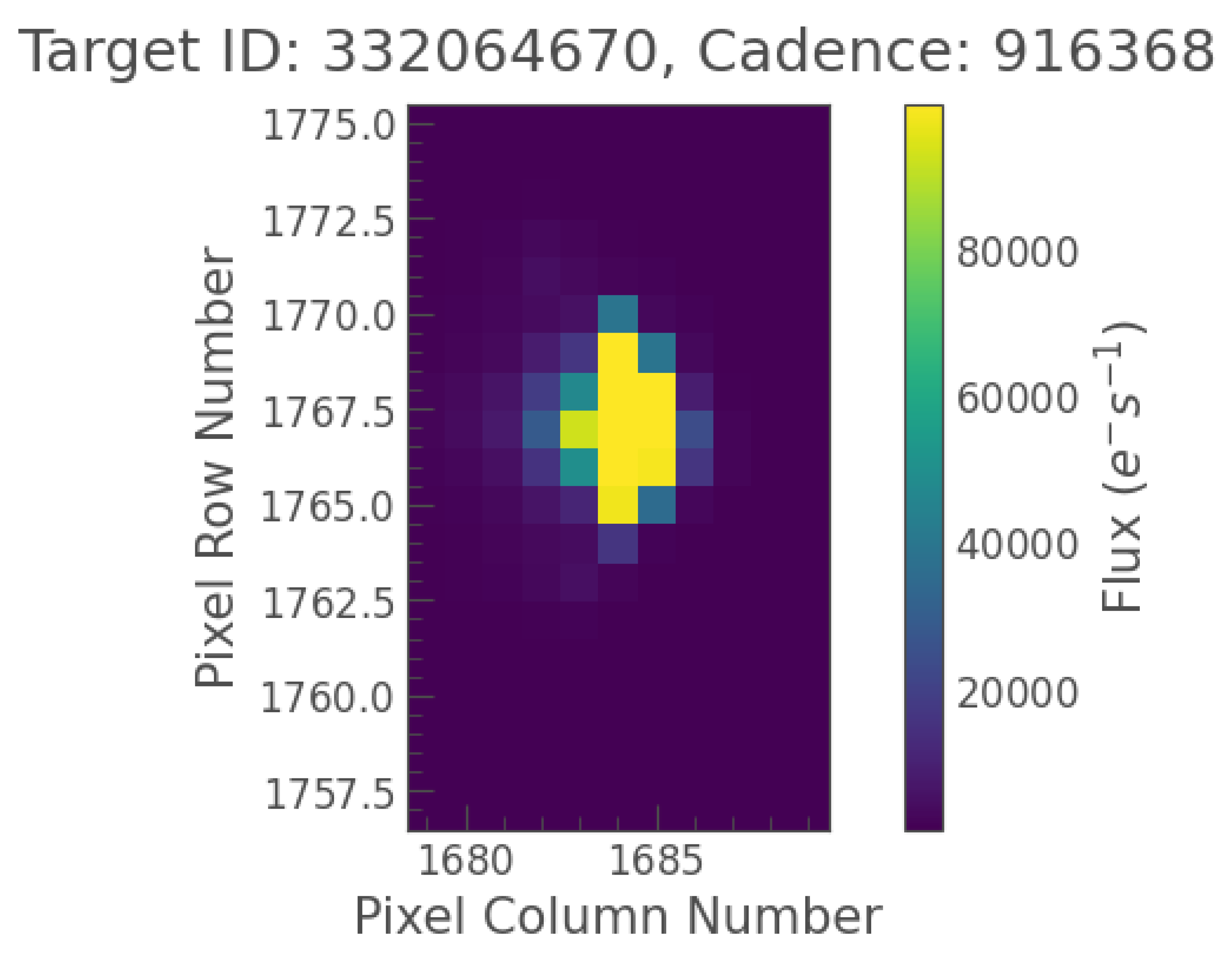
We retrieved the data for each observation period from the MAST archive, and first examined the raw target pixel file to ensure the data was accessible for processing. An example of the pixel data from this system can be seen in Figure 1.

2.3. Data Processing and Analysis

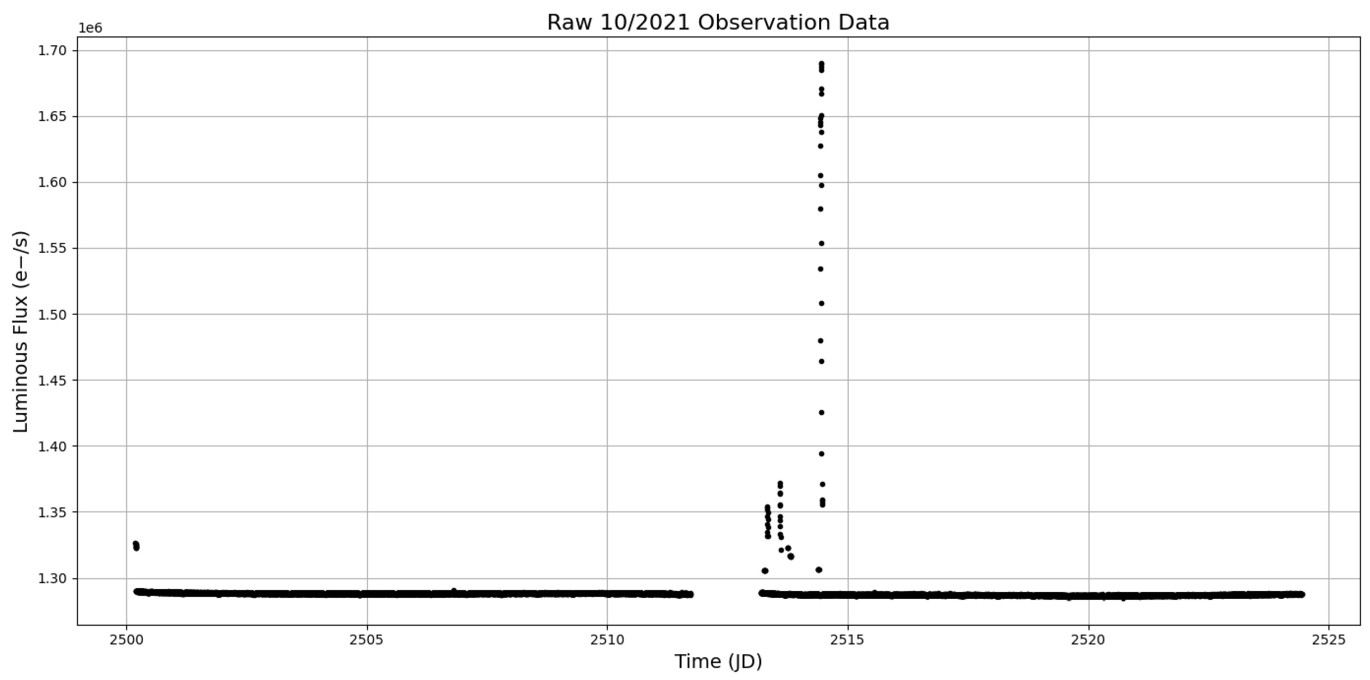
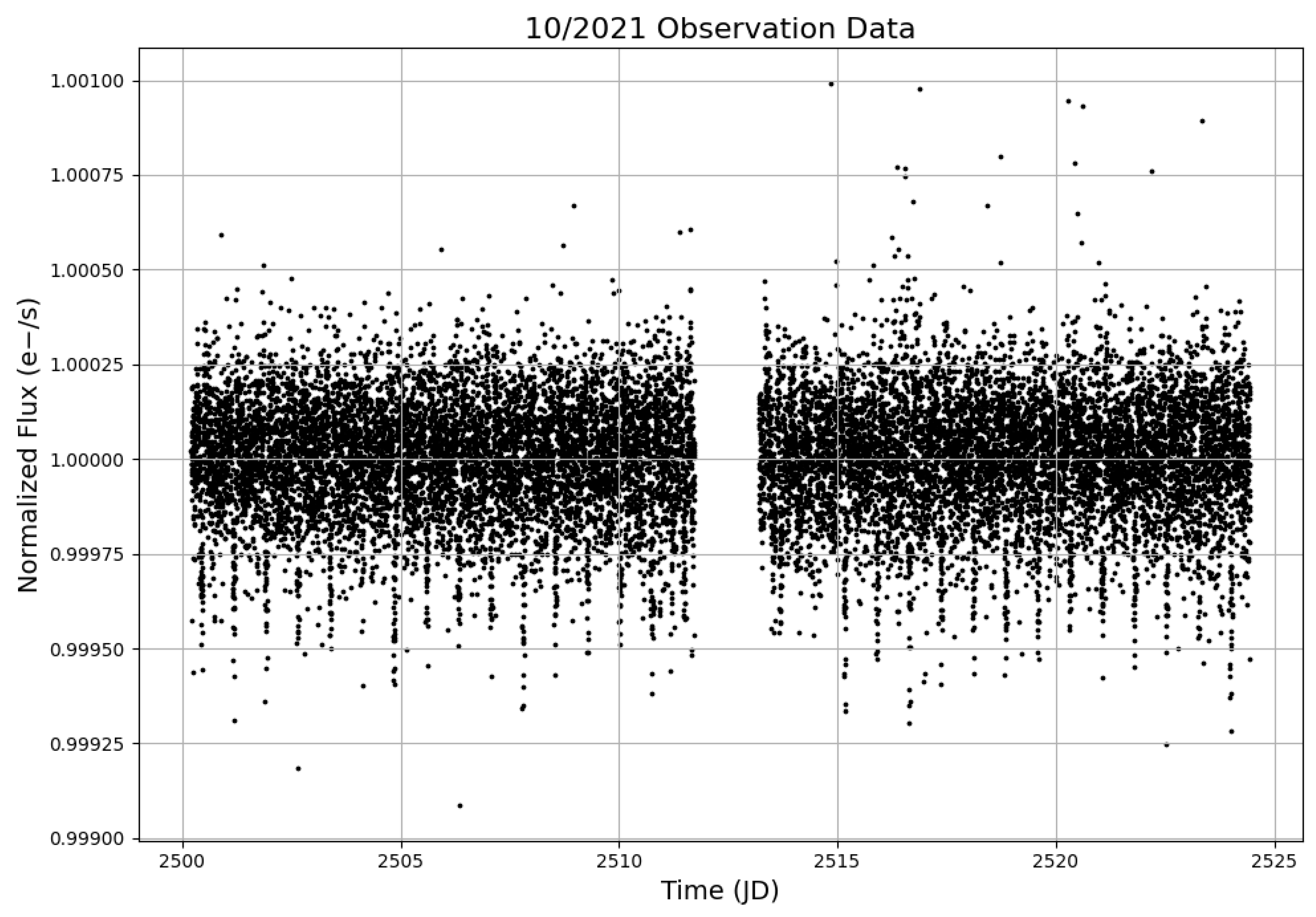
When initially extracted from the archive, the raw data contains periods of sharp variations in flux which are much larger than the luminosity dips due to planetary transits (see Figure 2). Using a Python 3.11.15 package named Lightkurve [24], we applied a Savitzky-Golay filter with a two degree polynomial to remove outliers from the data which were more than 4 standard deviations from the average flux. This filter also removed long-range variation in the flux not due to transit effects and normalized the flux to a constant value (set as 1) with dips in the flux due to transits expressed as a fraction of this normalized value (see Figure 3). The data inside each transit was not masked before detrending, instead the window size for the filter was set to be large enough (401) in order not to affect the measured transit depth.

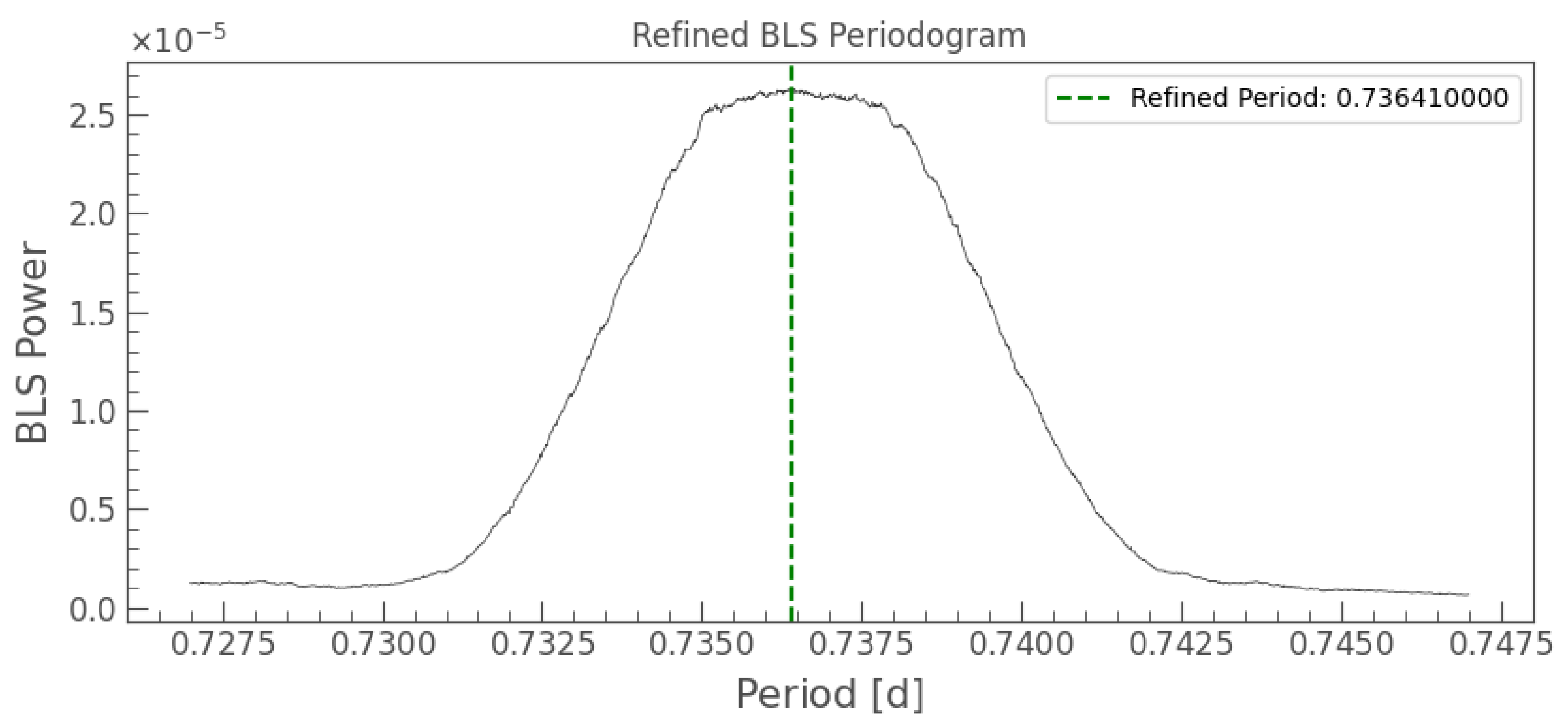
We then applied a box least-squared periodogram, first with a larger range and step size, and then using a finer range and step size centered on the result of the first stage, which returned a value for the orbital period of the planet of 0.7364 days (see Figure 4). This is consistent with the value of 0.7365 days found by Dawson and Fabrycky [12].

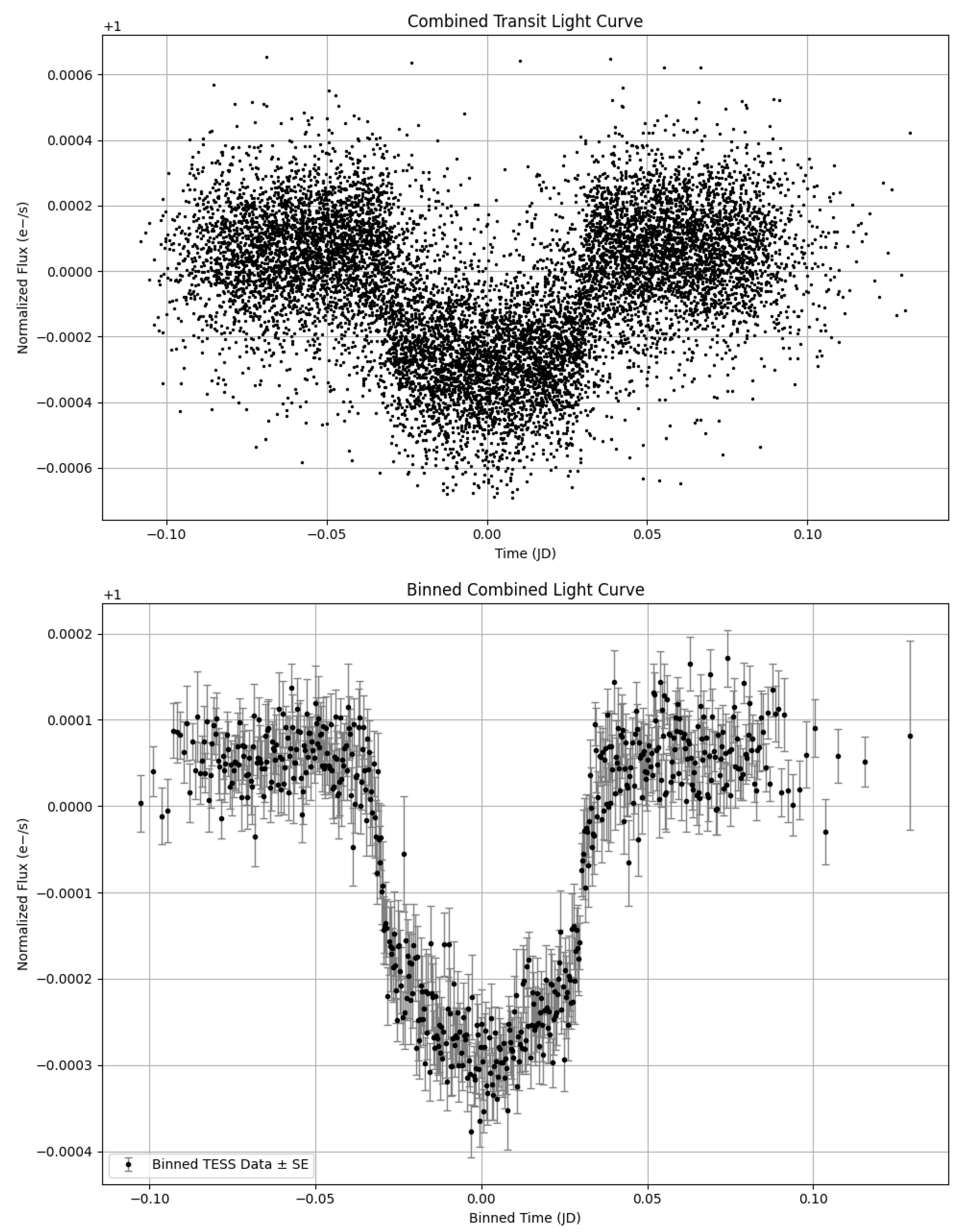
We isolated the transits from each of the three TESS observations into 5 h segments centered around the midpoint of each of the transits. We then overlaid all of the individual transits with each transit midpoint being set at time $t=0$. The data from all of the overlaid transits were added together into a single dataset for fitting and analysis. Next, we binned the combined plot in time with a bin size of 20 data points per bin. This corresponded to an average time duration of 24 s for each binned data point. The curvature due to limb darkening is somewhat visible in the unbinned plot, and becomes significantly more obvious after the binning has been applied (see Figure 5, top/bottom).

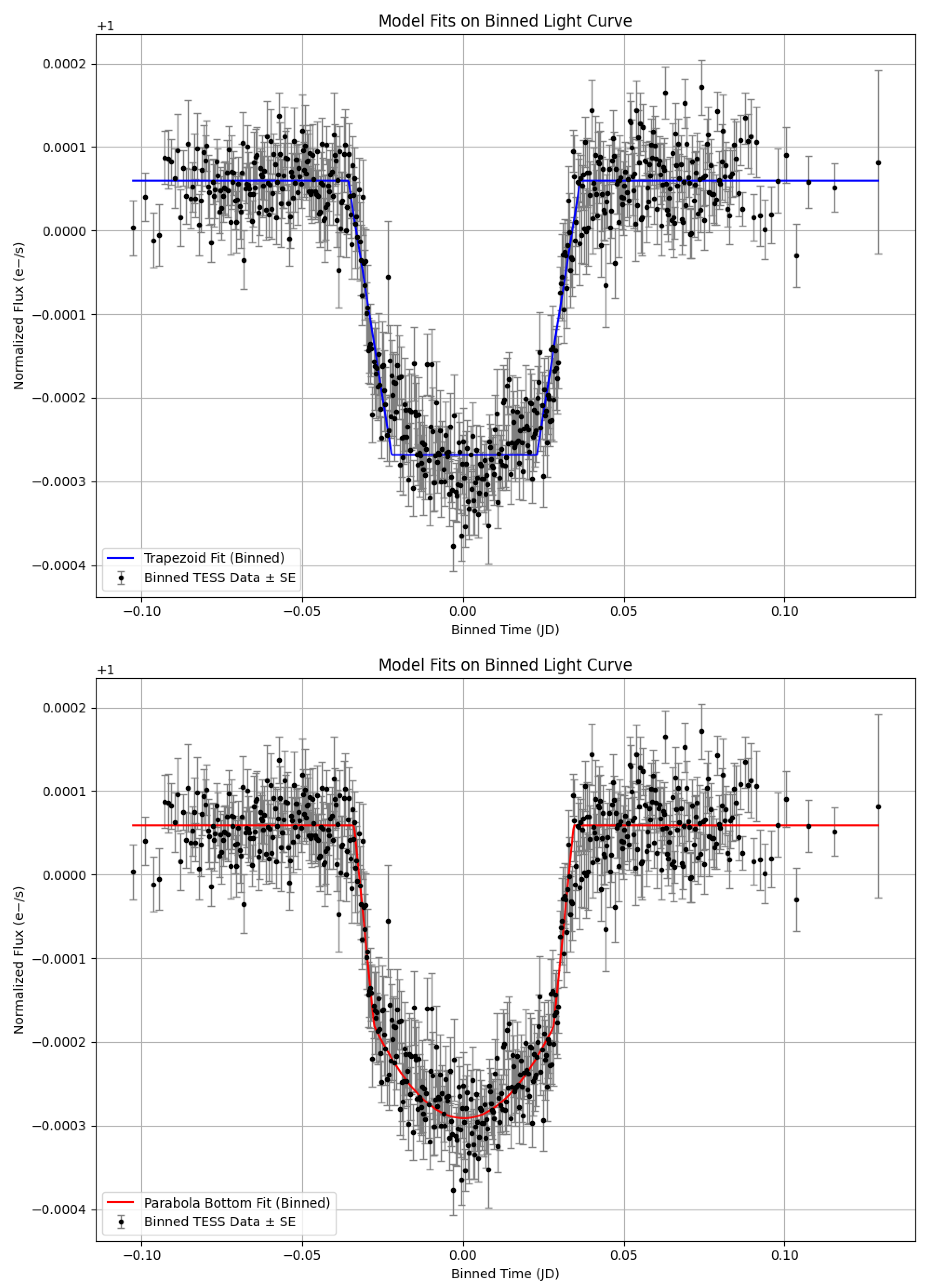
We then applied two different piecewise polynomial fits to the data in order to determine the statistical significance of the curvature. The curvature of the combined transit data is most visible in the binned dataset, as evident by the reduced ${\chi }^2$ values for the fits. The flat-bottomed (trapezoidal) fit with no allowance for curvature due to limb darkening (Figure 6 (top)) has a reduced ${\chi }^2$ value of 1.357 while the parabolically-bottomed fit which allows for curvature due to limb darkening (Figure 6 (bottom)) has a significantly smaller reduced ${\chi }^2$ value of 1.152. The parabolically-bottomed fit is thus significantly more likely to describe the data than the flat-bottomed (trapezoidal) fit. In fact, we found that the parabolically-bottomed fit had a reduced ${\chi }^2$ value not only in comparison to the flat-bottomed fit, but also in comparison to the BATMAN fit described later. This is primarily due to the use of only one single curvature parameter in the parabolic approximation, as opposed to the large number of parameters in the BATMAN fit.

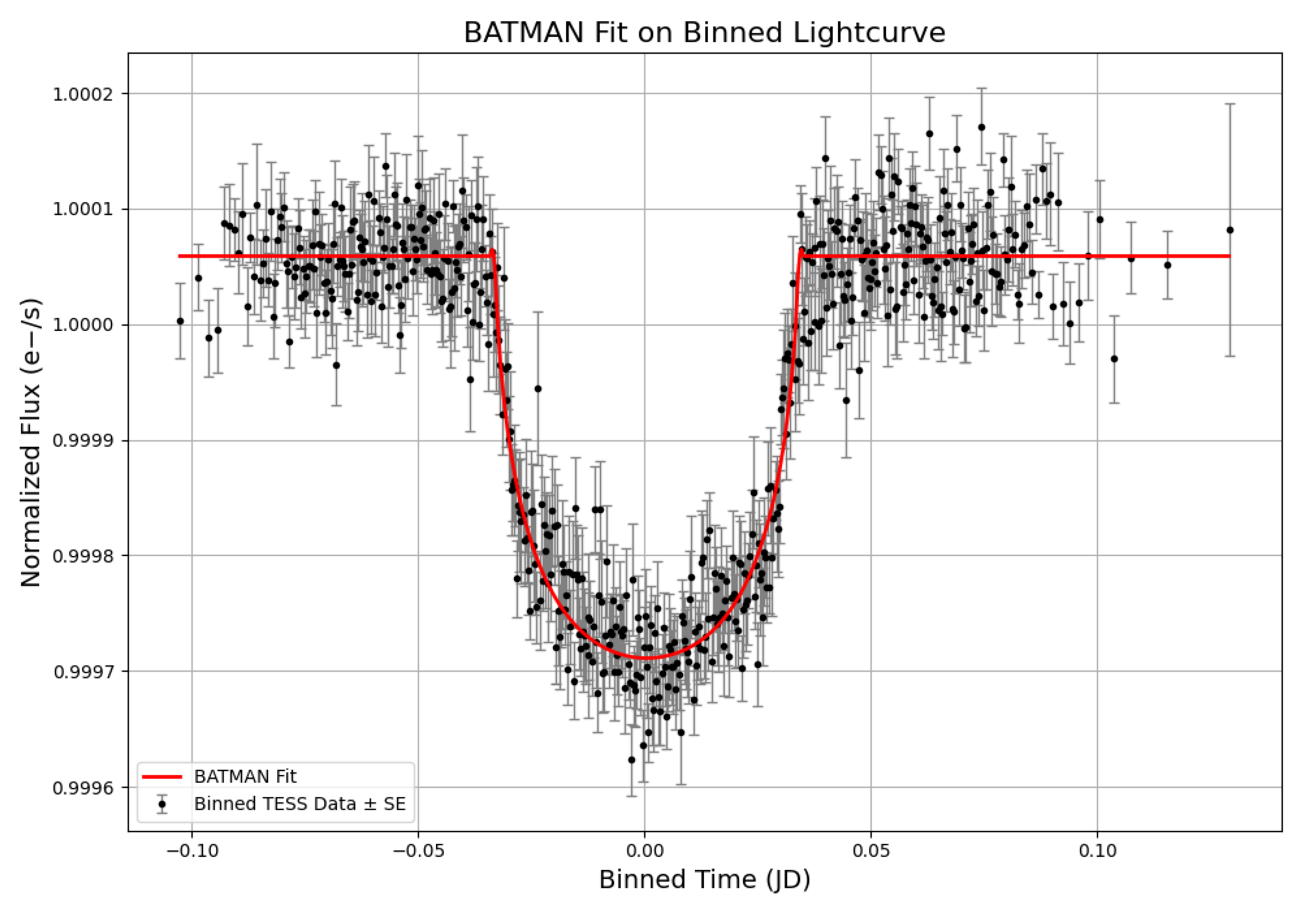
To quantify the statistical significance of our observation of the curvature due to limb darkening, we applied a maximum likelihood test to the piecewise polynomial fits done using Python. Using the logarithmic likelihood, the difference in the Bayesian Information Criterion ($\mathrm{\Delta }$BIC) between the two fits is 106.67, showing that the parabolically bottomed fit is approximately 1000 times more likely to represent the data than the flat-bottomed fit. To reparameterize our curvature to the form of Equation (1), we used a Python package called BATMAN (BAsic Transit Model cAlculatioN in Python), specifically designed for fitting transit light curves. A detailed description of BATMAN can be found in the reference by Kreidberg [25] which is based on a theoretical limb darkening model by Mandel [9]. The BATMAN fit (see Figure 7) resulted in a reduced ${\chi }^2$ value of 1.20 and a ($\mathrm{\Delta }$BIC) of 74.92 in favor of the BATMAN fit as compared to the flat-bottomed fit.

3. Results

By using the trapezoidal (flat-bottomed) and parabolically bottomed fits, we were able to estimate the parameters related to the time, depth, and duration of the transit, as well as the duration of the ingress/egress portions of the transit, and the baseline level of the flux outside of the transit in terms of the overall normalized flux. For the trapezoidal (flat-bottomed) fit, the curvature of the light curve during the transit (i.e., between ingress and egress) was set to be zero by definition, but for the parabolically bottomed fit, the curvature parameter at the transit bottom was determined by the fit. The full results of the transit parameters found by the trapezoidal and parabolic fits can be found in

Table 2. Trapezoidal and parabolic parameter results from fits.

Parameter	Trapezoid Fit	Parabolic Bottom Fit
$t_0$ (days)	$0.000414\pm 0.000158$	$0.000306\pm 0.000149$
Normalized Depth	$0.000328\pm 0.00003$	$0.000240\pm 0.000009$
Duration (days)	$0.072116\pm 0.000625$	$0.068308\pm 0.000622$
Ingress (days)	$0.013463\pm 0.000542$	$0.006204\pm 0.000621$
Normalized Baseline	$1.000060\pm 0.000002$	$1.000059\pm 0.000002$

Normalized curvature at transit bottom: $0.282793\pm 0.030816$.

and the goodness-of-fit results for the trapezoidal and parabolic fits can be found in

Table 3. Trapezoidal and parabolic goodness of fit results.

Fit Type	${\chi }^2$		Reduced ${\chi }^2$
Trapezoid Fit	741.1266576		1.3573748292
Parabola Bottom Fit	628.1461862		1.1525618690
Fit Type	$logL$	AIC	BIC
Trapezoid Fit	4779.3811	−9548.76	−9527.20
Parabolic Fit	4835.8714	−9659.74	−9633.87

BIC Difference: $106.67$ (favoring parabolic model over trapezoidal).

.

Here, $t_0$ is the time of the center of the transit from the fit of the combined data set relative to the time of the center of each individual transit. The small values indicate a high degree of consistancy in the identification of the transit center.

In Table 3, $logL$ is the log likelihood value, and $AIC$ is the Akaike Information Criterion, which penalizes the likelihood value by $2k-2ln\left(L\right)$, where k is the number of parameters and L is the log likelihood. $BIC$ is the Bayesian information criterion, which penalizes the likelihood value by $k\ast ln\left(n\right)-2ln\left(L\right)$, where k and L are defined as in the $AIC$ and n is the number of data points. $BIC$ is stricter and results in lower values for more parameters compared to $AIC$, and as such the difference between two goodness-of-fit results is reported in terms of $\mathrm{\Delta }BIC$.

Using BATMAN to fit the binned data set, we were able to find values for the orbital parameters of 55 Cancri e. In

Table 4. BATMAN Transit Model Orbital Parameters.

Parameter	Value	Uncertainty (1$\mathit{\sigma }$)
Inclination (degrees)	$84.930185$	$16.546900$
Impact parameter ($b=acosi$)	$0.388326$	$1.277558$

, a is the semi-major axis of the planet’s orbit in units of stellar radii, $r_p$ is the planetary radius in units of stellar radii, and the normalized baseline is fit parameter for the average value of the flux outside of the transit periods. This was made a fitted parameter in our analysis to enable the fits to converge. The inclination of the orbit is given in degrees, where 90 degrees represents a transit across the equator. From the BATMAN fit we obtained a value of the inclination of the orbit of $85\pm 17$ degrees and a value for the impact parameter of $0.4\pm 1.3$ (see Table 4). The relatively large uncertainty in the BATMAN fit for the orbital inclination was correlated with relatively large uncertainties for other parameters, in particular the limb darkening coefficients. For the planetary radius, the BATMAN fit resulted in a value of $r_p=0.016\pm 0.003$ where $r_p$ is the ratio of the planetary radius to the stellar radius, and for the semi-major axis of the orbit expressed in terms of the stellar radius the BATMAN fit resulted in a value of $a/r_{stellar}=4.4\pm 2.1$. Using the stellar radius result for 55 Cnc from von Braun et al. [22] we obtain a planetary radius of $1.64\pm 0.10$ earth radii, and an orbital radius of $0.019\pm 0.009$ AU. This planetary radius is somewhat smaller than the the value of $1.88\pm 0.03$ observed by Bourrier et al. in 2018 [13]. We were also able to use the BATMAN fit to the binned light curve to obtain the quadratic limb darkening coefficients $u_1$ and $u_2$, albeit with large uncertainties. Using the original BATMAN fit results we obtained a value for $u_1$ of $0.56\pm 0.57$ and for $u_2$ we obtained a value of $0.62\pm 0.69$ (see

Table 5. BATMAN Transit Model Fit Results—The ${\chi }^2$ for the fit is 653.582 and the reduced ${\chi }^2$ is 1.201.

Parameter	Value	Uncertainty (1$\mathit{\sigma }$)
$t_0$ (days)	0.000508	0.000150
$r_p/r_{stellar}$	0.016107	0.003161
$a/r_{stellar}$	4.394337	2.092066
$u_1$	0.556642	0.568146
$u_2$	0.624010	0.685011
Normalised baseline	1.000059	0.000002

). Adjusting the bounds on the fit gave a result with slightly lower uncertainties, with $u_1=0.54\pm 0.48$ and $u_2=0.64\pm 0.55$. These values, rather than the results from the original fit attempt in Table 5, are the results reported in our abstract. Additional strategies to reduce the uncertainties are discussed in the following section.

4. Discussion

The statistical results from our trapezoidal and parabolically bottomed fits showed that the shape of the light curve during transit must be due to the effects of limb darkening and can not simply be a result of random variation in the flux. This allowed us to attempt to fit for the full range of transit parameters, including planetary radius, orbital size, orbital inclination, impact parameter, as well as the limb darkening coefficients $u_1$ and $u_2$.

From the results of the fit using BATMAN we obtained values for the physical and orbital parameters of 55 Cancri e. These values were by and large similar to those previously reported, although with some differences in the uncertainties. One significantly different parameter was the planetary radius of 55 Cancri e for which we report a result of $1.64\pm 0.1$ earth radii, which is slightly smaller than the result of $1.88\pm 0.03$ reported by Bourrier et al. in 2018 [13]. Our results for orbital inclination, $(85\pm 17)$ degrees, were somewhat better constrained than that of Bourrier et al., which reported $\left({85}_{-33}^{+31}\right)$ degrees. The results of our fits as compared to those of Bourrier et al. are summarized in

Table 6. Comparison of results with those of Bourrier et al. [13].

Parameter	This Work	Bourrier et al.
Inclination (degrees)	$(85\pm 17)$	$\left({85}_{-33}^{+31}\right)$
$r/r_{earth}$	$1.64\pm 0.10$	$1.88\pm 0.03$
a (AU)	$0.019\pm 0.009$	$0.0154\pm 0.0001$
$u_1$	$0.58\pm 0.48$	$0.544\pm 0.008$
$u_2$	$0.64\pm 0.55$	$0.186\pm 0.004$

.

Our fit was less successful than Bourrier et al. in obtaining values for $u_1$ and $u_2$, the limb darkening coefficients of 55 Cancri A, however it should be noted that Bourrier et al. did not directly fit $u_1$ and $u_2$ but instead replaced the inclination by its cosine, and the limb-darkening coefficients by the linear combinations $c_1=2u_1+u_2$ and $c_1=u_1-2u_2$ [13].

We used ExoCTK as the limb darkening coefficient calculator, and compared our results to the Kurucz ATLAS9 model across the TESS waveband [6,7,8]. The expected values of the coefficients from the Kurucz ATLAS9 model did fall within the range of our measurements [13,26], but the uncertainties in our values were much greater than those reported by Bourrier et al. for 55 Cancri in 2018 using HST/STIS observations [13], which reported values of $u_1=0.544\pm 0.008$ and $u_2=0.186\pm 0.004$. We note that in terms of the reduced ${\chi }^2$, the effective parametrization $I^{\prime }\left(t\right)=C\left(t^2\right)$ returned a lower value (1.153 vs. 1.201), as well as a $\mathrm{\Delta }BIC$ difference of 31.75 in favor of the effective parametrization. We report the results of our effective parametrization of the curvature of the transit lightcurve primarily because this parametrization is favored by our goodness-of-fit tests, and not because it is motivated by any particular stellar model. We also note that the single curvature parameter from our effective parametrization, $C\left(t^2\right)=0.28\pm 0.03$, has a significantly lower relative uncertainty than those of our values for the quadratic limb darkening coefficients, for which we obtained $u_1=0.58\pm 0.48$ and $u_2=0.64\pm 0.55$. The goodness-of-fit results are summarized in

Table 7. Goodness-of-Fit Results for the flat-bottomed, parabolically bottomed, and BATMAN models.

Fit Type	Reduced ${\mathit{\chi }}^2$	$\mathit{BIC}$
Flat-bottomed	1.357	−9633.87
BATMAN	1.201	−9559.62
Parabolically-bottomed	1.152	−9527.87

.

The next step in our research into the 55 Cancri system is to reduce the size of the uncertainties in our values, particularly for the limb darkening coefficients. One approach would be to reduce the number of free parameters in the BATMAN fit by using values for parameters such as orbital inclination taken from other sources. A Markov Chain Monte Carlo optimization may also be better able to handle the correlation between parameters as compared to the polynomial optimization used in this research. The errors could also be improved by including additional data from later TESS observational runs into the fit, as the relatively smaller amount of data currently available in the regions of ingress and egress, particularly at the point at which the planet begins to enter the disk of the star, may have an outsized impact on the accuracy of the results. Incorporating additional observational periods may be helpful to reduce the uncertainties in some of the parameters.

References

1. Vanderspek, R.; Doty, J.; Fausnaugh, M.; Villasenor, J.N.S.; Jenkins, J.M.; Berta-Thompson, Z.K.; Burke, C.J.; Ricker, G.R. TESS Instrument Handbook v0.1. 2018. Available online: https://archive.stsci.edu/files/live/sites/mast/files/home/missions-and-data/active-missions/tess/_documents/TESS_Instrument_Handbook_v0.1.pdf (accessed on 20 December 2025).
2. Sullivan, P.W.; Winn, J.N.; Berta-Thompson, Z.K.; Charbonneau, D.; Deming, D.; Dressing, C.D.; Latham, D.W.; Levine, A.M.; McCullough, P.R.; Morton, T.; et al. The transiting exoplanet survey satellite: Simulations of planet detections and astrophysical false positives. Astrophys. J. 2015, 809, 77. [Google Scholar] [CrossRef]
3. Ricker, G.R.; Winn, J.N.; Vanderspek, R.; Latham, D.W.; Bakos, G.Á.; Bean, J.L.; Berta-Thompson, Z.K.; Brown, T.M.; Buchhave, L.; Butler, N.R.; et al. Transiting Exoplanet Survey Satellite (TESS). J. Astron. Telesc. Instrum. Syst. 2015, 1, 014003. [Google Scholar] [CrossRef]
4. Deeg, H.J.; Alonso, R. Transit Photometry as an Exoplanet Discovery Method. arXiv 2018, arXiv:1803.07867. [Google Scholar]
5. Winn, J.N. Exoplanet Transits and Occultations. arXiv 2010, arXiv:1001.2010. [Google Scholar]
6. Claret, A.; Bloemen, S. Limb Darkening Coefficients for the Kepler, CoRoT, Spitzer, UV, Optical, and IR Passbands. Astron. Astrophys. 2011, 529, A75. [Google Scholar] [CrossRef]
7. STScI. ExoCTK Limb Darkening Calculator. 2025. Available online: https://exoctk.stsci.edu/limb_darkening (accessed on 20 December 2025).
8. Wade, R.A.; Rucinski, S.M. Linear and quadratic limb-darkening coefficients for a large grid of LTE model atmospheres. Astron. Astrophys. Suppl. Ser. 1985, 60, 471–484. [Google Scholar]
9. Mandel, K.; Agol, E. Analytic Light Curves for Planetary Transit Searches. Astrophys. J. Lett. 2002, 580, L171. [Google Scholar] [CrossRef]
10. McArthur, B.E.; Endl, M.; Cochran, W.D.; Benedict, G.F.; Fischer, D.A.; Marcy, G.W.; Butler, R.P.; Naef, D.; Mayor, M.; Queloz, D.; et al. Detection of a Neptune-Mass Planet in the ρ1 Cancri System Using the Hobby-Eberly Telescope. Astrophys. J. Lett. 2004, 614, L81. [Google Scholar] [CrossRef]
11. Fischer, D.A.; Marcy, G.W.; Butler, R.P.; Vogt, S.S.; Laughlin, G.; Henry, G.W.; Abouav, D.; Peek, K.M.G.; Wright, J.T.; Johnson, J.A.; et al. Five Planets Orbiting 55 Cancri. Astrophys. J. 2008, 675, 790. [Google Scholar] [CrossRef]
12. Dawson, R.I.; Fabrycky, D.C. Radial Velocity Planets De-aliased: A New, Short Period for Super-Earth 55 Cnc e. Astrophys. J. 2010, 722, 937. [Google Scholar] [CrossRef]
13. Bourrier, V.; Dumusque, X.; Dorn, C.; Henry, G.W.; Astudillo-Defru, N.; Rey, J.; Benneke, B.; Hébrard, G.; Lovis, C.; Demory, B.O.; et al. The 55 Cancri system reassessed. Astron. Astrophys. 2018, 619, A1. [Google Scholar] [CrossRef]
14. Meier Valdés, E.A.; Morris, B.M.; Wells, R.D.; Schanche, N.; Demory, B.-O. Weak evidence for variable occultation depth of 55 Cnc e with TESS. Astron. Astrophys. 2022, 663, A95. [Google Scholar] [CrossRef]
15. Demory, B.O.; Gillon, M.; Deming, D.; Valencia, D.; Seager, S.; Benneke, B.; Lovis, C.; Cubillos, P.; Harrington, J.; Stevenson, K.; et al. Detection of a transit of the super-Earth 55 Cancri e with warm Spitzer. Astron. Astrophys. 2011, 533, A114. [Google Scholar] [CrossRef]
16. Demory, B.O.; Seager, S.; Madhusudhan, N.; Kjeldsen, H.; Christensen-Dalsgaard, J.; Gillon, M.; Rowe, J.F.; Welsh, W.F.; Adams, E.R.; Dupree, A.; et al. The high albedo of the hot Jupiter Kepler-7 b. Astrophys. J. Lett. 2011, 735, L12. [Google Scholar] [CrossRef]
17. Demory, B.O.; Gillon, M.; De Wit, J.; Madhusudhan, N.; Bolmont, E.; Heng, K.; Kataria, T.; Lewis, N.; Hu, R.; Krick, J.; et al. A map of the large day–night temperature gradient of a super-Earth exoplanet. Nature 2016, 532, 207–209. [Google Scholar] [CrossRef]
18. Demory, B.O.; Gillon, M.; Madhusudhan, N.; Queloz, D. Variability in the super-Earth 55 Cnc e. Mon. Not. R. Astron. Soc. 2016, 455, 2018–2027. [Google Scholar] [CrossRef]
19. Tamburo, P.; Mandell, A.; Deming, D.; Garhart, E. Confirming variability in the secondary eclipse depth of the super-Earth 55 Cancri e. Astron. J. 2018, 155, 221. [Google Scholar] [CrossRef]
20. Winn, J.N.; Matthews, J.M.; Dawson, R.I.; Fabrycky, D.; Holman, M.J.; Kallinger, T.; Kuschnig, R.; Sasselov, D.; Dragomir, D.; Guenther, D.B.; et al. A Super-Earth Transiting a Naked-Eye Star. Astrophys. J. Lett. 2011, 737, L18. [Google Scholar] [CrossRef]
21. Ehrenreich, D.; Bourrier, V.; Bonfils, X.; Des Etangs, A.L.; Hébrard, G.; Sing, D.K.; Wheatley, P.J.; Vidal-Madjar, A.; Delfosse, X.; Udry, S.; et al. Hint of a transiting extended atmosphere on 55 Cancri b. Astron. Astrophys. 2012, 547, A18. [Google Scholar] [CrossRef]
22. von Braun, K.; Boyajian, T.S.; ten Brummelaar, T.A.; Kane, S.R.; van Belle, G.T.; Ciardi, D.R.; Raymond, S.N.; López-Morales, M.; McAlister, H.A.; Schaefer, G.; et al. 55 Cancri: Stellar Astrophysical Parameters, a Planet in the Habitable Zone, and Implications for the Radius of a Transiting Super-Earth. Astrophys. J. 2011, 740, 49. [Google Scholar] [CrossRef]
23. Yee, S.W.; Petigura, E.A.; von Braun, K. Precision Stellar Characterization of FGKM Stars using an Empirical Spectral Library. Astrophys. J. 2017, 836, 77. [Google Scholar] [CrossRef]
24. Collaboration, L.; Cardoso, J.V.d.M.; Hedges, C.; Gully-Santiago, M.; Saunders, N.; Cody, A.M.; Barclay, T.; Hall, O.; Sagear, S.; Turtelboom, E.; et al. Lightkurve: Kepler and TESS time series analysis in Python. Astrophysics Source Code Library. arXiv 2018, arXiv:1812.013. Available online: http://ui.adsabs.harvard.edu/abs/2018ascl.soft12013L (accessed on 20 December 2025).
25. Kreidberg, L. batman: BAsic Transit Model cAlculatioN in Python. Publ. Astron. Soc. Pac. 2015, 737, L18. [Google Scholar] [CrossRef]
26. Patel, J.A.; Espinoza, N. Empirical limb-darkening coefficients & transit parameters of known exoplanets from TESS. Astron. J. 2022, 163, 301. [Google Scholar] [CrossRef]
Figure 1. Target pixel file from the 10/2021 TESS observation period.
Astronomy 05 00003 g001
Figure 2. Raw lightcurve from the 10/2021 TESS observation period. Note the large spikes in flux which must be removed to observe the smaller variations due to transits. The thick horizontal black line represents the data which remains after the large spikes in the flux are removed.
Astronomy 05 00003 g002
Figure 3. Lightcurve from the 10/2021 TESS observation after applying the Savitsky-Golay filter and normalization. The large number of individual transits are now visible as individual dips from the thick black band of luminosities observed outside of transit.
Astronomy 05 00003 g003
Figure 4. Refined periodogram for the 10/2021 dataset.
Astronomy 05 00003 g004
Figure 5. (Top) Unbinned combined transit light curve plot. (Bottom) Combined light curve with a bin size of 20 points per bin. Black circles represent the mean value for each bin. Error bars are statistical and calculated from the bin.
Astronomy 05 00003 g005
Figure 6. (Top) Flat-bottomed (trapezoidal) polynomial fit on the binned data set. (Bottom) Parabolically-bottomed polynomial fit on the binned data set.
Astronomy 05 00003 g006
Figure 7. BATMAN fit on the binned combined light curve.
Astronomy 05 00003 g007