On the Possible Nature of White Holes

Abstract

This paper considers non-singular black holes. It discusses the observation of particles falling onto ordinary and non-singular black holes from the perspective of a distant observer. It is demonstrated that, during a stage in the evolution of non-singular black holes, powerful energy fluxes can be emitted. Distant observers may interpret these fluxes as white holes.

1. Introduction

About 50 years ago, on the basis of an analysis of Einstein’s equations, Novikov showed that in the universe, along with black holes, radiation from which is impossible, there must be white holes, which cannot be reached from outside [1,2,3]. Moreover, pure black holes or pure white holes cannot exist. In other words, all matter drawn into a black hole splashes out either into the neighboring universe, for which it is white, or a so-called wormhole is formed—a bridge along which matter drawn into a black hole from one area of the universe splashes out through a white hole into another. In the astrophysical community, quasars [3] and powerful short-lived bursts of gamma radiation [4,5] are considered as candidates for a white hole. The question of the existence (or rather the possibility of detection) of white holes is open, since at the edge of the event horizon of a white hole, the density of matter should reach such a high value that black holes should form, which “eat” the matter flowing out of the white [6].

In [7], we proposed a cavitation model of the inflationary stage of the Big Bang. In this model, following the work of Guth [8], the effect of the cosmological Λ-term is considered as a source of negative pressure acting in the region of a false vacuum, in which, because of the tunneling phase transition, bubbles of the physical vacuum appear, in which the cosmological constant is equal to zero. This process is similar to the tunneling regime of transition to cavitation in cryogenic liquid helium in the region of negative pressure [9]. The cavitation model of the inflationary stage [7] makes it possible to explain the homogeneity and large-scale isotropy of the universe without generating unrelated space-time universes and to explain the large-scale cellular structure of the universe.

In [10,11,12] were shown that within the framework of the general theory of relativity, there are no solutions in which there is no matter on the border of the false and physical vacuums. In other words, when bubbles of physical vacuum (empty space) are formed in a false vacuum, there is always a narrow region of gravitating matter at their interface. As shown in [7], under certain conditions the formation of event horizons arises at this boundary [3]. As shown in [7], bubbles of the physical vacuum displace the false one in a finite time, so that the exponential (inflationary) expansion of the universe smoothly turns into the usual expansion predicted by Gamov [13]. It is possible that with the formation of bubbles of a physical vacuum in a false one, structures can be formed in which the false vacuum is inside a shell of gravitating matter. In this case, singular-free black holes described in [8] can arise. The difference between singular-free black holes with a false vacuum region inside and singular-free holes considered in [14,15] is that the absence of a singularity in the latter is associated with a specific density distribution of gravitating matter.

The Structure of This Paper Is as Follows:

Part 2 contains the equations for nonsingular black holes. Part 3 considers the passage of particles through the horizon from the perspective of a distant observer. We show that, in this frame of reference, the wave properties of particles approaching the horizon begin to play a dominant role. This allows us to estimate the time it takes particles to pass through the event horizon as observed in a distant reference frame. Part 4 generalizes the results of Part 3 to particle motion in the field of a singular black hole. Part 5 considers the accretion onto nonsingular black holes and the resulting radiation.

2. Mathematical Model of Non-Singular Black Holes

Consider the space-time metric in the frame of reference associated with the center of a spherical false vacuum surrounded by a true vacuum. Following [16,17], we will consider the transition region at the border of the false and physical vacuums in the De Sitter metric. According to [18], the expression for the interval ds in the centrally symmetric case, in terms of the variables $t$, $r$, and $\theta$, $\varphi$, is given by:

$$d{s}^2=e^v{c}^{2}d{t}^2-e^{\lambda }d{r}^2-r^2\left(d{\theta }^2+{sin}^2\theta d{\varphi }^2\right).$$

(1)

In this case, Einstein’s equations, taking into account the cosmological term, are converted to form [7,18]:

$${\displaystyle \frac{8\pi G}{c^4}}{T}_0^0-\Lambda =-e^{-\lambda }\left({\displaystyle \frac{1}{r^2}}-{\displaystyle \frac{{\lambda }^{\prime }}{r}}\right)+{\displaystyle \frac{1}{r^2}}.$$

(2)

$${\displaystyle \frac{8\pi G}{c^4}}{T}_1^1-\Lambda =-e^{-\lambda }\left({\displaystyle \frac{{\nu }^{\prime }}{r}}+{\displaystyle \frac{1}{r^2}}\right)+{\displaystyle \frac{1}{r^2}}$$

(3)

$${\displaystyle \frac{8\pi G}{c^4}}{T}_2^2-\Lambda ={\displaystyle \frac{8\pi G}{c^4}}{T}_3^3-{\displaystyle \frac{1}{c^2}}\Lambda =-{\displaystyle \frac{1}{2}}{e}^{-\lambda }\left({\nu }^{″}+{\displaystyle \frac{{\nu }^{\prime 2}}{2}}+{\displaystyle \frac{{\nu }^{\prime }-{\lambda }^{\prime }}{r}}-{\displaystyle \frac{{\nu }^{\prime }{\lambda }^{\prime }}{2}}\right)+{\displaystyle \frac{1}{2}}{e}^{-\nu }\left(\ddot{\lambda }+{\displaystyle \frac{{\dot{\lambda }}^2}{2}}-{\displaystyle \frac{\dot{\lambda }\dot{\nu }}{2}}\right)$$

(4)

$${\displaystyle \frac{8\pi G}{c^4}}{T}_0^1={\displaystyle \frac{8\pi G}{c^4}}{T}_1^0=-e^{-\lambda }{\displaystyle \frac{\dot{\lambda }}{r}}$$

(5)

In (2)–(5) $T_k^i$ is the energy-momentum tensor, $\Lambda$ is the cosmological term introduced by Einstein in the equations of the General Theory of Relativity, $c$ is speed of light, $G$ is the gravitational constant. The dots above $\lambda$ and $\nu$ are the derivatives with respect to time, and the primes—the derivative with respect to the coordinate $r$.

In the stationary case, when the coefficients $v$, $\lambda$ do not depend on $t$, Einstein’s equations take the following form:

$${\displaystyle \frac{8\pi G}{{\mathrm{c}}^4}}{T}_0^0={\displaystyle \frac{8\pi G}{c^4}}{\tilde{T}}_0^0-\Lambda =-e^{-\lambda }\left({\displaystyle \frac{1}{r^2}}-{\displaystyle \frac{{\lambda }^{\prime }}{r}}\right)+{\displaystyle \frac{1}{r^2}}.$$

(6)

$${\displaystyle \frac{8\pi G}{c^4}}{T}_1^1={\displaystyle \frac{8\pi G}{c^4}}{\tilde{T}}_1^1-\Lambda =-e^{-\lambda }\left({\displaystyle \frac{{\nu }^{\prime }}{r}}+{\displaystyle \frac{1}{r^2}}\right)+{\displaystyle \frac{1}{r^2}}$$

(7)

$${\displaystyle \frac{8\pi G}{c^4}}{T}_2^2={\displaystyle \frac{8\pi G}{c^4}}{\tilde{T}}_2^2-\Lambda ={\displaystyle \frac{8\pi G}{c^4}}{\tilde{T}}_3^3-\Lambda =-{\displaystyle \frac{1}{2}}{e}^{-\lambda }\left({\nu }^{\prime \prime }+{\displaystyle \frac{{\nu }^{\prime 2}}{2}}+{\displaystyle \frac{{\nu }^{\prime }-{\lambda }^{\prime }}{r}}-{\displaystyle \frac{{\nu }^{\prime }{\lambda }^{\prime }}{2}}\right).$$

(8)

All other components of $T_k^i$ are equal to zero.

Putting as in [7,15] $\nu =-\lambda$, we obtain the system of equations:

$${\displaystyle \frac{d}{dr}}\left({re}^{-\lambda }\right)=1-r^2\left({\displaystyle \frac{8\pi G}{c^4}}{T}_0^0-\Lambda \right),$$

(9)

$${\displaystyle \frac{8\pi G}{c^4}}{T}_2^2=-{\displaystyle \frac{1}{2r}}{\displaystyle \frac{d^2}{d{r}^2}}\left({re}^{-\lambda }\right)+\Lambda ={\displaystyle \frac{8\pi G}{c^4}}{T}_0^0+{\displaystyle \frac{r}{2}}\left({\displaystyle \frac{8\pi G}{c^4}}{\displaystyle \frac{{dT}_0^0}{dr}}-{\displaystyle \frac{d\Lambda }{dr}}\right).$$

(10)

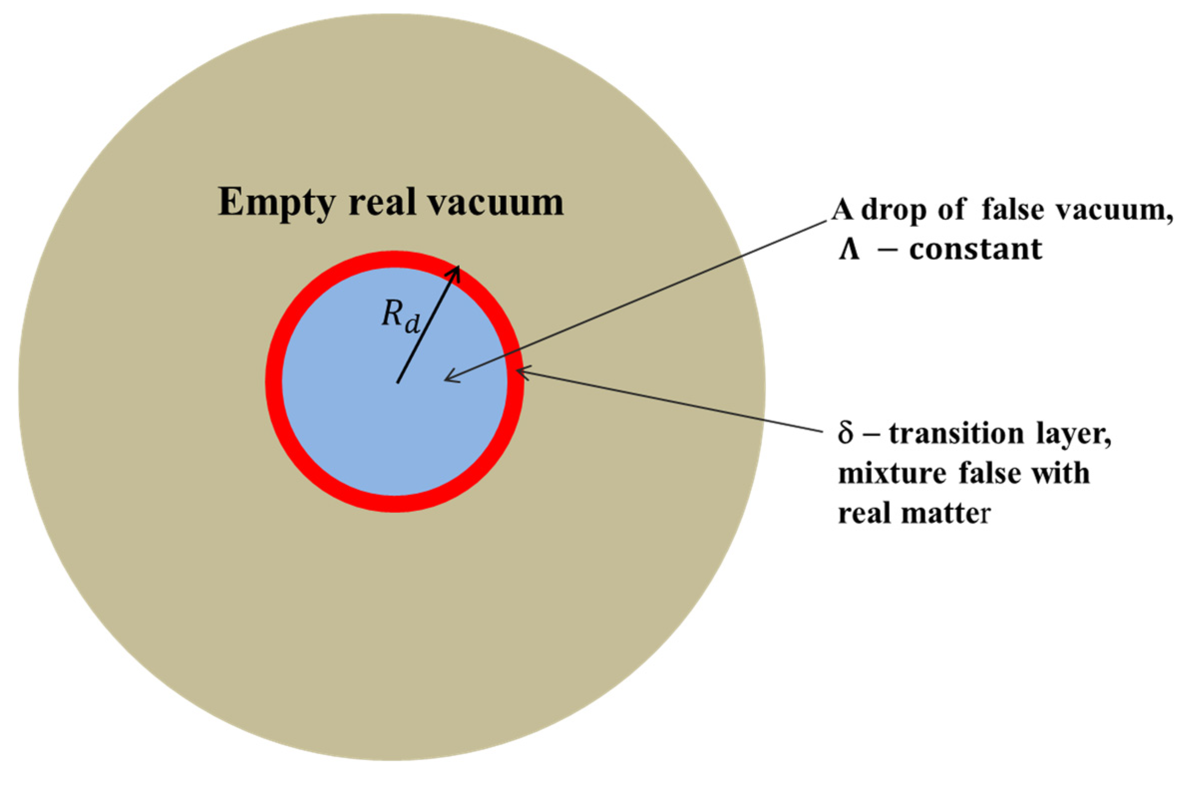
Within the framework of Equations (9) and (10), we consider a singularity-free black hole with a false vacuum drop, shown schematically in Figure 1. We will assume that the radius of the false vacuum region where the cosmological term, lambda, is non-zero is $R_d$ and that the characteristic size of the transition region between the false and physical vacuum is $\delta \ll R_d$. Let us introduce dimensionless variables:

$${\Lambda }_{\ast }={\displaystyle \frac{\Lambda }{{\Lambda }_0}},T_{\ast 0}^0={\displaystyle \frac{8\pi G}{c^4}}{\displaystyle \frac{{\tilde{T}}_0^0}{{\Lambda }_0}},T_{\ast 2}^2={\displaystyle \frac{8\pi G}{c^4}}{\displaystyle \frac{{\tilde{T}}_2^2}{{\Lambda }_0}}x={\displaystyle \frac{r}{r_0}},r_0={\displaystyle \frac{1}{\sqrt{{\Lambda }_0}}},R_{\ast }={\displaystyle \frac{R_d}{r_0}},{\delta }_{\ast }={\displaystyle \frac{\delta }{r_0}},$$

(11)

where ${\Lambda }_0$ is the value of the cosmological constant at the center of the false vacuum bubble, ${\tilde{T}}_0^0$ and ${\tilde{T}}_2^2$ are energy-momentum tensor coefficients associated with gravitating matter at the edge of the false vacuum bubble. All other values ${\tilde{T}}_i^k$ are zero.

The solution of Equations (9) and (10) in dimensionless variables (11) for singularity-free black holes with a drop of false vacuum inside has the following form:

$${\Lambda }_{\ast }=1-{\displaystyle \frac{1}{\sqrt{\pi }}}{\int }_{{\displaystyle \frac{-R_{\ast }}{{\delta }_{\ast }}}}^{{\displaystyle \frac{x-R_{\ast }}{{\delta }_{\ast }}}}{e}^{-y^2}dy,$$

(12)

$$T_{\ast 0}^0={\eta }_{\ast }\left(1-{\displaystyle \frac{1}{\sqrt{\pi }}}{\int }_{{\displaystyle \frac{-R_{\ast }}{{\delta }_{\ast }}}}^{{\displaystyle \frac{x-R_{\ast }}{{\delta }_{\ast }}}}{e}^{-y^2}dy\right){\displaystyle \frac{1}{\sqrt{\pi }}}{\int }_{{\displaystyle \frac{-R_{\ast }}{{\delta }_{\ast }}}}^{{\displaystyle \frac{x-R_{\ast }}{{\delta }_{\ast }}}}{e}^{-y^2}dy,$$

(13)

$$T_{\ast 2}^2=T_{\ast 0}^0+{\displaystyle \frac{x}{2}}\left({\displaystyle \frac{d{T}_{\ast 0}^0}{dx}}-{\displaystyle \frac{d{\Lambda }_{\ast }}{dx}}\right),$$

(14)

$${g_{00}=e}^{-\lambda }=1-{\displaystyle \frac{1}{x}}{\int }_0^x{x}^2\left(T_{\ast 0}^0-{\Lambda }_{\ast }\right)dx,$$

(15)

where $g_{00}$ is the coefficient of metric tensor, ${\eta }_{\ast }={\displaystyle \frac{8\pi G}{c^4}}{\displaystyle \frac{\eta }{{\Lambda }_0}}$ is a dimensionless parameter characterizing the momentum energy tensor.

For case $R_{\ast }\gg {\delta }_{\ast }$, we get an approximation expression for $g_{00}$ as follows:

$${g_{00}=e}^{-\lambda }=\left\{\begin{array}{cc}x<R_{\ast }& 1+{{\displaystyle \frac{1}{3}}x}^2\\ x>R_{\ast }& 1-\left(\alpha R_{\ast }^2{\delta }_{\ast }{\eta }_{\ast }-{\displaystyle \frac{R_{\ast }^3}{3}}\right){\displaystyle \frac{1}{x}}\end{array}\right.,$$

(16)

$$\lambda =\left\{\begin{array}{cc}x<R_{\ast }& -ln\left(1+{{\displaystyle \frac{1}{3}}x}^2\right)\\ x>R_{\ast }& -ln\left(1-\left(\alpha R_{\ast }^2{\delta }_{\ast }{\eta }_{\ast }-{\displaystyle \frac{R_{\ast }^3}{3}}\right){\displaystyle \frac{1}{x}}\right)\end{array}\right..$$

(17)

where

$$\alpha ={\int }_{-\infty }^{\infty }\left(1-{\displaystyle \frac{1}{\sqrt{\pi }}}{\int }_{-\infty }^x{e}^{-y^2}dy\right)\left({\displaystyle \frac{1}{\sqrt{\pi }}}{\int }_{-\infty }^x{e}^{-y^2}dy\right)dx=0.3989.$$

(18)

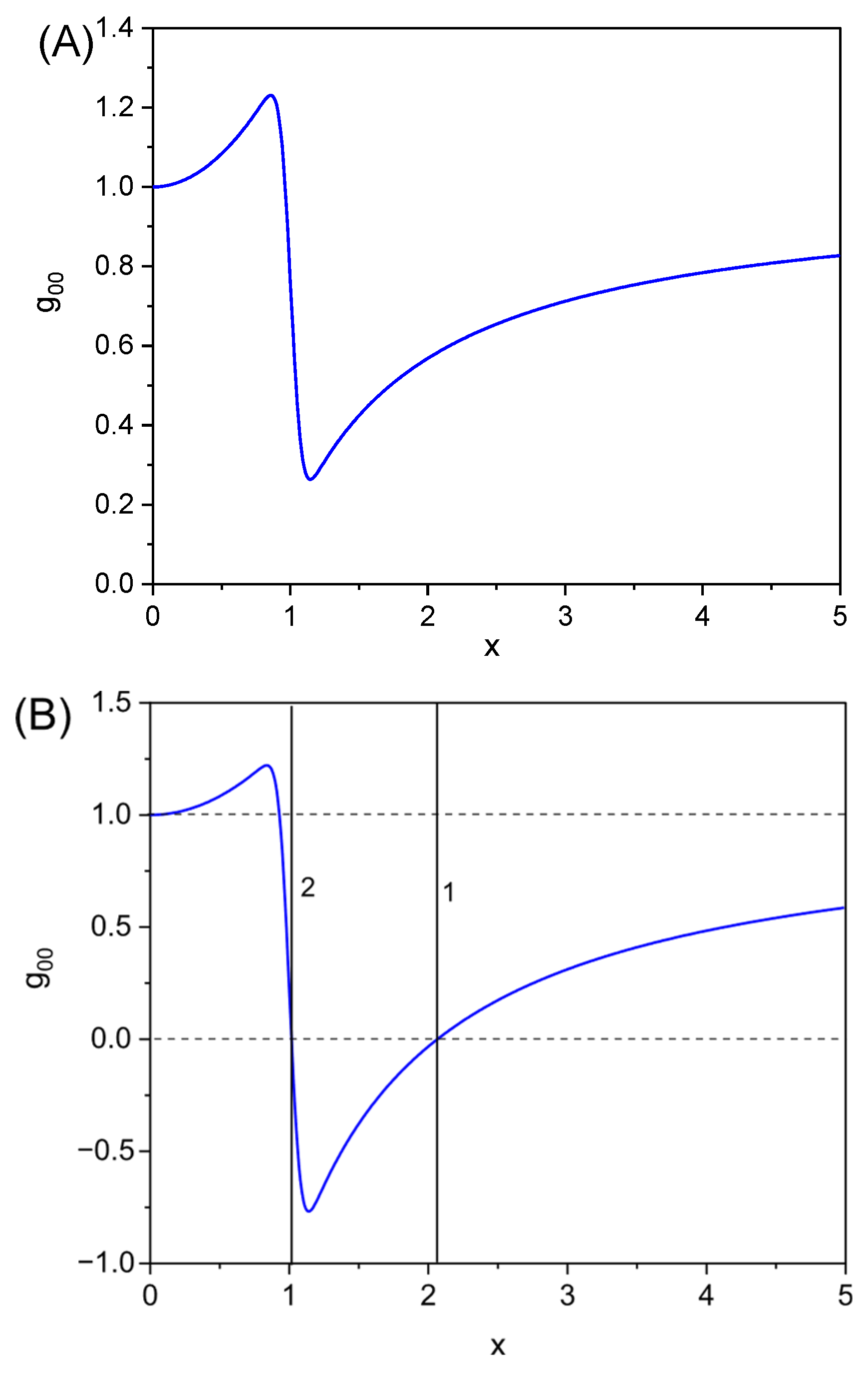
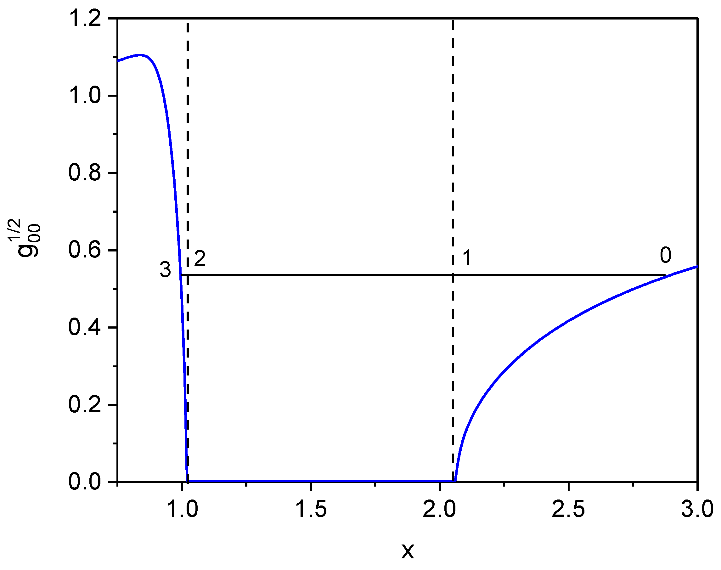
It should be noted that asymptotic (17) for $g_{00}$ coincides with the asymptotic obtained in [16]. Figure 2 shows the dependence of $g_{00}$ on $x$ for ${\eta }_{\ast }=30$, when $g_{00}>0$ for all values of $x$ and for ${\eta }_{\ast }=$60, when there is an interval of $x$ values, where $g_{00}<0$. Vertical lines 1 and 2 correspond to event horizons, where $g_{00}=0.$ Since a singular-free black hole is characterized by the presence of two event horizons, it corresponds to the dependence $g_{00}$ in Figure 2B.

3. Passing Through the Event Horizon of a Classical Black Hole

One problem in modern cosmology is that, according to a frame of reference associated with a remote observer, the time it takes matter to fall through the event horizon is infinite (see [18], for example). Since the universe has a finite lifetime, we can conclude that a black hole can contain only matter that participated in its formation. Thus, from the perspective of a distant observer, matter accreting onto a black hole should accumulate near the event horizon, causing its density to approach infinity. On the other hand, in the frame of reference associated with a body falling onto a black hole, as it approaches the event horizon, the particle velocity tends to the speed of light (and not to zero as in a remote frame of reference) and the time of its penetration beyond the event horizon and further fall into a singularity is finite [19,20]. The contradiction between the finite time of penetration of particles under the event horizon in the frame of reference, associated with the falling body, and infinite in the remote frame, within the framework of the General Theory of Relativity, cannot be resolved.

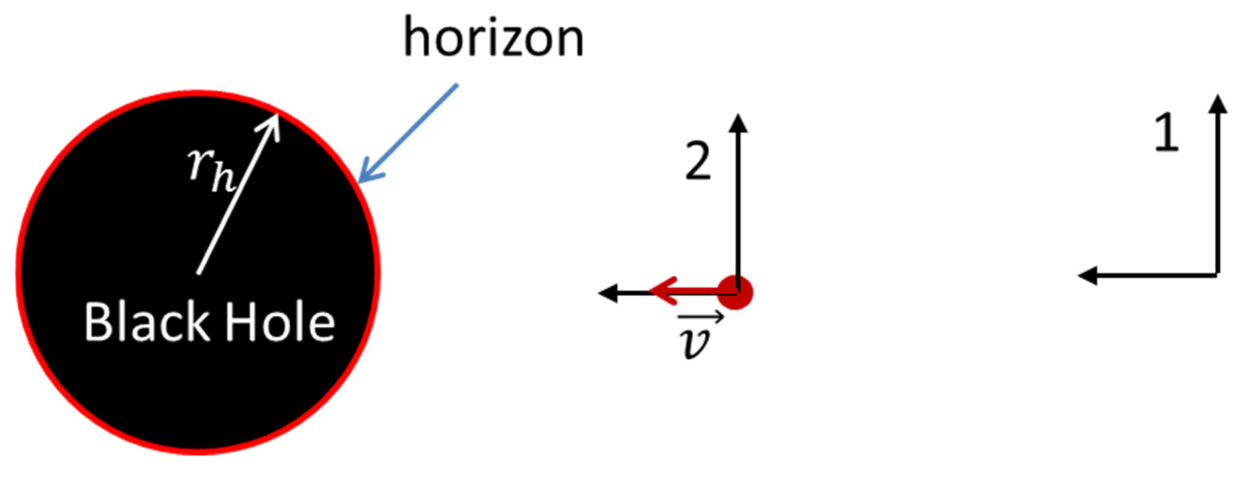
Consider a body falling on a black hole, observed from a remote point where the gravitational field of the black hole can be neglected (Figure 3). If at the initial moment of time the particle is at the point with the coordinate $r_0$ from the center of the black hole and its velocity is equal to zero, then the time of its motion to the point $r$ is determined by the equation [18]:

$$ct={\displaystyle \frac{{\mathcal{E}}_0}{m{c}^2}}{\int }_r^{r_0}{\displaystyle \frac{dr}{g_{00}(r){\left({\left(\frac{{\mathcal{E}}_0^2}{m{c}^2}\right)}^2-g_{00}(r)\right)}^{1/2}}}={\int }_r^{r_0}{\displaystyle \frac{dr}{g_{00}(r){\left(1-\frac{g_{00}\left(r\right)}{g_{00}\left(r_0\right)}\right)}^{1/2}}},$$

(19)

$${\mathcal{E}}_0={\displaystyle \frac{m{c}^2\sqrt{g_{00}}}{\sqrt{1-v_{\tau }^2/c^2}}},$$

(20)

where $v_{\tau }=c{\displaystyle \frac{dl}{d\tau }}=c{\displaystyle \frac{dl}{\sqrt{g_{00}}dt}}=c{\displaystyle \frac{v}{\sqrt{g_{00}}}}$ is the particle velocity measured over time in the frame of reference associated with the location of the particle, ${\mathcal{E}}_0$ in (20) is constant, independent of the position of the particle. In the vicinity of the event horizon $g_{00}\left(r\right)=\left(1-{\displaystyle \frac{r_h}{r}}\right)$, where $r_h={\displaystyle \frac{2GM}{c^2}}$—is the radius of the event horizon, and at the particle stopping point $v_{\tau }=v=0$, $g_{00}\left(r_0\right)\approx 1-{\displaystyle \frac{r_g}{r_0}}$. Accordingly:

$$ct\approx {\left(1-{\displaystyle \frac{r_h}{r_0}}\right)}^{1/2}{\int }_r^{r_0}{\displaystyle \frac{dr}{\left(1-\frac{r_h}{r}\right){\left(\frac{r_h}{r}-\frac{r_h}{r_0}\right)}^{1/2}}}.$$

(21)

From (21) it follows that for $r$ close enough to $r_h$, $t$ changes as:

$$t={\displaystyle \frac{r_h}{c}}ln\left({\displaystyle \frac{r_0-r_h}{r-r_h}}\right),$$

(22)

and the velocity changes as:

$$v={\displaystyle \frac{c}{r_h}}\left(r-r_h\right).$$

(23)

From (22) and (23) it follows that in a remote frame of reference the velocity of the body tends to zero when approaching the event horizon, and the time of approach tends to infinity.

Now let us make some general comments. Firstly, we cannot connect the frame of reference with an electron or any other elementary particle, since its velocity in it is equal to zero, and this means that the position of the particle is uncertain due to the Heisenberg uncertainty principle $\Delta x~\mathsf{ħ}/\Delta \mathrm{p}$. Secondly, as the particle approaches the event horizon, its velocity in the remote reference frame tends to zero and the wave properties begin to play a role.

Consider, for simplicity, a single particle approaching the horizon. According to the uncertainty principle:

$$mv\left|r-r_h\right|={\displaystyle \frac{mc}{r_h}}{\left(r-r_h\right)}^2={\displaystyle \frac{cm{\left(r_0-r_h\right)}^2}{r_h}}{e}^{-2ct/r_h}\approx \mathsf{ħ},$$

(24)

where $\mathsf{ħ}$ is the Planck constant.

From (24) it follows that when the distance of the particle to the event horizon becomes of the order:

$$\delta r=\left(r-r_h\right)~\sqrt{{\displaystyle \frac{r_h\mathsf{ħ}}{mc}}}=\sqrt{r_h{\lambda }_{compt}},$$

(25)

and its velocity, accordingly, decreases to the value:

$$v~c\sqrt{{\displaystyle \frac{{\lambda }_{compt}}{r_h}}},$$

(26)

The particle is equally probable to be both behind the horizon and below the horizon. In (25) and (26) ${\lambda }_{compt}={\displaystyle \frac{\hslash }{cm}}$ is the Compton particle length. Thus, in a remote frame of reference, mass particles must approach the event horizon at a distance of the order of $\delta r~\sqrt{r_h{\lambda }_{compt}}$ to be captured by a black hole.

Substituting (25) into (22), we find an estimate for the time of passage of a particle through the horizon:

$$t\approx {\displaystyle \frac{r_h}{c}}ln\left({\displaystyle \frac{r_0}{r_h}}\right)+{\displaystyle \frac{r_h}{2c}}ln\left({\displaystyle \frac{r_h}{{\lambda }_{compt}}}\right)=t_{r_0}+t_h.$$

(27)

In (27), $t_{r_0}={\displaystyle \frac{r_h}{c}}ln\left({\displaystyle \frac{r_0}{r_h}}\right)$ is the times related to the initial position of the particle, and $t_h={\displaystyle \frac{r_h}{2c}}ln\left({\displaystyle \frac{r_h}{{\lambda }_{compt}}}\right)$ is not. For an electron ${\lambda }_{compt,e}={4\times 10}^{-13}$ m and for a proton ${\lambda }_{compt,p}={2\times 10}^{-16}$ m. Accordingly, for a black hole with an event horizon radius $r_h=3\times {10}^3$ m, which corresponds to the mass of a black hole equal to the mass of the sun, for a proton $t_h=2.1\times {10}^{-4}$ s, $v=0.08$ m/s, $\delta r=7.7\times {10}^{-7}$ m, and for an electron $t_h=1.8{\times 10}^{-4}$ s and $v=3.5$ m/s, $\delta r=3.4\times {10}^{-5}$ m.

Thus, in a distant frame of reference, mass particles must approach the event horizon at a distance of the order of $\delta r~\sqrt{r_h{\lambda }_{compt}}$ to be captured by a black hole.

Let us compare the mechanism described above, of a particle captured by a black hole due to quantum mechanical “jitter” of the event horizon [3]. In accordance with [3], the fluctuation of the event horizon position is $\delta r_h~{\displaystyle \frac{l_p^2}{r_h}}$, where $l_p={\left(\mathsf{ħ}G/c^3\right)}^{1/2}\approx 1.6\times {10}^{-35}$ m is the Planck length. For $r_h=3\times {10}^3$ m we get $\delta r_h~8.6\times {10}^{-74}$ m. That is, a particle must approach the event horizon at a distance of $8.6\times {10}^{-74}$ m to be captured by a black hole. This distance is 59 orders of magnitude less than the classical radius of an electron and 58 orders of magnitude less than the radius of a proton. However, in accordance with (22), the time of movement of a particle until it crosses the horizon differs only by an order of magnitude from estimate (27) for an electron and a proton:

$$t~{\displaystyle \frac{r_h}{c}}ln\left({\displaystyle \frac{r_0}{\delta r}}\right)={\displaystyle \frac{r_h}{c}}ln\left({\displaystyle \frac{r_0}{r_h}}\right)+{\displaystyle \frac{r_h}{c}}ln\left({\displaystyle \frac{r_h}{\delta r_h}}\right)=t_{r_0}+t_{\delta r_h}.$$

(28)

For $r_h=3\times {10}^3$ m, $t_{\delta r_h}=1.7\times {10}^{-2}$ s.

The use of quantum mechanical properties of particles for their passage through the event horizon was first considered by Hawking [21]. Note, that it is shown in [22] that atoms falling into a black hole emit radiation which looks to a distant observer much like Hawking radiation, but this radiation is different.

Since the Compton length of a particle depends on its mass, let us show that even before the body approaches the horizon at the distance of the Compton length of an electron, it disintegrates into elementary particles.

It is known (see, for example [23,24,25]) that when any bodies approach a black hole, tidal forces $f_g~1/(r-r_h)$, act on them which leads to the destruction of any objects, down to atoms and molecules, approaching sufficiently close to the black hole. Let us estimate the distance to the event horizon at which ionization of atoms begins and compare with the distance at which the capture of electrons and protons by a black hole occurs.

In accordance with [18], the force acting on a particle in a constant gravitational field has the form:

$$f_g=-{\displaystyle \frac{m{c}^2}{\sqrt{1-v^2/c^2}}}{\displaystyle \frac{1}{2g_{00}}}{\displaystyle \frac{\partial g_{00}}{\partial r}}\approx -{\displaystyle \frac{m{c}^2}{2\left({r-r}_h\right)}}.$$

(29)

In (29), we took into account that in the frame of reference of a remote observer, the particle velocity near the event horizon is close to zero. Substituting in (19) the value ${r-r}_g$ from (25) we get

$$f_g\approx -{\displaystyle \frac{m{c}^2}{2\sqrt{r_g{\lambda }_{compt}}}}.$$

(30)

The force acting on an electron near the horizon of a black hole with $r_g=1$ m is $f_{g,e}=3.31\times {10}^{12}$ eV/m, and on a proton, respectively, $f_{g,p}=3.3\times {10}^{16}$ eV/m. Let us estimate the tidal forces acting on particles near the event horizon. Differentiating (19) with respect to $r$, we obtain:

$${\displaystyle \frac{\partial f_g}{\partial r}}\approx {\displaystyle \frac{m{c}^2}{2{\left({r-r}_g\right)}^2}}.$$

(31)

Accordingly, the work $A_g$, performed by the gravitational field to separate charges in an atom can be estimated as $A_g={\displaystyle \frac{\partial f_g}{\partial r}}{a}^2$, where $a$ is the size of the electron’s orbit. Hence,

$$A_g\approx {\displaystyle \frac{m{c}^2}{2{\left({r-r}_g\right)}^2}}{a}^2~I.$$

(32)

where $I$ is the ionization potential of the atom. From (32) we find the distance to the event horizon at which the atom is ionized:

$$\left({r-r}_g\right)~a\sqrt{{\displaystyle \frac{m{c}^2}{2I}}}.$$

(33)

Substituting in (29) $a~10^{-10}$ m, $I=13$ eV, $m{c}^2=500$ keV, we obtain for the hydrogen atom, ${r-r}_g~{10}^{-8}\mathrm{m}\gg {\lambda }_{compt,e}$. In the case of molecules, it is obvious that molecular bonds will break down long before ionization.

Let us make a similar estimate for the atomic nucleus. Since the maximum binding energy of a nucleon in the nucleus does not exceed 9 MeV, the self-energy of a neutron is 930 MeV, then substituting in (29) $I=9$ MeV, ${Mc}^2=930$ Mev,$a~2\times {10}^{-15}$ m, we get $\left({r-r}_g\right)~{10}^{-14}\gg {\lambda }_{compt,p}$. In other words, the nuclei will decay into individual nucleons before the nucleons, due to quantum properties, cross the event horizon.

4. Particle Motion in the Gravitational Field of a Non-Singular Black Hole

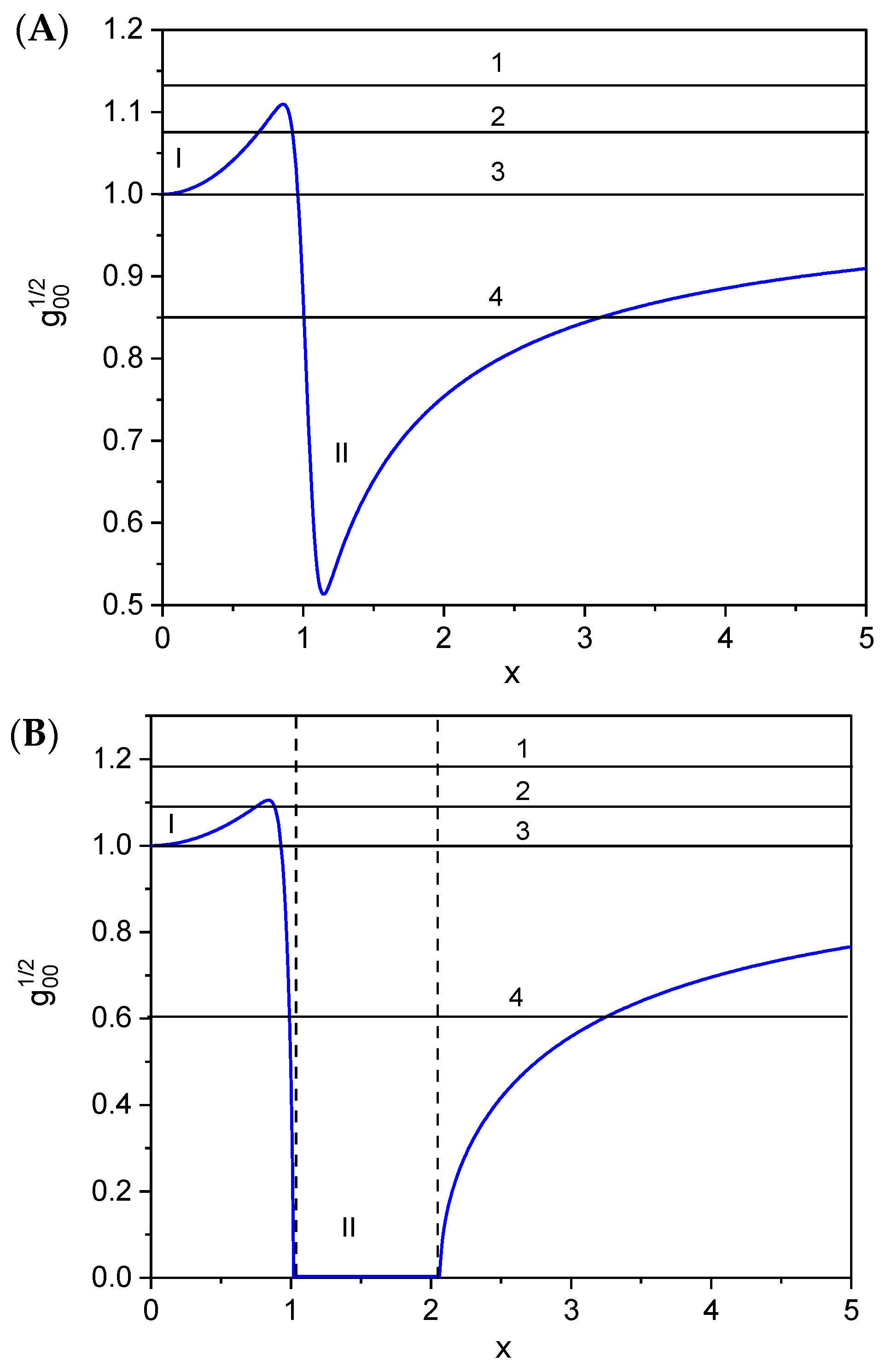
Figure 4 shows the dependence $\sqrt{g_{00}\left(x\right)}$ for positive values of $g_{00}$. Let us consider Figure 4A. Line 1 corresponds to a transit particle, its energy at infinity is finite $E_{\infty }=m{c}^2/\sqrt{1-v^2/c^2}>m{c}^2$; line 2 corresponds to the particle reflected by the barrier I, its energy at infinity $E_{\infty }$ also greater than $m{c}^2$; line 3 corresponds to a particle with zero kinetic energy at infinity, $E_{\infty }=m{c}^2$; line 4 corresponds to the particle trapped in well II.

Now let us turn to the non-singular black hole, which corresponds to Figure 4B. If there was no region in which $g_{00}<0$, then all our reasoning related to particles 1, 2, 3, 4 in Figure 4A could be attributed to particles in Figure 4B. The question is: is the time of movement of particles finite through the region of negative values $g_{00}$ in the reference frame of the distant observer (where $g_{00}>0$) or not?

The time of passage of a particle through the event horizon for a singular black hole $t_h={\displaystyle \frac{r_h}{2c}}ln\left({\displaystyle \frac{r_h}{{\lambda }_{compt}}}\right)$, obtained above in Part 3, is also valid for non-singular black holes. Let us find the time spent by the particle in the region of negative values of $g_{00}$.

Figure 5 shows the motion of a particle along the trajectory 0 → 1 → 2 → 3.

Points $r_0$ and $r_3$ correspond to stop points, points $r_1$ and $r_2$ correspond to the positions of the event horizons. Obviously, the time of motion of a particle $t_{01}$ from a point with a coordinate $r_0$ to a point with a coordinate $r_1+\delta r_1$, $\delta r_1=\sqrt{{\lambda }_{compt}{r}_1}$ and the time of motion of a particle $t_{23}$ from point with coordinate $r_2-\delta r_2$, $\delta r_2=\sqrt{{\lambda }_{compt}{r}_2}$ to a point $r_3$ is finite, since in these regions $g_{00}$ is finite and is greater than zero (9), and at the stopping points $1-{\displaystyle \frac{g_{00}\left(r\right)}{g_{00}\left(r_0\right)}}~{\left|\delta r_s\right|}^{1/2}$, where $\delta r_s$ is the distance to the stopping points. The time of particle motion in the region limited by the event horizons is also finite, since $g_{00}\left(r\right)$ in the interval $\left(r_1-\delta r_1,r_2+\delta r_2\right)$ is limited, and $1<1-{\displaystyle \frac{g_{00}\left(r\right)}{g_{00}\left(r_0\right)}}<1-{\displaystyle \frac{g_{00}\left(r_{\ast }\right)}{g_{00}\left(r_0\right)}}$, $r_{\ast }$ is the coordinate of the minimum of the function $g_{00}\left(r\right)$.

We see that the dynamics of particles falling on a singular-free hole does not actually differ from the dynamics of particles falling on a false vacuum drop with a gravitating shell without horizons.

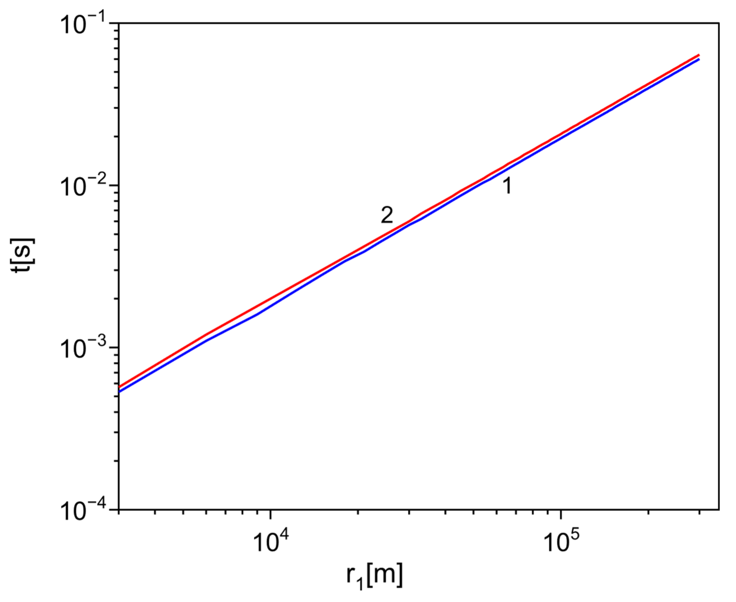
Figure 6 shows the dependence of the time of particle motion on the radius of the event horizon from point 0 to point 3 and back, $\left({\displaystyle \frac{{\mathcal{E}}_0-m{c}^2}{m{c}^2}}\right)\ll 1$, $g_{00}\left(r_0\right)\ll 1$ (Figure 5).

As can be expected, at fixed values of ${\eta }_{\ast }$, $R_{\ast }$, ${\delta }_{\ast }$, the time of motion of particles on a nonsingular black hole grows linearly with its size.

5. Accretion on Non-Singular Black Holes and Radiation

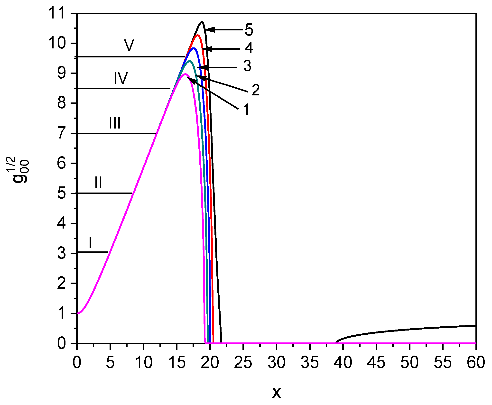
Before we move on to the issue of particle emission from a singular-free black hole, we make two remarks. The height of the energy barrier I in Figure 4 depends on the distribution of the false vacuum and gravitating matter at the boundary. Figure 7 shows the dependence of the height of the energy well barrier I on ${\delta }_{\ast }$ at ${\eta }_{\ast }=17$, $R_{\ast }=20$, where ${\delta }_{\ast }$ is the thickness of the transition layer. As expected, the barrier height decreases with increasing ${\delta }_{\ast }$. In addition, the accretion of matter onto a drop of false vacuum with a gravitating shell leads to a decrease in the height of the barrier of well I due to the filling of well II with the gravitating substance.

Thus, if well is filled with matter, then accretion onto a false vacuum drop with a gravitating shell should lead to the outflow of matter from the well.

Since at the point of reflection $x$ in the particle velocity is zero, $v\left(x_{in}\right)=0$, then:

$${\mathcal{E}}_0=m{c}^2\sqrt{g_{00}\left(x_{in}\right)},p={\displaystyle \frac{mv}{\sqrt{1-v^2/c^2}}}=mc{\displaystyle \frac{\sqrt{g_{00}\left(x_{in}\right)-g_{00}}}{\sqrt{g_{00}}}}.$$

(34)

Accordingly, for the levels below the edge of the energy well:

$$\xi ={\displaystyle \frac{2}{\mathsf{ħ}}}{\int }_0^{r_{in}}pdr={\displaystyle \frac{2r_0}{\mathsf{ħ}}}{\int }_0^{x_{in}}pdx={\displaystyle \frac{{2r}_{0}mc}{\mathsf{ħ}}}{\int }_0^{x_{in}}{\displaystyle \frac{\sqrt{x_{in}^2-x^2}}{\sqrt{3+x^2}}}dx={\displaystyle \frac{{2r}_0}{{\lambda }_{compt}}}{x}_{in}^2{\int }_0^1{\displaystyle \frac{\sqrt{1-y^2}}{\sqrt{3+x_{in}^2{y}^2}}}dy.$$

(35)

From Bohr’s quantization condition $\xi$ should have integer values. Therefore, if $\xi <1$, then there are no possible levels in the well. Assuming that $r_0$ is of the order of the Planck dimension ${~10}^{-35}$ m, then for electrons ${\displaystyle \frac{{2r}_0}{{\lambda }_{compt}}}=5\times {10}^{-23}$, for protons ${\displaystyle \frac{{2r}_0}{{\lambda }_{compt}}}={10}^{-19}$ and, accordingly, $x_{in}\gg 1$. In this case, we obtain an estimate for ξ:

$$\xi \approx {\displaystyle \frac{{2r}_0}{{\lambda }_{compt}}}{x}_{in}\ln \left(x_{in}\right).$$

(36)

In accordance with (28) and the Bohr quantization conditions for the n-th level:

$$x_{in,n}\approx {\displaystyle \frac{{\lambda }_{compt}}{{2r}_{0}ln\left({\lambda }_{compt}/{2r}_0\right)}}n.$$

(37)

In this case, up to a logarithm accuracy, we obtain

$${\mathcal{E}}_n=m{c}^2\sqrt{g_{00}\left(x_{in,n}\right)}\approx m{c}^2{x}_{in,n}\approx {\displaystyle \frac{1}{2\sqrt{3}}}{\displaystyle \frac{\hslash c}{r_0}}n{\displaystyle \frac{1}{ln\left(\frac{{\lambda }_{compt}}{{2r}_0}\right)}}n\approx 2\times {10}^{8}n[\mathrm{J}\mathrm{o}\mathrm{u}\mathrm{l}\mathrm{e}\mathrm{s}].$$

(38)

Figure 7 shows the dependence of $\sqrt{g_{00}}$ on $x$ for various values of ${\delta }_{\ast }/R_{\ast }$. Energy levels are indicated by Roman numerals. At ${\delta }_{\ast }/R_{\ast }>0.075$, particles at level V are emitted and leave the singular-less black hole. For $x>2$, $\sqrt{g_{00}}$ grows linearly up to the edge of the barrier with increasing $x$.

Note that, although the energies ${\mathcal{E}}_n$ are independent of the particle masses, the reflection points $x_{in,n}$ are not. This is a fundamental situation, since with a decrease in the depth of the well I, light particles will leave it first, since the values $x_{in,n}$for them are greater than for heavy ones. If the trapped particles in well I are electrons and protons, then a singular-less black hole is a “quasi-atom” since the levels for electrons in the $\sqrt{g_{00}\left(x\right)}$ graph lie much higher than those for protons. The question of the charge of a singular-free black hole, the interaction of trapped particles with each other, and the effect on the values of the metric coefficients are beyond the scope of this work and require separate consideration.

Note that one way to prove the existence of nonsingular black holes would be to observe an “echo” in radiation bursts associated with falling particles in the radiation bursts associated with particles that intersect the event horizon. The delay time between the flash and the echo reveals how long it takes particles to travel from the event horizon to the false vacuum region in the core of a nonsingular black hole. However, this topic is beyond the scope of our article and requires further consideration.

6. Conclusions

It has been shown that

1.

When particles in a frame of reference associated with a distant observer approach the event horizon, their wave properties begin to dominate. This makes it possible to estimate the time it takes particles to pass through the event horizon when observed in a distant frame of reference.

2.

In a frame of reference associated with a distant observer, the oscillatory motion of a particle in a nonsingular black hole is always limited.

3.

As matter is accreted onto a nonsingular black hole, the value of the barrier holding particles near its center decreases. This leads to the emission of matter from the black hole to the outside. A distant observer can interpret this radiation process as a white hole.